Vertical Shear, Diapycnal Shear and the Gradient Richardson Number

Preprint

Article

Vertical Shear, Diapycnal Shear and the Gradient Richardson Number

Altmetrics

Downloads

Views

Comments

A peer-reviewed article of this preprint also exists.

Josep L. Pelegrí^*

Mariona Claret,Pablo Sangrà

Josep L. Pelegrí^*

Mariona Claret,Pablo Sangrà

This version is not peer-reviewed

Submitted:

17 July 2024

Posted:

17 July 2024

You are already at the latest version

Alerts

Abstract

In vertical coordinates, (x,y,z), the gradient Richardson number Ri=N^2⁄S^2 is the square of the ratio between buoyancy frequency N and vertical-shear amplitude S, where N^2=-(g⁄ρ) ∂ρ⁄∂z and S^2=(∂u⁄∂z)^2+ (∂v⁄∂z)^2, with ρ potential density, (u,v) the horizontal velocity components and g gravity acceleration, so that a decrease in stratification brings a decrease in dynamic stability and vice versa. In the isopycnic coordinate system, (x,y,ρ), however, Ri=M^2⁄〖S_ρ〗^2 , is the ratio between 〖M^2≡N〗^(-2) and the squared diapycnal shear 〖S_ρ〗^2=(ρ⁄g)^2 [(∂u⁄∂ρ)^2+ (∂v⁄∂ρ)^2 ], so a decrease in stratification leads to an increase in dynamic stability and vice versa. The apparently different role of stratification arises because S and S_ρ are related through the stratification itself, S_ρ=S⁄N^2 or, equivalently, τ=〖t_o〗^2⁄t_d , which is interpreted as a natural oscillation time τ≡S_ρ that equals the buoyancy or oscillation time t_o=N^(-1) normalized by the ratio t_o⁄t_d , where the deformation time is t_d=S^(-1). Here we follow simple arguments and use field data from three different situations (island shelf-break, Gulf Stream and Mediterranean outflow) to endorse the usefulness of the isopycnal approach. In particular, we define the reduced squared vertical σ^2= S^2-N^2 and reduced squared diapycnal shear 〖σ_ρ〗^2= 〖S_ρ〗^2-M^2, which are positive for unstable conditions and negative for stable conditions. It turns out that Ri and σ^2 remain highly variable for all stratification conditions; in contrast, the mean 〖σ_ρ〗^2 values display a univocal tendency, its magnitude decreasing with stratification. We propose 〖σ_ρ〗^2 and 〖S_ρ〗^2 to be good indexes for the occurrence of effective mixing under high stratification conditions.

Keywords:

Subject: Environmental and Earth Sciences - Oceanography

1. Introduction

The analysis of small flow perturbations, for the case of uniformly stratified and sheared flow, goes back to Geoffrey Taylor’s 1915 essay for the Adams Prize (Taylor, 1931a), later followed by many other researchers, specially Miles (1961), Howard (1961), and Abarbanel et al. (1984, 1986). Other authors employed energetic arguments to assess under which conditions the energy of fluctuations will increase, among them Richardson (1920), Taylor (1931b), and Miles (1986) (for a brief historical review see Van Gastel and Pelegrí, 2004). The conclusion from these works is that the growth of flow perturbations may be expressed in terms of the (gradient) Richardson number, Ri, with perturbations remaining stable when the Richardson number is above some critical value

{R i}_{c}

(supercritical,

R i > {R i}_{c}

) but becoming unstable when it goes below (subcritical,

R i < {R i}_{c}

). Abarbanel et al. (1986) showed that nonlinear stability analysis of three-dimensional stratified shear flow leads to a critical value of one, in agreement with energy arguments (Miles, 1986). Despite so, there are yet some theoretical and observational uncertainties on the actual Ri threshold value for the development of turbulence (Grachev et al., 2013; Roget et al., 2023).

The most common representation for the Richardson number comes in the vertical Cartesian

(x, y, z)

coordinate system,

R i = \frac{- (\frac{g}{ρ}) \frac{\partial ρ}{\partial z}}{{(\frac{\partial u}{\partial z})}^{2} + {(\frac{\partial v}{\partial z})}^{2}} = \frac{N^{2}}{S^{2}}

(1)

with ρ the potential density and

(u, v)

the velocity horizontal components in the horizontal

(x, y)

directions. Both the oscillation or buoyancy frequency

N = {[- (g / ρ) \partial ρ / \partial z]}^{1 / 2}

and vertical shear

S = {[{(\partial u / \partial z)}^{2} + {(\partial v / \partial z)}^{2}]}^{1 / 2}

have frequency units.

Multiplying and dividing equation (1) by

{[(ρ / g) \partial z / \partial ρ]}^{2}

immediately leads to the gradient Richardson number in the

(x, y, ρ)

isopycnic Cartesian coordinate system

R i = \frac{- (\frac{ρ}{g}) \frac{\partial z}{\partial ρ}}{{(\frac{\partial u}{\partial ρ})}^{2} + {(\frac{\partial v}{\partial ρ})}^{2}} = \frac{M^{2}}{{S_{ρ}}^{2}}

(2)

where

{M \equiv N}^{- 1} = {[- (ρ / g) \partial z / \partial ρ]}^{1 / 2}

is the buoyancy or oscillation period, and

S_{ρ} = (ρ / g) {[{(\partial u / \partial ρ)}^{2} + {(\partial v / \partial ρ)}^{2}]}^{1 / 2}

is the diapycnal shear, both with units of time. We introduce the “diapycnal shear” terminology to emphasize that the derivatives are with respect to density, when multiplied by

ρ / g

the result has time units.

A paradox arises: from the vertical perspective Ri is directly proportional to stratification while from the isopycnic perspective Ri is inversely proportional to stratification (Pelegrí and Csanady, 1994; Pelegrí and Sangrà, 1998; Pelegrí et al., 1998). The answer lies on the fact that the vertical and diapycnal shear are related through stratification,

S = N^{2} S_{ρ}

. For constant vertical shear an increase in stratification enhances dynamic stability; for constant diapycnal shear, however, this same increase actually reduces dynamic stability as it implies a quadratic increase in vertical shear. We are undoubtedly most used to the vertical perspective so perhaps we are missing some lessons that may be learned from the isopicnic view. In this work we will pursue such an isopycnic inspection, by means of both simple conceptual arguments and through the analysis of real data for different dynamic situations.

In next section we explore some relevant differences between the vertical and isopycnic perspectives, and introduce the concepts of natural oscillation time, reduced squared vertical shear and reduced squared diapycnal shear. We present the non-dimensional variables in section 3, examining the inter-dependence between background stratification, vertical shear and diapycnal shear. The three data sets used in our study are briefly described in section 4, and in section 5 we look at these data in two different ways: first as cloud points plotted in terms of two variables (among background stratification, vertical shear and diapycnal shear) and next examining the dependence of both the reduced squared vertical shear and the reduced squared diapycnal shear in terms of the background stratification. Finally, in section 6 we summarize the main conclusions.

2. Isopycnic versus Vertical Perspectives

2.1. Basic Considerations

In vertical coordinates, the critical Richardson number criterion is commonly interpreted as if sufficiently high stratification (high N), leads to stable conditions (

R i > 1

), provided the vertical shear remains moderate, while low stratification is prone to unstable conditions (

R i < 1

) (equation 1). In a layered ocean, with near-constant density layers (treads) bounded by steps of rapid density changes (risers), this vertical-coordinate perspective would usually associate the risers to stable regions and the treads to unstable layers. This is true for a static ocean, but dynamic stability depends on the vertical shear. A tread will have most properties well mixed so that both N and S tend to zero; weak vertical shear will lead to instabilities but these will only redistribute near-homogeneous water. In a riser, on the other hand, N is large and instabilities can effectively redistribute density (and other water properties) but these will only develop for large enough vertical shear S.

Equation (2), on the other hand, suggests that a highly stratified region (a riser,

M = N^{- 1} \to 0

) may be prone to mixing as long as the diapycnal shear

S_{ρ}

, which depends on the velocity of water parcels in adjacent layers, remains finite. Consider, for example, a frontogenetic situation where the isopycnals get steeper with time but vertical stratification does not change. The thermal wind equation in isopycnic coordinates,

ρ f \partial v / \partial ρ = g \partial z / \partial x

, where f is the Coriolis parameter, tells us that in this case

S_{ρ}

will increase, i.e. there is no need for a decrease in stratification for the flow to become dynamically unstable.

The above simple arguments suggest that diapycnal shear may be a convenient variable to analyse whether sheared oceanic flows are prone to mix. As an illustrative example, consider the two-layer flow between parallel planes such as that set up in the laboratory to simulate interfacial Kelvin-Helmholtz instabilities, e.g. Cisneros-Aguirre et al. (2001) and references therein. The upper and lower layers respectively have densities

ρ = ρ_{0} (1 - ∆)

and

ρ = ρ_{0} (1 + ∆)

, and the corresponding velocities are

u = ∆ g t s i n θ

and

- ∆ g t s i n θ

, where θ is the tilting of the table in the experimental setup. The vertical shear between both layers is not uniquely defined but, in contrast, the isopycnic derivative of the horizontal velocity is easily calculated from

ρ = ρ_{0} (1 - u / (g t s i n θ))

, as

\partial u / \partial ρ = - (g t s i n θ) / ρ_{0}

; notice this derivative is equal to the finite-difference fraction,

δ u / δ ρ = (2 g t ∆ s i n θ) / (2 ρ_{0} ∆) = (g t s i n θ) / ρ_{0}

. The resulting expression for the diapycnal shear is simply

S_{ρ} = t s i n θ

, with time units, implying that instabilities will develop independently of stratification if sufficient time is allowed.

2.2. Characteristic Times

As mentioned in the Introduction, the Richardson number criterion arises from either flow stability or energy arguments. A complementary interpretation comes in terms of characteristic times associated to the inverse of the buoyancy frequency and the vertical shear, as well as to the diapycnal shear itself. The inverse of the buoyancy frequency is the time characteristic for the vertical oscillation of a water parcel in a stratified media, hereafter the buoyancy or oscillation time,

t_{o} = N^{- 1}

. The inverse of the vertical shear gives a characteristic time for the horizontal deformation of a water parcel (or temporal rate of strain), henceforth the vertical deformation time,

t_{d} = S^{- 1}

The diapycnal shear is proportional to the derivative of the horizontal velocity with respect to density, e.g.

\partial u / \partial ρ

; when we multiply this derivative by

ρ / g

we get the diapycnal shear with has units of time, so we set

τ \equiv S_{ρ}

to simply remind us of its time units. As stated before, the vertical and diapycnal shears are related through the stratification,

S_{ρ} = S / N^{2}

or, equivalently, the diapycnal shear is related to the buoyancy and deformation times as

τ = {t_{o}}^{2} / t_{d}

. The diapycnal shear is independent of stratification, as it does not depend on how close the isopycnals are to each other, so we interpret τ as the natural oscillation time of the system, equal to the vertical oscillation time

t_{0}

normalized by the ratio

(t_{0} / t_{d})

Equations (1, 2) may hence be written in terms of these characteristic times as

R i = \frac{N^{2}}{S^{2}} = {(\frac{t_{d}}{t_{o}})}^{2}

(3)

R i = \frac{1}{{N^{2} S_{ρ}}^{2}} = {(\frac{t_{0}}{τ})}^{2}

(4)

or alternatively as

R i = \frac{1}{S S_{ρ}} = \frac{t_{d}}{τ}

(5)

We may now see that equations (3) and (5) are not really that different. According to equation (3), the Richardson number is subcritical (less than one) when

t_{0} > t_{d}

, i.e. when the vertical excursion the water parcel takes long enough for it to become greatly distorted. Similarly, equation (5) tells us that subcritical conditions require a short deformation time

t_{d}

as compared with the natural deformation time τ. The main difference lies on the linear and quadratic dependences: in vertical coordinates the dependence is quadratic

{(t_{d} / t_{0})}^{2}

while in isopycnal coordinates it is linear

(t_{d} / τ)

. Equations (3) and (5) further tell us that the instability condition implies

t_{d} < t_{0} < τ

2.3. Reduced Squared Shears

Kunze et al. (1990) and Sun et al. (1998) introduced the reduced vertical shear,

S - 2 N

, as a complementary way to understand the relevance of subcritical Ri conditions for mixing. The squared root of

R i = N^{2} / S^{2} < 1 / 4

leads to the condition

(S + 2 N) (S - 2 N) > 0

or, alternatively, to the condition of reduced shear greater than zero,

S - 2 N > 0

. A formal advantage of the reduced shear is that it is approximately proportional to the growth rate of Kelvin-Helmholtz instabilities (Hazel, 1972). A practical advantage is that reduced shear helps assess when effective mixing occurs. As mentioned above, growing instabilities are effective blenders in well stratified conditions; in poorly stratified conditions, however, they can only redistribute water which is already well mixed. The Richardson number Ri is not capable of distinguishing cases of low stratification and low shear from those of high stratification and high shear but the reduced shear does, i.e., for two different situations (high and low stratification) with equal Ri subcritical values, it turns that

S - 2 N

is larger (less negative) for the well-stratified condition (Kunze et al., 1990; Sun et al., 1998).

Let us pursue these ideas and define a reduced squared vertical shear

σ^{2}

and a reduced squared diapycnal shear

{σ_{ρ}}^{2}

, which are positive for unstable conditions and negative for stable conditions:

σ^{2} = S^{2} - N^{2} = S^{2} (1 - R i) = N^{2} (1 - R i) / R i

(6)

{σ_{ρ}}^{2} = {S_{ρ}}^{2} - M^{2} = {S_{ρ}}^{2} (1 - R i) = (1 / N^{2}) (1 - R i) / R i

(7)

For a critical gradient Richardson value of one, the condition for instability (

R i = N^{2} / S^{2} = M^{2} / {S_{ρ}}^{2} < 1

) complies both

σ^{2} > 0

and

{σ_{ρ}}^{2} > 0

. The first equality of equations (6) and (7) shows how, for any constant Ri value,

{σ_{ρ}}^{2}

increases with stratification up to a maximum value of

{S_{ρ}}^{2}

; this is not so for

σ^{2}

which displays a monotonic quadratic decrease with stratification, from

S^{2}

to increasingly negative values.

The second equality in equations (6) and (7) illustrates how, for constant Ri values, the reduced squared shears change with either stratification or vertical/diapycnal shear. Both reduced squared shears are equal to the corresponding squared shear but with a

(1 - R i)

reduction factor, i.e. the reduced squared shears increase with decreasing

R i

up to a maximum value equal to the squared shear, with

σ^{2}

approaching

S^{2}

and

{σ_{ρ}}^{2}

approaching

{S_{ρ}}^{2}

. The third equality tells us that, when expressed as a function of stratification

N^{2}

, both variables are largest for low Ri values but with

σ^{2}

and

{σ_{ρ}}^{2}

directly and inversely proportional to stratification, respectively, i.e. in order to attain the subcritical conditions

σ^{2}

has to increase with stratification but

{σ_{ρ}}^{2}

does not, actually it may even decrease. In particular, the reduced squared diapycnal shear

{σ_{ρ}}^{2}

has the peculiarity that for either increasing stratification, decreasing

R i

, or both, its maximum value is

{S_{ρ}}^{2}

. This result is consistent with the idea that the transition to unstable mixing is not a progressive but rather a sudden process, which sets on when some critical threshold is crossed.

3. Data Analysis

To see how the above ideas fit in the real world, we consider several different cases of stratification and vertical/diapycnal shear. In order to compare these cases, it is first convenient to write down the non-dimensional fundamental variables in equations (1), (2), (6) and (7) in terms of a background stratification,

N_{b}

, as

N = α N_{b}

S = β N_{b}

M = (1 / α) (1 / N_{b})

, and

S_{ρ} = γ (1 / N_{b})

, where

γ \equiv β / α^{2}

. These three non-dimensional variables, α, β and γ, are central for the forthcoming analyses; in particular, notice that α^-1, β^-1 and γ respectively are the non-dimensional forms of the vertical oscillation time, deformation time and natural oscillation time.

The Richardson number may be expressed in terms of the non-dimensional variables as:

R i = \frac{α^{2}}{β^{2}}

(8)

R i = \frac{1}{{α^{2} β}^{2}}

(9)

R i = \frac{1}{β γ}

(10)

The reduced squared shears may be turned into non-dimensional variables (primed) as follows:

σ^{2} = (β^{2} - α^{2}) {N_{b}}^{2} \equiv {N_{b}}^{2} {σ ’}^{2}

{σ_{ρ}}^{2} = (γ^{2} - \frac{1}{α^{2}}) {N_{b}}^{2} \equiv {N_{b}}^{2} {σ_{ρ} ’}^{2}

The subcritical conditions are expressed in terms of the non-dimensional variables (dropping primes) as

σ^{2} = (β^{2} - α^{2}) > 0

(11)

{σ_{ρ}}^{2} = (γ^{2} - \frac{1}{α^{2}}) > 0

(12)

In the non-dimensional relations (8) through (12) there are only two independent variables, as diapycnal shear, vertical shear and stratification are related through

γ \equiv β / α^{2}

; for example, for high stratification conditions moderate diapycnal shear implies very high vertical shear values.

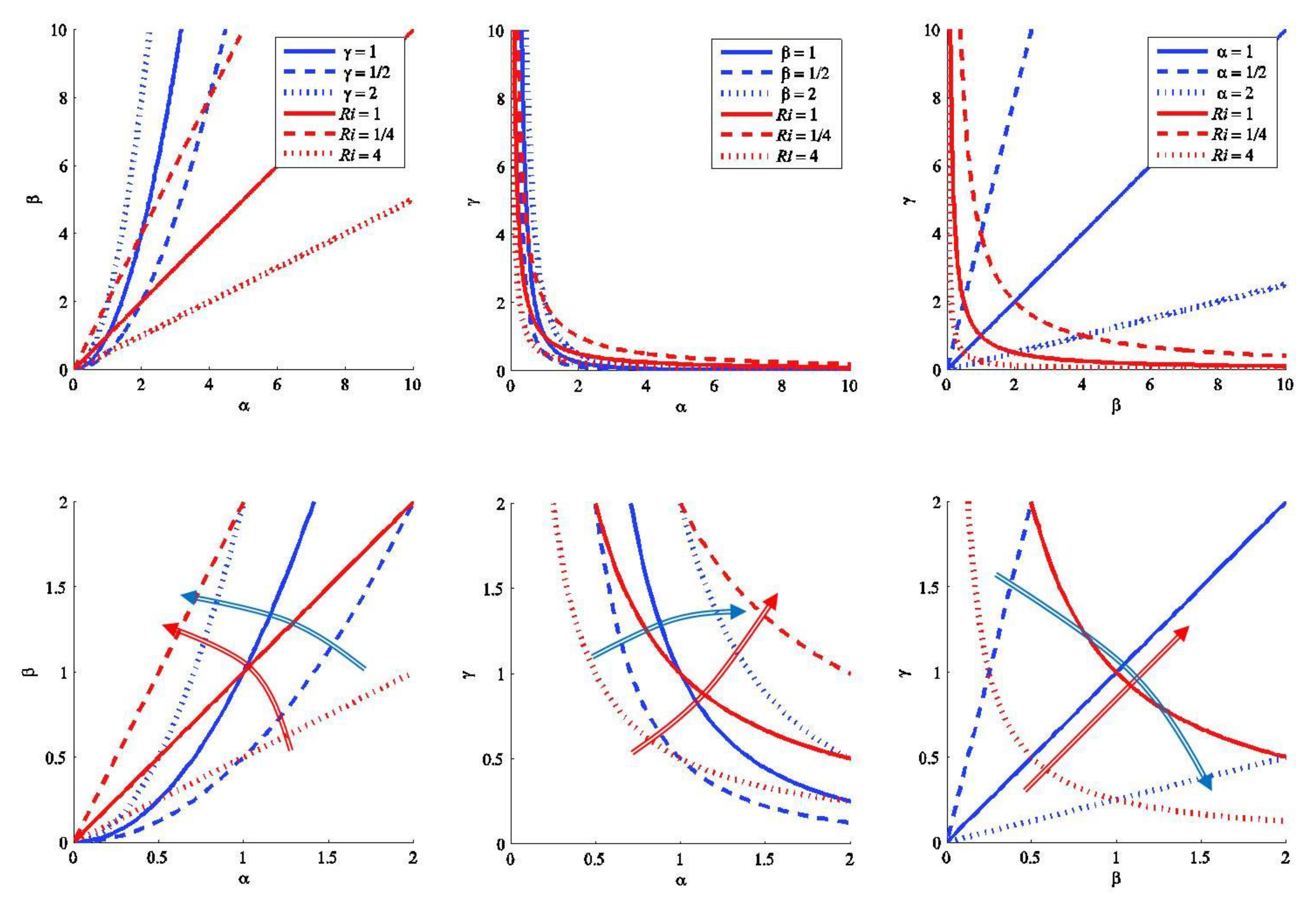
In order to clarify the dependences among the different variables, we have produced several sets of plots, where one variable is plotted as a function of another variable, for different values of the third variable and Ri (Figure 1). Specifically, we look at the following dependences (recall that

γ, α^{- 1} and β^{- 1}

refer to variables with time units):

-: for $β = β (α)$ , we have $β = γ α^{2} = (1 / {R i}^{1 / 2}) α$ ,
-: for $γ = γ (α)$ , we have $γ = β / α^{2} = (1 / {R i}^{1 / 2}) (1 / α)$ , and
-: for $γ = γ (β)$ , we have $γ = β / α^{2} = (1 / R i) (1 / β)$ .

In all these plots we show an overall perspective that goes all the way to stratification values as large as 10 times the background stratification,

α = 10

(Figure 1, upper panels), and display a close up on that region with stratification values between well mixed and twice the background stratification,

α \in [0,2]

(Figure 1, lower panels); as justified above, we are most interested on what leads to mixing in relatively well stratified conditions, e.g., for

α \in [1,2]

In the

β = β (α)

plot (Figure 1, left panels), the domain is halved in regions of supercritical and subcritical conditions, illustrating that subcritical conditions may only be reached if the vertical shear is sufficiently large,

β \geq α

. For low stratification values, subcritical conditions can only be attained for relatively large diapycnal shears (equation 8), e.g.

γ \geq 2

when

α \leq 0.5

; however, as stratification increases we find that subcritical conditions are achieved with a progressively smaller diapycnal shear, e.g. when

α \geq 2

it is sufficient to have

γ \leq 0.5

The

γ = γ (α)

plot (Figure 1, middle panels) shows a quite different partition between subcritical and supercritical conditions, which is the result of the quadratic inverse dependence of Ri on both stratification and diapycnal shear (equation 9). Only a small portion of the domain corresponds to supercritical conditions, tending to zero as either α or γ get large. In particular, for well stratified conditions the domain of subcritical conditions reaches moderate and even low diapycnal shears, necessarily coincident with high values of vertical shear.

Finally, the

γ = γ (β)

representation (Figure 1, right panels) shows the inverse linear dependence of Ri on both vertical and diapycnal shear (equation 10), with subcritical conditions requiring sufficiently large values of either one or both variables, depending on the size of vertical stratification. In particular, subcritical flow requires only moderate diapycnal shear during high stratification conditions.

The principal idea arising from all plots in Figure 1 is that moderate diapycnal shear in well stratified conditions is a guarantee for actual mixing of distinct waters. We may further explore this idea by examining the dependence of the non-dimensional reduced squared shears as a function of the squared stratification

α^{2}

for different β, γ and Ri values; for the reduced squared vertical shear

σ^{2}

we have

β^{2} - α^{2} = (γ^{2} α^{2} - 1) α^{2} = α^{2} (1 - R i) / R i

, and for the reduced squared diapycnal shear

{σ_{ρ}}^{2}

we obtain

γ^{2} - 1 / α^{2} = (β^{2} - α^{2}) α^{4} = (1 - R i) / (α^{2} R i)

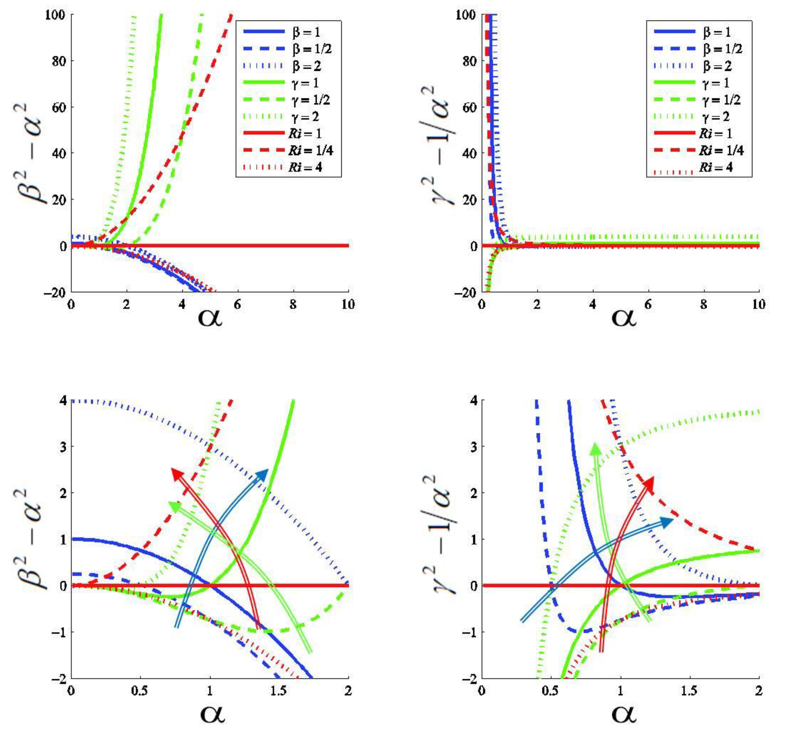
. The corresponding plots are shown in Figure 2, again up to

α = 10

(upper panels) and for

α \in [0,2]

(lower panels). Recall that subcritical conditions correspond to positive values of either reduced squared shear.

The plots for the reduced squared vertical shear (Figure 2, left panels) illustrate that one same Richardson number may correspond to many different

σ^{2}

values, each of them with a different combination of α, β, and γ values (except Ri = 1 which corresponds to

σ^{2} = 0

). In particular, positive values of

σ^{2}

are obtained under highly stratified conditions for moderate and even low diapycnal shear but require high values of vertical shear; for example, a value as low as

γ = 0.5

guarantees the subcritical conditions for

α \geq 2

, implying

β \geq 2

The plots for the reduced squared diapycnal shear (Figure 2, right panels) serve to emphasize the idea that during well stratified conditions vertical instability and mixing will only occur if the vertical shear is very high but yet a small diapycnal shear will do. In particular, for relatively large stratifications the approximation

γ^{2} - 1 / α^{2} ≅ γ^{2}

holds, i.e.

{σ_{ρ}}^{2} ≅ {S_{ρ}}^{2}

, which means that the diapycnal shear is a good stability index. In these conditions the natural oscillation time is large enough to guarantee that the flow deformation will create the instability.

In the following sections we will use three very different data sets to explore the relevance of the isopycnic perspective. Our approach will be empirical: we will display the cloud points in plots of the sort shown in Figure 1 and Figure 2, and will look for patterns of behavior for each dynamical system.

4. Data Sets

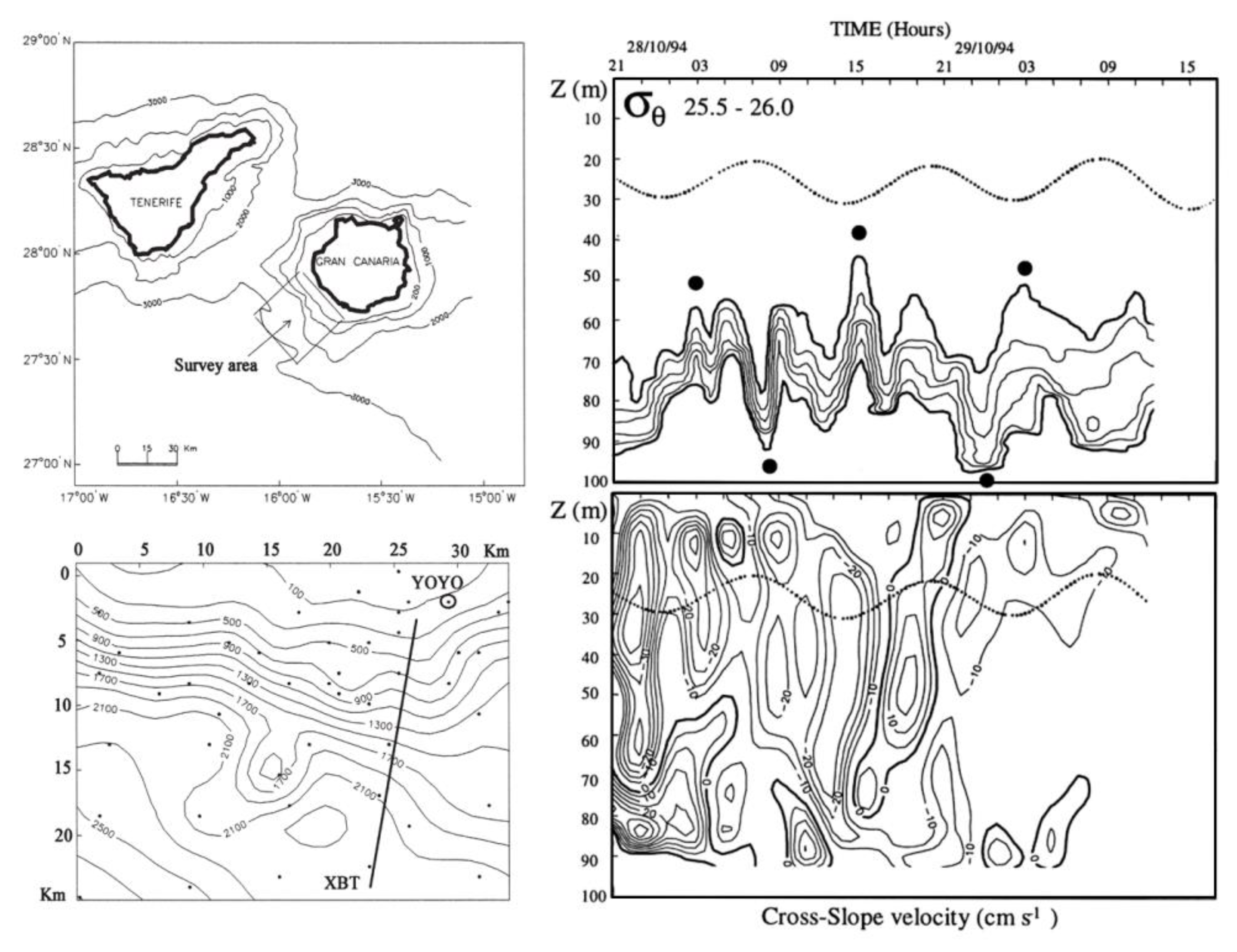
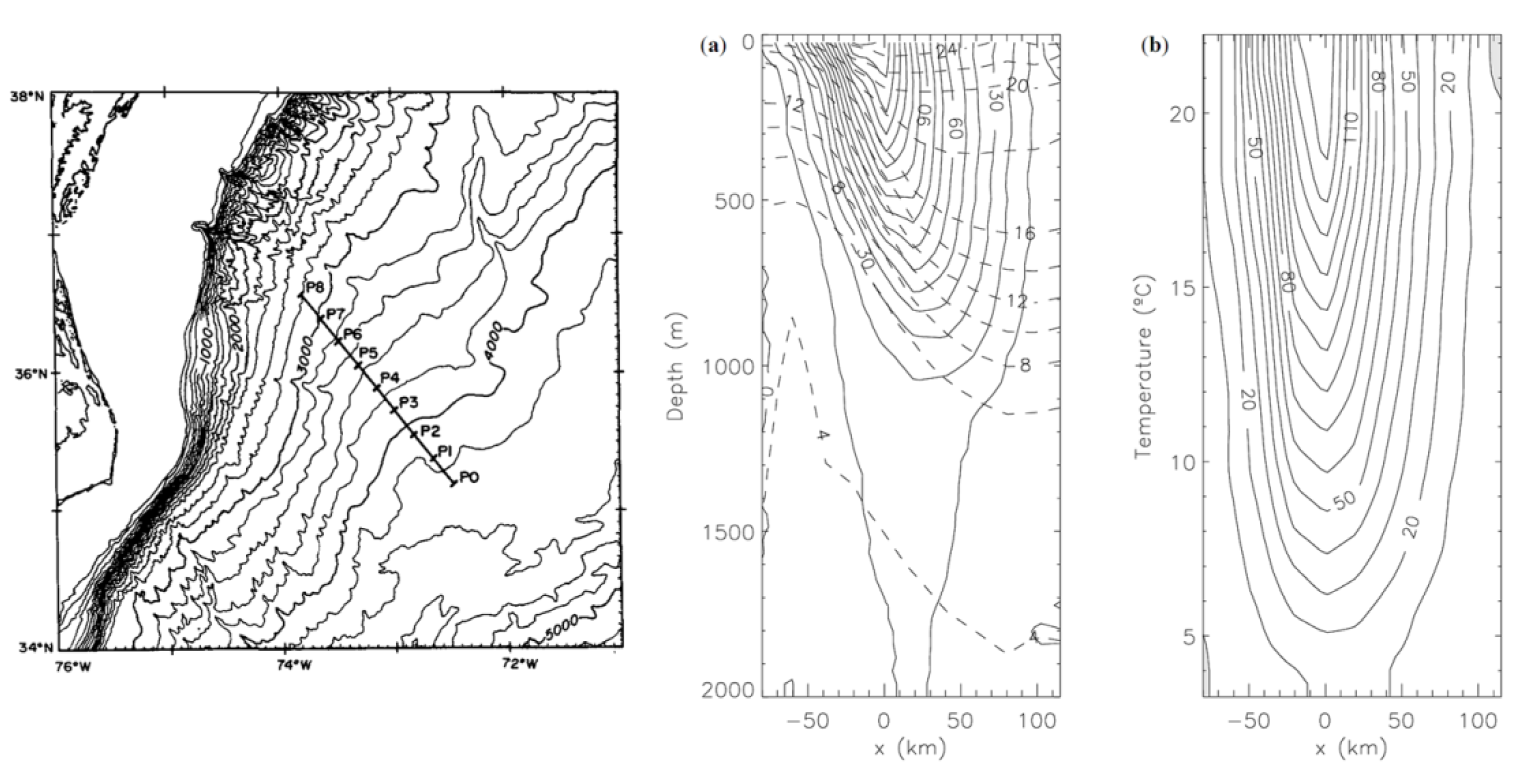
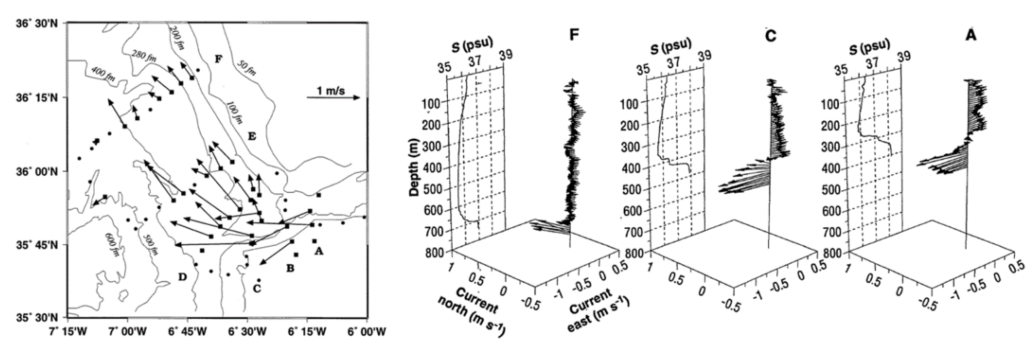
For our analysis we use three different data sets, representing very diverse oceanographic settings and dynamic conditions: (1) the shelf break of Gran Canaria Island (GCI), a deep-ocean island where internal waves are commonly present over the slope and shelf break (Figure 3); (2) the Gulf Stream (GS), an intense western boundary baroclinic current (Figure 4); and (3) the Mediterranean outflow (MO), a density-driven intense jet (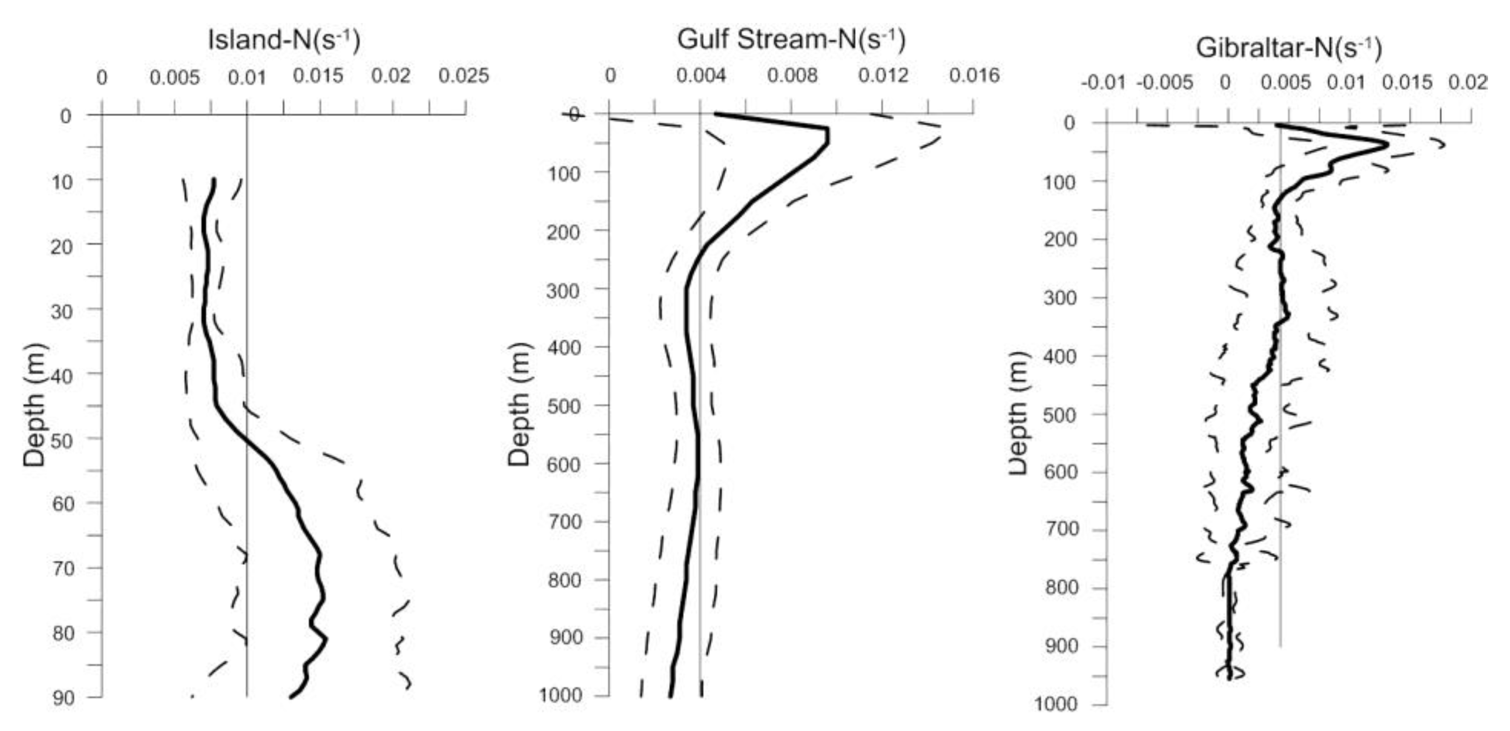Figure 5). All three data sets share the characteristic that a significant fraction of the data corresponds to well-stratified waters (Figure 6) which are experiencing an intense flow. Further, in all cases the velocity field is not inferred but actually sampled, therefore allowing a good assessment of vertical and diapycnal shears. Therefore, these data sets may be quite useful for examining the relationships between stratification, vertical shear and diapycnal shear and to explore how the Richardson number and the reduced squared (vertical and diapycnal) shears change with stratification.

The first set of data corresponds to repeated vertical sampling in the shelf break, at a fixed location on the 100-m isobath, south of GCI in fall 1994 (Sangrà et al., 2001). Sampling consisted of a ME conductivity-temperature-depth (CTD) probe which included an acoustic Doppler current-meter (Figure 3a). Density and velocity data were obtained at 1-m intervals through the water column, from near the sea surface down to the sea floor; a vertical profile was obtained every hour during nearly four days, two days of neap tides and two days of spring tides, for a total of about 9,000 samples.

Gran Canaria Island has a steep slope (about 0.15) that goes down to depths over 2500 m (Figure 3a). The dominant semidiurnal tide propagates northwards into the island steep slope and, as a result of the interaction, packets of internal waves with semidiurnal and higher periodicities are generated. The structure of the water column consisted of a surface mixed layer, a 20 to 30 m thick seasonal thermocline where the potential-density anomaly increased from 1025.5 to 1026.0 kg m^-3, and a relatively thin bottom mixed layer (Figure 3). The buoyancy frequency shows a fairly well-mixed region in the upper half of the water column on top of varyingly stratified waters in the bottom half, with a mean buoyancy frequency equal to 0.010 s^-1 (Figure 6). The cross-slope velocities often exceeded 0.2 m s^-1 in the entire water column, leading to subcritical conditions not only in the mixed layers but also in the thermocline (Figure 3b) (Sangrà et al., 2001).

The second data set consists of 20 repeated hydrographic sections across the GS, carried out between September 1980 and May 1983. These sections have temperature data obtained with expendable bathythermographs (XBT) and velocity data obtained from free-falling Pegasus instruments (Spain et al., 1981); the data were originally reported and analyzed by Halkin and Rossby (1985), see also Ratsimandresy and Pelegrí (2005) and references therein (Figure 4a). The temperature values were converted into potential density data by means of a recursive utilization of Armi and Bray’s (1982) algorithms, as explained in Rodríguez-Santana et al. (1999). Each section contained between four and ten stations of velocity and potential density from the sea surface down to 2000 m at 25-m intervals, for a total of some 10,000 samples.

The permanent thermocline of the GS, with temperatures between about 6 and 16ºC, slope sharply towards the continental slope, raising some 600-700 m in 100 km. As a result, the GS velocities increase from about 0.25 to over 1.5 m s^-1 over this same temperature range; on both sides of the GS the mean vertical stratification remains similar but the velocities are substantially smaller (Figure 4b). The relatively low vertical data resolution limits the sampling of high-shear events associated to internal waves, which would be responsible for a significant increase in the gradient Richardson values, and hence restricts our analysis to near-geostrophic flow (Van Gastel and Pelegrí, 2004). Despite so, the background geostrophic velocity field is intense enough for the core of the GS to experience several instances of subcritical conditions (Ri < 1) which are responsible for vertical mixing (Pelegrí and Csanady, 1991, 1994). The buoyancy frequency decreases largely in the top 300 m and remains approximately constant down to 1000 m, with low variability characteristic for the subtropical permanent thermocline; the mean background stratification for this second data set is 0.004 s^-1 (Figure 6).

The third set of data consists of 56 stations, with full-depth CTD profiles and simultaneous velocity measurements with expendable current profilers (XCP), sampled in the eastern Gulf of Cádiz during fall 1988 (Price et al., 1993; Baringer and Price, 1997a,b); about half of the stations sampled the MO (Figure 5). Velocity and density data were recorded every 2 m; for an average depth of about 500 m, this represents some 14,000 data points.

As the MO exits the Strait of Gibraltar, over a distance of less than 50 km, it experiences three different dynamic regions. In the first phase, located between Spartel Sill (360 m) and Western Spartel Sill (420 m, located at about 6º20’W, 35º47’N), the MO follows west along a relatively narrow (about 5 km wide) and gently sloping channel, the water depth increasing between 360 and 420 m in about 20 km. In the second phase, the MO continues west along a channel of variable amplitude (typically 5 to 10 km) and undergoes three abrupt topography-driven accelerations (a total depth change from 420 to 700 m over a distance of another 20 km) with core velocities in excess of 1 m s^-1, resulting in substantial dilution. During these two phases the MO approximately occupies the bottom third of the water column. In the third phase the MO follows northwest, its diluted core moving with much slower velocities, leaning against the Iberian continental slope (Price et al., 1993; Gasser et al., 2011, 2017; Nash et al., 2012). Therefore, the local profile of the buoyancy frequency depends on whether the station is close to Gibraltar and whether it is found on the path or away from the path of the MO; for this reason the variability is largest between 200 and 750 m, and decreases in the bottom 100 m simply as a reflection of the few stations we are using for deep waters, the mean buoyancy frequency is 0.004 s^-1 (Figure 6).

5. Results

We non-dimensionalize the variables as explained in section 3, with the mean buoyancy frequencies for each data set as shown in Table 1. Using one single background buoyancy frequency for an individual data set allows taking into consideration the dynamic changes within one single region; additionally, the utilization of different background stratifications (one per region) facilitates a unified interpretation of all three, potentially quite different, cases.

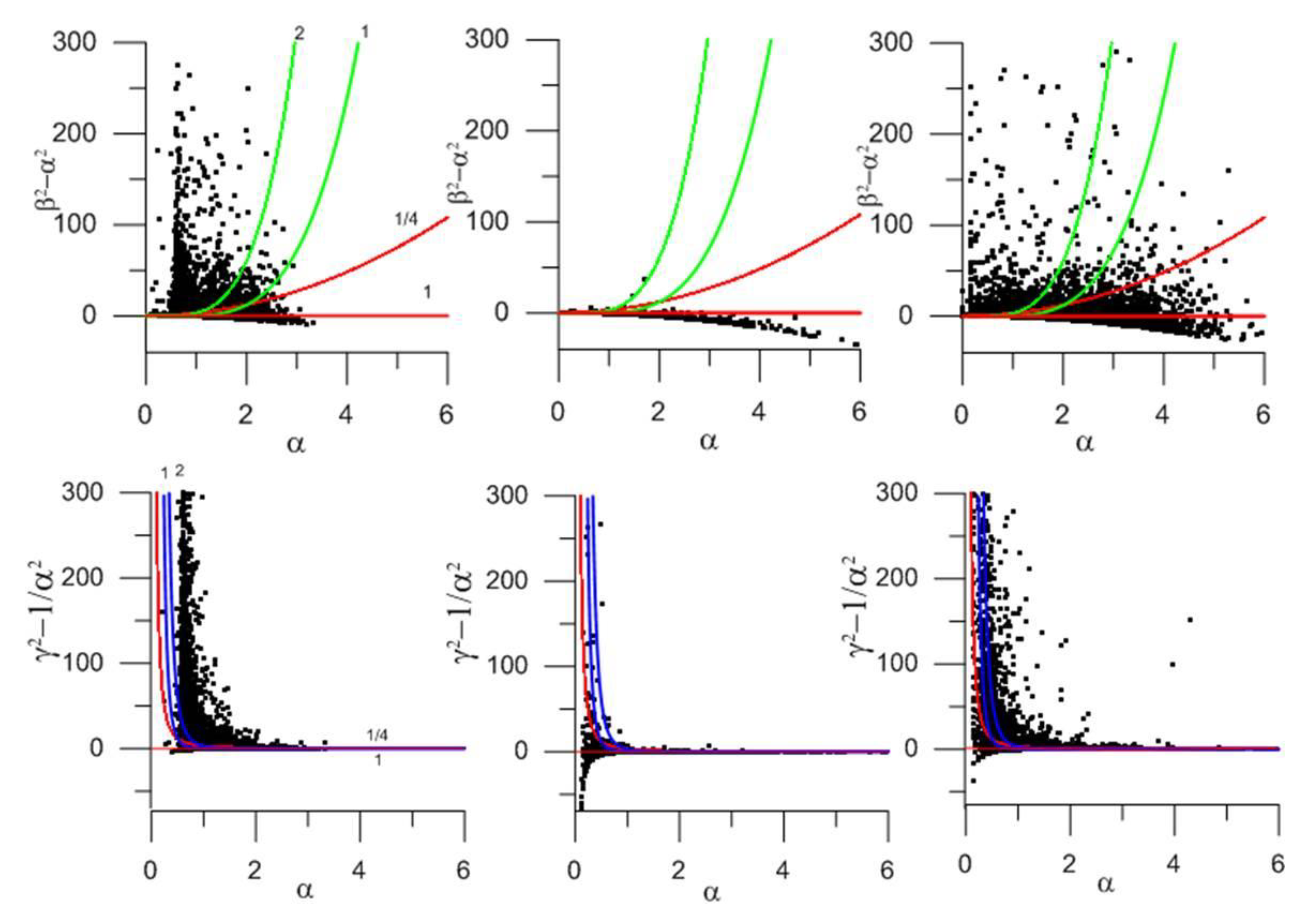
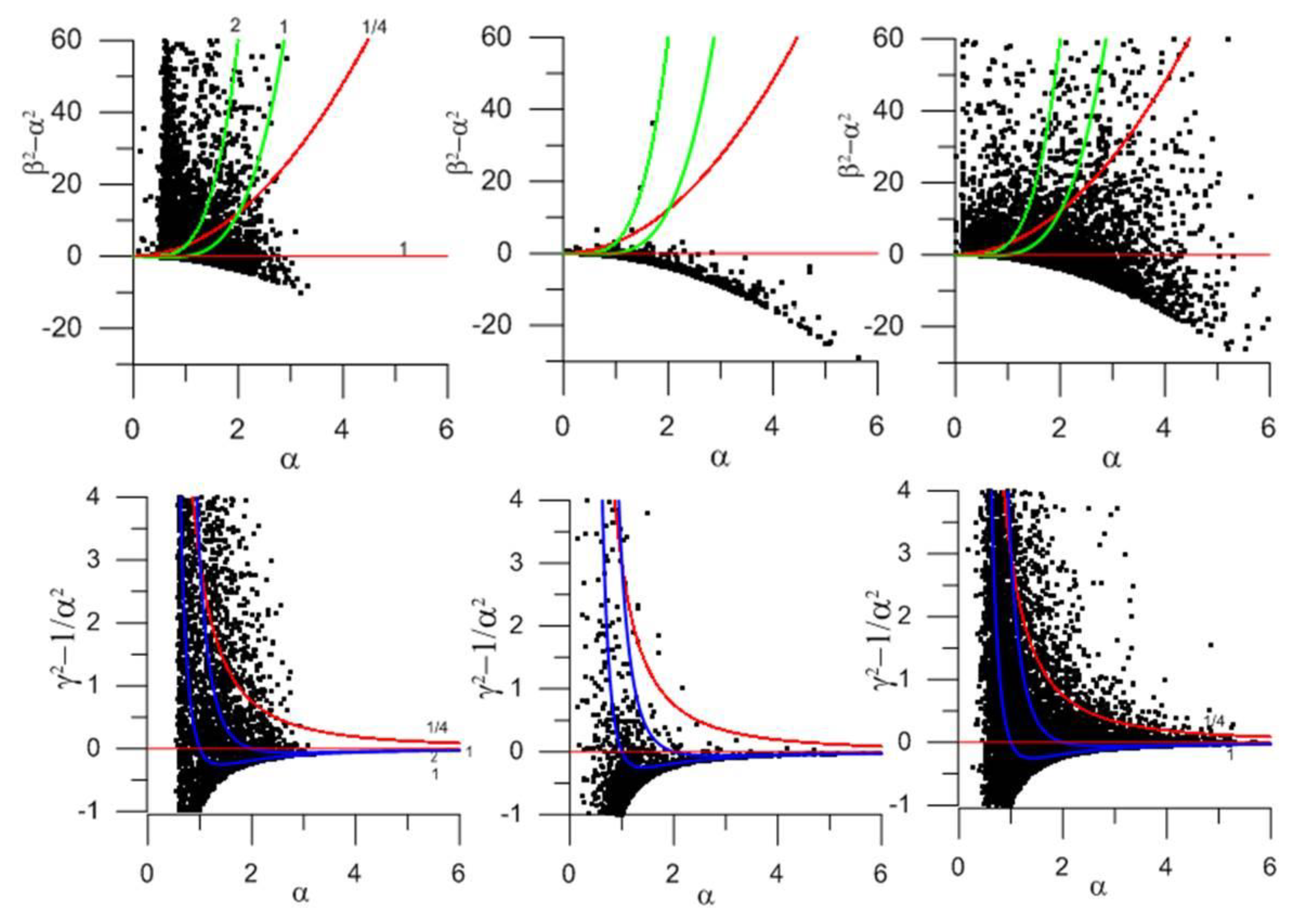
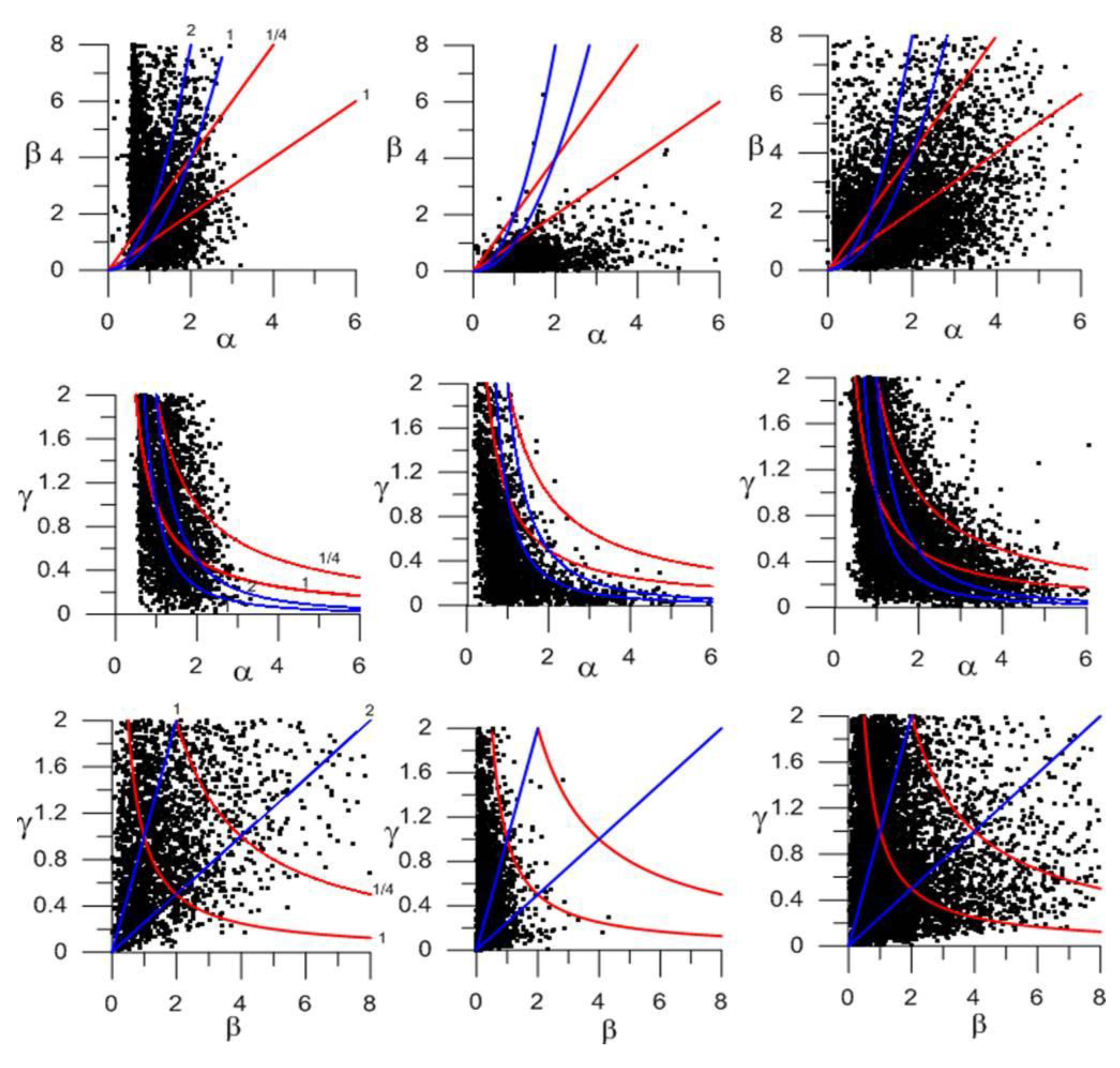
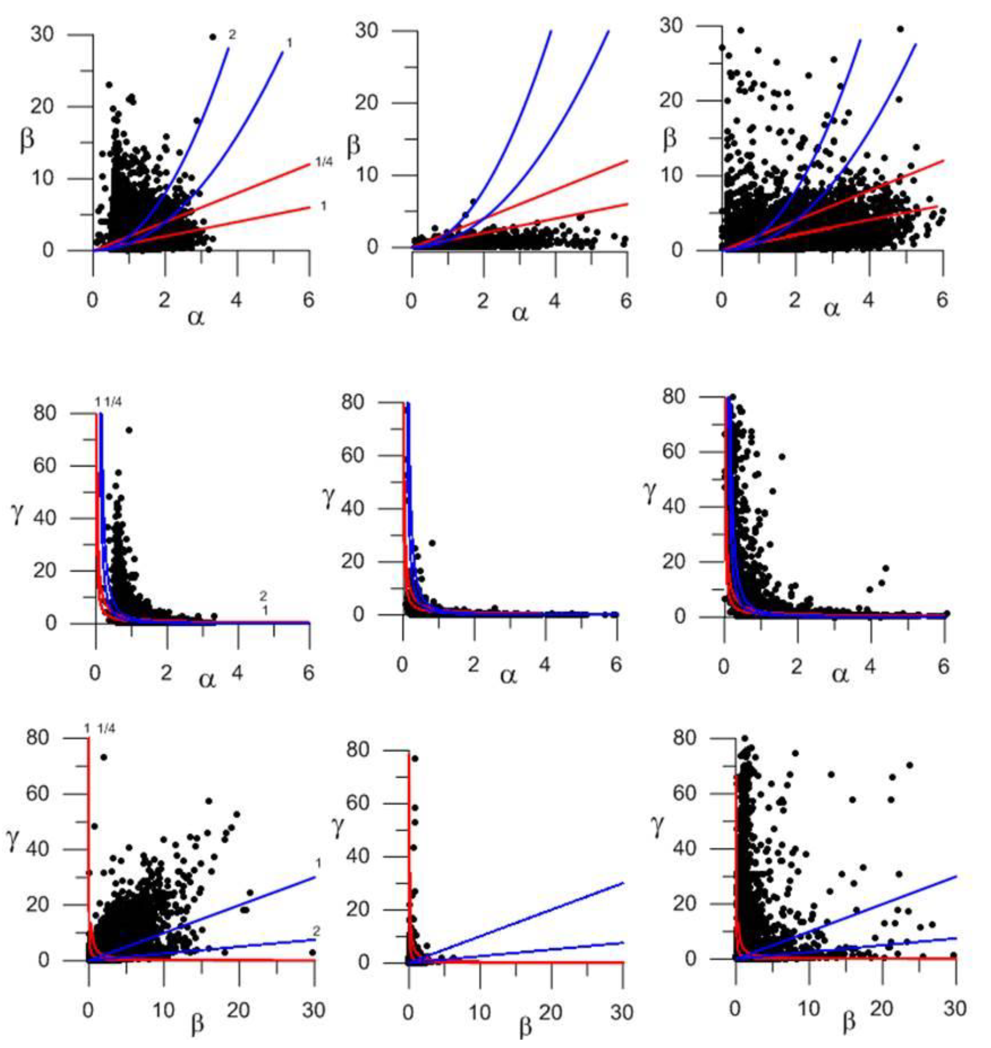
Consider first the cloud points for all three original variables (vertical stratification, vertical shear, diapycnal shear; Figure 7), in particular the zoom for the high stratification and high shear domain (Figure 8). The overall shape of the

β = β (α)

representation changes greatly among all three cases, with no noticeable dependence of vertical shear on stratification. The common denominator for all three cases is that β takes a relatively high range of values for any α (Figure 8 and Figure 9, top panels). In contrast, all

γ = γ (α)

cloud points have similar shapes, with relatively high values and high variability at low stratification conditions and the opposite for well stratified waters (Figure 7 and Figure 8, middle panels); the cloud points actually suggest a decay of the maximum diapycnal shears with increasing vertical stratification. Finally, the

γ = γ (β)

plots again display very large differences between all three cases, with the Island and Gulf Stream cases displaying completely different distributions and the MO possibly as an intermediate situation (Figure 7 and Figure 8, bottom panels).

These results may be interpreted as if each flow has its own dynamics, setting a range of characteristic diapycnal shears. We may step forward and see if this dynamics is reflected in some controlling parameter. In section 2 we argued the reduced squared diapycnal shear,

{σ_{ρ}}^{2}

, to be such a parameter. This variable is an index for the stability of the system, in the same way as the Richardson number, but with the advantage that

{σ_{ρ}}^{2}

decreases with increasing stratification, i.e., given two situations with the same Ri value, we may identify those leading to more effective mixing as those with lower

{σ_{ρ}}^{2}

values. Another advantage is that

{σ_{ρ}}^{2}

has a maximum value equal to the squared diapycnal shear itself

{S_{ρ}}^{2}

, to be attained during high stratification conditions. For a number of situations where the flow has some characteristic dynamics, such as the frontogenetic situation described in section 2.1, the maximum value of

{σ_{ρ}}^{2}

will be conditioned by the initial flow and the evolving stratification. These ideas are sustained by the cloud points of

σ^{2}

and

{σ_{ρ}}^{2}

as a function of stratification (Figure 9 and Figure 10). The distribution of

σ^{2}

is quite different for each case, with large scattering for all α; in contrast, the distribution of

{σ_{ρ}}^{2}

does hint at a dependence with α, with its maximum values decreasing with increasing stratification.

In order to further examine these ideas, we look at the way the mean values and standard deviations of all three stability indices (

R i

σ^{2}

and

{σ_{ρ}}^{2}

) change with stratification (Figure 11; for this calculation the mean values and standard deviations are calculated over 0.2 intervals of α). The results indeed show no clear relation of

σ^{2}

and Ri with stratification. However, they do suggest the existence of a univocal dependence of

{σ_{ρ}}^{2}

with stratification for each particular flow; this dependence changes from one case to another, it being a direct relation for the GCI shelf break and MO cases and an inverse one for the GS data.

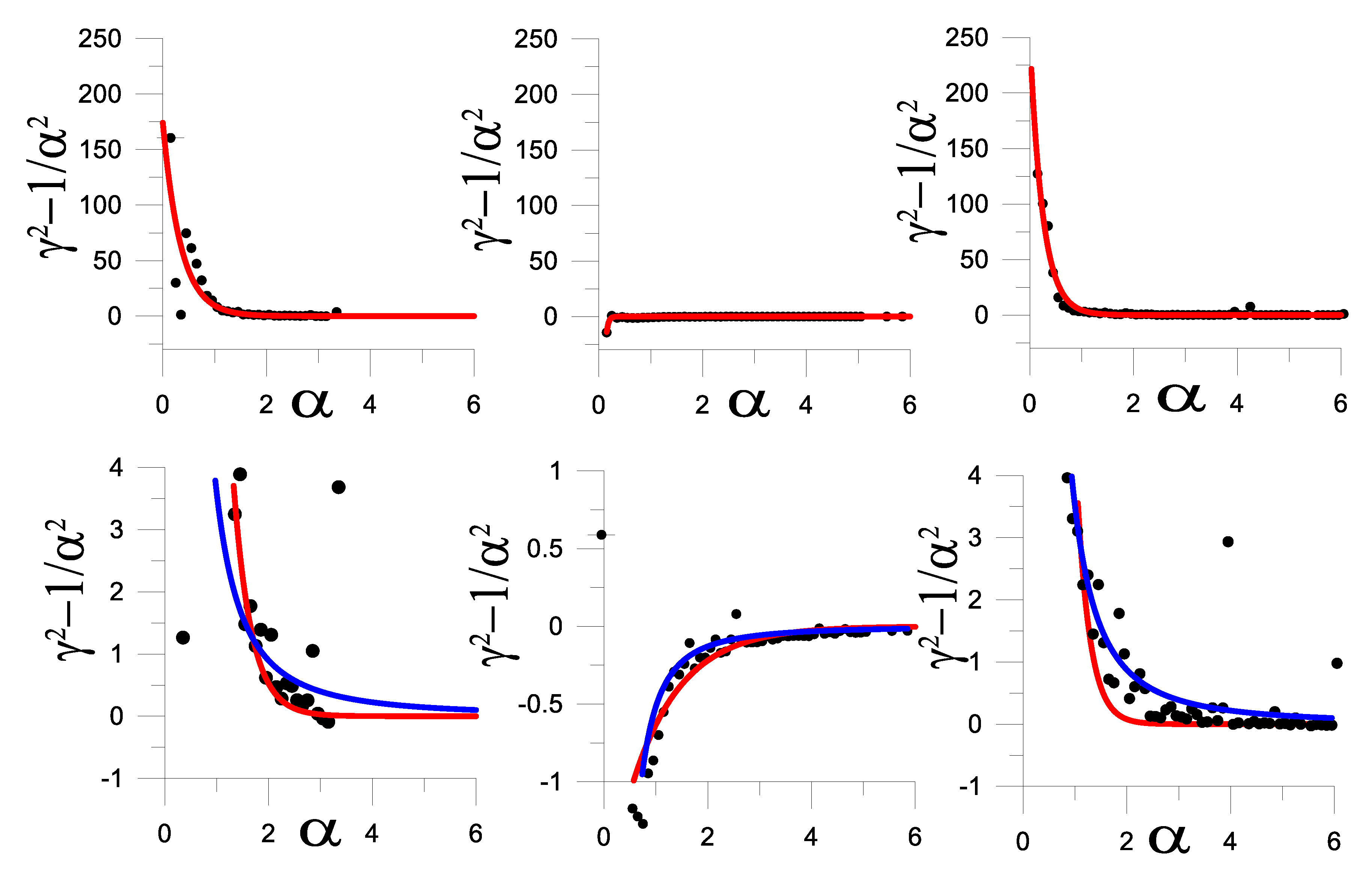
Finally, we explore if there are simple functions that can provide a good fit to the observed mean

{σ_{ρ}}^{2} (α)

dependence (Figure 12; mean values are now calculated over 0.1 α intervals). Our first attempt is the simple exponential decay with stratification, given by

{σ_{ρ}}^{2} = {σ_{0}}^{2} e x p (- r α)

. It turns out that the adjustment is fairly good for all cases, with the best-fit parameters (as calculated separately for each data set) presented in Table 1; notice that, because of the excellent fit for low and high values of α and despite of some misfit in the interval

α \in [1.5,2.5]

, the highest correlation with the data corresponds to the MO case. For GCI and MO the exponential coefficient is relatively large (2.90 and 4.03) as compared with the one for the GS (1.05); the main difference, however, is that for GCI and MO the mean

{σ_{ρ}}^{2}

values remain always positive, indicative of unstable conditions, while for GS they are negative.

An equally good

{σ_{ρ}}^{2} (α)

fit corresponds to the dependence given by equation (7), its non-dimensional form being

{σ_{ρ}}^{2} = (1 - R i) / (α^{2} R i)

, for constant Ri values. Again in this adjustment we may appreciate a similar behavior for GCI and MO, quite different from what happens for the GS. In the former cases the best fit corresponds to a subcritical Ri = 0.22, while in the latter it reflects a supercritical flow with

R i

= 2.1 (Table 1); it is remarkable that this happens despite the mean Richardson values are almost always significantly greater than one (top panels of Figure 11). Our interpretation is that, despite all the variability reflected by the scattered points in Figure 10, each case responds to a different flow dynamics which can be characterized by a

{σ_{ρ}}^{2} (α)

dependence that is set uniquely through a characteristic flow-dependent Ri value, in agreement with the idea that strongly stratified flow self-organizes around some local critical state (Zhou, 2022).

6. Conclusions

In this work we have endorsed the advantages of isopycnic thinking for a better understanding of those conditions leading to effective mixing in stratified sheared flows. A non-dimensional analysis, in terms of the background stratification, proves to be useful to understand the interdependences between stratification, vertical shear, diapycnal shear and the Richardson number. In particular, we have discussed vertical instability in terms of characteristic times, showing that instability occurs when the natural oscillation time associated to the diapycnal shear is longer than the vertical oscillation time, which itself is longer than the deformation time.

The gradient Richardson number

R i

is the classical index to assess the occurrence of instability but it cannot differentiate between those instances when mixing effectively redistributes density (and other properties, which occurs when stratification is high) from those cases when instabilities simply displace water which is already homogeneous. Here we have extended the work from Kunze et al. (1990) and Sun et al. (1998) by defining the reduced squared vertical shear

σ^{2}

(in vertical coordinates) and the reduced squared diapycnal shear

{σ_{ρ}}^{2}

(in isopycnic coordinates). The three indices for instability (Ri,

σ^{2}

and

{σ_{ρ}}^{2}

) are sensitive to stratification but

{σ_{ρ}}^{2}

has the special property of decreasing with increasing stratification, for either constant or variable

R i

values, towards a limiting value equal to the squared diapycnal shear

{S_{ρ}}^{2}

We have finally examined the distribution of the non-dimensional variables and indices for three quite different dynamic regimes: a shelf break characterized by intense internal waves, the highly baroclinic Gulf Stream, and the gravity-current Mediterranean outflow. The most remarkable feature is the decay of both the mean and maximum

{S_{ρ}}^{2}

and

{σ_{ρ}}^{2}

values with increasing stratification, which changes for each different flow regime, endorsing the idea that

{σ_{ρ}}^{2} > 0

is a good index for assessing the flow stability:

{σ_{ρ}}^{2}

has to be large for low stratification values but small positive values are sufficient for high stratification. The non-dimensional expression

{σ_{ρ}}^{2} = (1 - R i) / (α^{2} R i)

adjusts well to the mean

{σ_{ρ}}^{2} (α)

experimental values, leading to a family of instability functions with one characteristic Ri value for each flow regime.

Author Contributions

Funding

Acknowledgments

The authors wish to sincerely thank Tom Rossby and Jim Price for respectively sharing the Gulf Stream and Mediterranean outflow data sets. This work has been funded by the Spanish Government through Project SACO (Ministerio de Ciencia e Innovación, reference PID2022-139403NB-C22). MC is grateful to the MSCA programme, funded by the European Union (HORIZON-MSCA-2021-PF MOORING, grant agreement no. 101064423). This article is a publication of the Unidad Océano y Clima of the Universidad de Las Palmas de Gran Canaria, an R+D+I CSIC-associate unit. The authors also recognize the institutional support of the Spanish Government through the Severo Ochoa Center of Excellence accreditation (CEX2019-000928-S).

Conflicts of Interest

References

Abarbanel, H. D. I., D. D. Holm, J. E. Mardsen, and R. Ratiu, 1984. Richardson number criterion for the nonlinear stability of three-dimensional stratified flow. Phys. Rev. Lett., 52, 2352-2355.
Abarbanel, H. D. I., D. D. Holm, J. E. Mardsen, and R. Ratiu, 1986. Nonlinear stability analysis of stratified fluid equilibria. Phil.Trans. R. Soc. Lond., 318, 349-409.
Baringer, M. O., and J. F. Price, 1997a. Mixing and spreading of the Mediterranean outflow. J. Phys. Oceanogr., 27, 1654–1677. [CrossRef]
Baringer, M. O., and J. F. Price, 1997b. Momentum and energy balance of Mediterranean outflow. J. Phys. Oceanogr., 27, 1678–1692. [CrossRef]
Cisneros-Aguirre, J., J. L. Pelegrí, and P. Sangrà, 2001. Experiments on layer formation in stratified shear flow. Sci. Mar., 65(S1), 117-126. [CrossRef]
Gasser, M., J. L. Pelegrí, J. Nash, H. Peters, and J. García-Lafuente, 2011. Topographic steering of the early plunging Mediterranean outflow. Geo-Mar. Lett., 31, 301-314.
Gasser, M., J. L. Pelegrí, M. Emelianov, M. Bruno, E. Gracia, M. Pastor, H. Peters, A. Rodríguez-Santana, and J. Salvador, 2017. Tracking the Mediterranean outflow in the Gulf of Cádiz. Progr. Oceanogr., 157, 47-71. [CrossRef]
Grachev, A. A., E. L. Andreas, C. W. Fairall, P. S. Guest, and P. O. G. Persson, 2013. The critical Richardson number and limits of applicability of local similarity theory in the stable boundary layer, Boundary Layer Meteorol., 147, 51–82. [CrossRef]
Halkin, D., and T. Rossby, 1985. The structure and transport of the Gulf Stream at 73°W. J. Phys. Oceanogr., 15, 1439-1452. [CrossRef]
Hazel, P. G., 1972. Numerical studies of the stability of inviscid parallel shear flows. J. Fluid Mech., 51, 39-62.
Howard, L. N., 1961. Note on a paper of John W. Miles. J. Fluid Mech., 10, 509-512. [CrossRef]
Kunze, E., A. J. Williams, and M. G. Briscoe, 1990. Observations of shear and vertical stability from a neutrally buoyant float. J. Geophys. Res., 95, 18127-18142. [CrossRef]
Miles, J. W., 1961. On the stability of heterogenous shear flows. J. Fluid Mech., 10, 496-508. [CrossRef]
Miles, J. W., 1986. Richardson’s criterion for the stability of stratified shear flow. Phys. Fluids, 29, 3470-3471. [CrossRef]
Nash, J. D., H. Peters, S. M. Kelly, J. L. Pelegrí, M. Emelianov, and M. Gasser, 2012. Turbulence and High-Frequency Variability in a Deep Gravity Current Outflow. Geophys. Res. Lett. 39, L18611. [CrossRef]
Pelegrí, J. L. and G. T. Csanady, 1994. Diapycnal mixing in western boundary currents. J. Geophys. Res., 99, 18275-18304. [CrossRef]
Pelegrí, J. L., and P. Sangrá, 1998. A mechanism for layer formation in stratified geophysical flows. J. Geophys. Res., 103, 30679-30693. [CrossRef]
Pelegrí, J. L., A. Rodríguez-Santana, P. Sangrá, and A. Marrero-Díaz, 1998. Modeling of shear-induced diapycnal mixing in frontal systems. Appl. Sci. Res., 59, 159-175. [CrossRef]
Price, J. F., M. O. Baringer, R. G. Lueck, G. C. Johnson, I. Ambar, G. Parrilla, A. Cantos, M. A. Kennelly, and T. B. Sanford, 1993. Mediterranean outflow mixing and dynamics. Sci., 259, 1277–1282. [CrossRef]
Ratsimandresy, A. W., and J. L. Pelegrí, 2005. Vertical alignment of the Gulf Stream. Tellus A, 57, 691-700.
Rodríguez-Santana, A., J. L. Pelegrí, P. Sangrà, and A. Marrero-Díaz, 1999. Diapycnal mixing in Gulf Stream meanders. J. Geophys. Res., 104, 25891-25912. [CrossRef]
Roget, E., J. L. Pelegrí, J. Planella-Morató, J. Puigdefàbregas, M. Emelianov, I. Vallès-Casanova, and D. Orúe-Echevarria, 2023. Diapycnal mixing in the Brazil-Malvinas confluence front. Progr. Oceanogr., 211, 102968. [CrossRef]
Sangrà, P., G. Basterretxea, J. L. Pelegrí, and J. Arístegui, 2001. Chlorophyll increase by internal waves in the shelf-break of Gran Canaria (Canary Islands). Sci. Mar., 65(S1), 89-97. [CrossRef]
Spain, P. F., D. L. Dorson, and H. T. Rossby, 1981. PEGASUS, a simple, acoustically tracked, velocity profiler. Deep-Sea Res., 28, 1553-1567.
Sun, C., W. D. Smyth, and J. N. Moum, 1998. Dynamic instability of stratified shear flow in the upper equatorial Pacific. J. Geophys. Res., 103, 10323-10337. [CrossRef]
Taylor, G. I., 1931a. Effect of variation in density on the stability of superposed streams of fluid. Proc. R. Soc. London A, 132, 499-523. [CrossRef]
Taylor, G. I., 1931b. Internal waves and turbulence in a fluid of variable density. Rapp. P-v réun.-Cons. int. explor. Mer, 76, 35-43.
Van Gastel, P., and J. L. Pelegrí, 2004. Estimates of gradient Richardson numbers from vertically smoothed data. Sci. Mar., 68, 459-482.
Zhou, Q., 2022. Threshold behavior of local gradient Richardson number in strongly stratified nonequilibrium turbulence. Phys. Rev. Fluids, 7, 104802. [CrossRef]

Figure 1. (Left panels) Vertical shear as a function of stratification

β = β (α)

, (middle panels) diapycnal shear as a function of stratification

γ = γ (α)

, and (right panels) diapycnal shear as a function of vertical shear

γ = γ (β)

. Red curves stand for different Ri values and blue curves for different values of the third variable; the dashed, solid and dotted lines respectively correspond to values less, equal and greater than one. In the top panels we present the results in the [0:10, 0:10] domain, while in the bottom panels we zoom at the [0:2, 0:2] domain; the colored arrows illustrate the direction for Ri decreasing (all panels), γ increasing (left), β increasing (center) and α increasing (right).

Figure 1. (Left panels) Vertical shear as a function of stratification

β = β (α)

, (middle panels) diapycnal shear as a function of stratification

γ = γ (α)

, and (right panels) diapycnal shear as a function of vertical shear

γ = γ (β)

Figure 2. (Left panels) Non-dimensional reduced squared vertical shear

β^{2} - α^{2}

and (right panels) reduced squared diapycnal shear

γ^{2} - 1 / α^{2}

, in both cases plotted as a function of stratification α. Red curves stand for different Ri values, blue curves for different β values, and green curves for different γ values; the dashed, solid and dotted lines respectively correspond to values less, equal and greater than one. In the top panels we present the results in the [0:10, 0:100] domain, while in the bottom panels we zoom at the [0:2, 0:4] domain; the colored arrows illustrate the direction where the flow becomes subcritical (Ri decreasing) and the shear increases.

Figure 2. (Left panels) Non-dimensional reduced squared vertical shear

β^{2} - α^{2}

and (right panels) reduced squared diapycnal shear

γ^{2} - 1 / α^{2}

Figure 3. (Top left) Survey area southwest of Gran Canaria Island. (Bottom left) Bathymetry with the YOYO station at the shelf-break. (Right panels) Time-depth plots of two days of density and velocity measurements. Top: barotropic tide (dotted line, amplified by a factor of 10) and pycnocline (solid lines; isopycnals at 0.1 intervals, with 25.5 and 26.0 shown as bold contours); bottom: cross-slope speed, with positive onshore values. Reproduced from Sangrà et al. (2001).

Figure 4. (Left panel) Location of the velocity and temperature stations (P0 through P8) across the Gulf Stream, off the east coast of North America, with the bottom isobaths. Reproduced from Halkin and Rossby (1985). (Central panel) Vertical section of the mean velocity and temperature fields, and (right panel) velocity plotted as a function of temperature. Reproduced from Ratsimandresy and Pelegrí (2005).

Figure 5. (Left panel) Location of most stations with conductivity and velocity data that have been used in our analysis, with vectors illustrating the maximum observed outflow velocity; some additional stations inside the Strait of Gibraltar are not shown. (Right panel) Examples of velocity and salinity profiles along the outflow axis of sections A, C and F (see left panel for the location of each section). Reproduced from Price et al. (1993).

Figure 6. Buoyancy frequency as a function of depth for the measurements at (left) the shelf break of Gran Canaria Island, (middle) the Gulf Stream permanent thermocline, and (right) the region west of Gibraltar which includes the Mediterranean outflow. The solid lines represent the mean profiles while the dashed lines indicate the one-standard deviation limit from this mean profile.

Figure 7. Scattered data plot of (top panels)

β = β (α)

, (center panels)

γ = γ (α)

, and (bottom panels)

γ = γ (β)

for the three data sets: (left panels) island shelf break, (middle panels) Gulf Stream, and (right panels) Mediterranean outflow. The red lines in the top, center, and bottom panels respectively correspond to contours of

β = α / R i

γ = 1 / (α R i)

, and

γ = 1 / (β R i)

, for Ri = 0.25 and 1. The blue lines correspond to contours of (top panels)

β = γ α^{2}

for γ = 1 and 2, (center panels)

γ = β / α^{2}

for β = 1 and 2, (bottom panels)

γ = β / α^{2}

for α = 1 and 2.

Figure 7. Scattered data plot of (top panels)

β = β (α)

, (center panels)

γ = γ (α)

, and (bottom panels)

γ = γ (β)

β = α / R i

γ = 1 / (α R i)

, and

γ = 1 / (β R i)

, for Ri = 0.25 and 1. The blue lines correspond to contours of (top panels)

β = γ α^{2}

for γ = 1 and 2, (center panels)

γ = β / α^{2}

for β = 1 and 2, (bottom panels)

γ = β / α^{2}

for α = 1 and 2.

Figure 8. As in Figure 7 but zooming at

\in [0,6]

β \in [0,8]

and

γ \in [0,2]

Figure 8. As in Figure 7 but zooming at

\in [0,6]

β \in [0,8]

and

γ \in [0,2]

Figure 9. Scattered data plot of (top panels)

β^{2} - α^{2}

and (bottom panels)

γ^{2} - 1 / α^{2}

, both as a function of α, for the three data sets: (left panels) island shelf break, (middle panels) Gulf Stream, and (right panels) Mediterranean outflow. The red lines in all panels respectively correspond to contours of

β^{2} - α^{2} = α^{2} (1 - R i) / R i

and

γ^{2} - 1 / α^{2} = (1 - R i) / (α^{2} R i)

, for Ri = 0.25 and 1. The green lines in the top panels correspond to contour of

β^{2} - α^{2} = (γ^{2} α^{2} - 1) α^{2}

for γ = 1 and 2, and the blue lines in the bottom panels correspond to contours of

γ^{2} - 1 / α^{2} = (β^{2} - α^{2}) / α^{4}

for β = 1 and 2.

Figure 9. Scattered data plot of (top panels)

β^{2} - α^{2}

and (bottom panels)

γ^{2} - 1 / α^{2}

β^{2} - α^{2} = α^{2} (1 - R i) / R i

and

γ^{2} - 1 / α^{2} = (1 - R i) / (α^{2} R i)

, for Ri = 0.25 and 1. The green lines in the top panels correspond to contour of

β^{2} - α^{2} = (γ^{2} α^{2} - 1) α^{2}

for γ = 1 and 2, and the blue lines in the bottom panels correspond to contours of

γ^{2} - 1 / α^{2} = (β^{2} - α^{2}) / α^{4}

for β = 1 and 2.

Figure 10. As in Figure 9 but zooming at

α \in [0,6]

β^{2} - α^{2} \in [- 30,60]

and

γ^{2} - 1 / α^{2} \in [- 1,4]

Figure 10. As in Figure 9 but zooming at

α \in [0,6]

β^{2} - α^{2} \in [- 30,60]

and

γ^{2} - 1 / α^{2} \in [- 1,4]

Figure 11. Mean values, together with standard deviations, for (top panels) Ri, (center panels)

β^{2} - α^{2}

, and (bottom panels)

γ^{2} - 1 / α^{2}

, as a function of α. The three columns correspond to the three data sets: (left panels) island shelf break, (middle panels) Gulf Stream, and (right panels) Mediterranean outflow.

Figure 11. Mean values, together with standard deviations, for (top panels) Ri, (center panels)

β^{2} - α^{2}

, and (bottom panels)

γ^{2} - 1 / α^{2}

, as a function of α. The three columns correspond to the three data sets: (left panels) island shelf break, (middle panels) Gulf Stream, and (right panels) Mediterranean outflow.

Figure 12. The

γ^{2} - 1 / α^{2}

mean values are plotted as a function of α; the lower panels reproduce the top panels but zooming at the (left and right panels)

γ^{2} - 1 / α^{2} \in [- 1,4]

and (middle panel)

γ^{2} - 1 / α^{2} \in [- 1,1]

intervals. The red and blue lines respectively correspond to the exponential and Ri-based adjustments to these mean values (see text for explanation). The three columns correspond to the three data sets: (left panels) island shelf break, (middle panels) Gulf Stream, and (right panels) Mediterranean outflow.

Figure 12. The

γ^{2} - 1 / α^{2}

mean values are plotted as a function of α; the lower panels reproduce the top panels but zooming at the (left and right panels)

γ^{2} - 1 / α^{2} \in [- 1,4]

and (middle panel)

γ^{2} - 1 / α^{2} \in [- 1,1]

Table 1. Background buoyancy frequency (s^-1) and best-fit parameters to the mean

{σ_{ρ}}^{2}

values for two different functions with the

R^{2}

correlation coefficients.

Table 1. Background buoyancy frequency (s^-1) and best-fit parameters to the mean

{σ_{ρ}}^{2}

values for two different functions with the

R^{2}

correlation coefficients.

		Gran Canaria Island	Gulf Stream	Mediterranean Outflow
Background N (s^-1)		0.010	0.004	0.004
best exponential adjustment ${σ_{ρ}}^{2} = {σ_{0}}^{2} e x p (- r α)$	${σ_{ρ}}^{2}$	174.2	-1.9	250.3
	r	2.90	1.05	4.03
	$R^{2}$	0.66	0.83	0.97
best adjustment as ${σ_{ρ}}^{2} = (1 - R i) / (α^{2} R i)$	Ri	0.217	2.067	0.222
best adjustment as ${σ_{ρ}}^{2} = (1 - R i) / (α^{2} R i)$	$R^{2}$	0.70	0.86	0.81

Disclaimer/Publisher’s Note: The statements, opinions and data contained in all publications are solely those of the individual author(s) and contributor(s) and not of MDPI and/or the editor(s). MDPI and/or the editor(s) disclaim responsibility for any injury to people or property resulting from any ideas, methods, instructions or products referred to in the content.

© 2024 by the authors. Licensee MDPI, Basel, Switzerland. This article is an open access article distributed under the terms and conditions of the Creative Commons Attribution (CC BY) license (http://creativecommons.org/licenses/by/4.0/).

Copyright: This open access article is published under a Creative Commons CC BY 4.0 license, which permit the free download, distribution, and reuse, provided that the author and preprint are cited in any reuse.

MDPI Initiatives

Important Links

Choose an area of interest and we will send you notifications of new preprints at your preferred frequency.

Disclaimer

Vertical Shear, Diapycnal Shear and the Gradient Richardson Number

Abstract

1. Introduction

2. Isopycnic versus Vertical Perspectives

2.1. Basic Considerations

2.2. Characteristic Times

2.3. Reduced Squared Shears

3. Data Analysis

4. Data Sets

5. Results

6. Conclusions

Author Contributions

Funding

Acknowledgments

Conflicts of Interest

References

MDPI Initiatives

Important Links

Subscribe