Research on Students’ Utilization of Artificial Intelligence Based on Random Forest Model and PCA-K-means Algorithm

Preprint

Article

Research on Students’ Utilization of Artificial Intelligence Based on Random Forest Model and PCA-K-means Algorithm

Altmetrics

Downloads

106

Views

Comments

Can Liu,Siyi Xu,

Zixiang Wang,Yuxuan Chen,Lu Chao,Yang Lin,

Hao Yan^*

Can Liu,Siyi Xu,

Zixiang Wang,Yuxuan Chen,Lu Chao,Yang Lin,

Hao Yan^*

This version is not peer-reviewed

Submitted:

17 July 2024

Posted:

18 July 2024

You are already at the latest version

Alerts

Abstract

This study delves into the impact of artificial intelligence on students’ learning.The paper pioneers the use of kmeans classification to reduce the dimensionality of features before the classification process, which minimizes redundant information and computational overhead. This step is not commonly found in prior research.Firstly, a random forest model is established with “whether AI assistance was used to complete the paper” as the output, and various features as inputs. The analysis of the predictive accuracy when changing input features reveals the degree of influence of each feature on using AI to complete the paper. After feature selection, the remaining 6 features can still effectively predict the use of AI to complete the paper, indicating the representativeness of the extracted indicators. Subsequently, the PCA-K-means algorithm is employed to classify the use of artificial intelligence. PCA algorithm is used for dimensionality reduction of the extracted features to better characterize students’ use of AI. Three representative variables are selected, and the contribution of each feature is computed based on the factor loading matrix. Finally, the K-means algorithm is used to classify students based on the three dimensional features, showing that students can be effectively classified into 2 categories. The results indicate that the majority of students support the use of AI technology to enhance their abilities, although some students may only intend to use AI to cope with exams and similar tasks.

Keywords:

Subject: Computer Science and Mathematics - Computer Science

1. Introduction

The rapid growth of AI has transformed industries and education. AI’s potential to personalize learning, automate tasks, and offer real-time feedback has made it a powerful force in education. This paper explores AI’s impact on students’ learning experiences, focusing on its use in academic papers. Using a combination of the random forest model and PCA-K-means algorithm, the study aims to understand students’ attitudes and behaviors towards AI in academics. The research contributes to the discussion on AI in education and provides insights for educators and policymakers. By examining the student-AI relationship, it seeks to guide the ethical integration of AI in education to enhance learning experiences and foster genuine skill development.

Scholars have extensively studied the integration of AI in education. [1] Thomas K.F. Chiu and colleagues conducted a systematic literature review, identifying the opportunities and challenges of AI in education from 2012 to 2021. They highlighted 13 roles for AI technologies in education, corresponding to seven learning outcomes and 10 key challenges. [5] Wilson Kia Onn Wong explored the rise of Generative Artificial Intelligence (GAI), particularly in Large-scale Language Modelling (LLM), and its potential disruptive impact on higher education and the global workplace. [2] Chunling Geng and [3] Sabrina Habib focused on AI-based e-learning models for English language learning, proposing methods to enhance vocabulary and expression through semantic understanding. [4] Manuela-Andrea Petrescu and colleagues studied student perceptions of AI, noting their attraction due to its modernity and career prospects.

AI’s utility is not limited to education. In robotics, [6] Zhou and colleagues developed a point cloud-based robotic system for arc welding that demonstrates AI’s robustness in practical applications. In logistics, [7] Xu and colleagues showcased AI’s versatility by optimizing worker scheduling at logistics depots using genetic algorithms and simulated annealing.

Our research synthesizes findings from these areas to focus on the ethical and beneficial integration of AI in education with a view to improving the learning experience and skill development. Through these studies, we have seen the multifaceted impact of AI in different fields and are committed to achieving a similar impact in education, ensuring that the use of AI leads to positive learning outcomes and skills enhancement.

1.1. Random Forest Algorithm

1.1.1. Decision Tree

The decision tree is a supervised machine-learning algorithm that uses a tree structure for classification.

It classifies the data by classifying the feature parameters and statistically classifying the results. The decision tree consists of root nodes, non-leaf nodes and leaf nodes. Each leaf node corresponds to a test function, and the root node is located at the top of the tree, which is characterized by a large information gain and used to reduce the information entropy of the tree. The non-leaf nodes represent the decision of the problem and usually correspond to the attributes on which the decision is based. The leaf nodes represent the labeled values of classification, and by traversing from the root node to the leaf nodes, each classification produces different judgment results, introduces different judgment results into different branches, and finally classifies the data into the corresponding leaf nodes and assigns labeled values.

1.1.2. Ideas for the Construction of a Random Forest Algorithm

The construction steps of the random forest model can be described as:

1): Draw an equal number of samples from the overall training sample, using the self-help method of sampling to ensure that each sample has an equal probability of appearing in different self-help sample sets.
2): In each self-help sample set, randomly select a portion of features to be used for training the classification tree, to avoid the influence of certain features on the model being too significant.
3): Construct multiple classification trees with different features to form a random forest.
4): Predict the new data in each classification tree and count the prediction results of each classification tree, and get the final classification results according to the voting results.

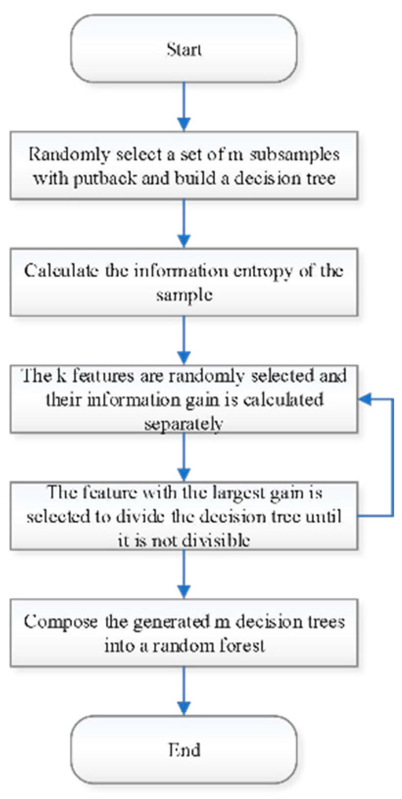
The algorithm flow of the random forest is shown in Figure 1.

The principle of Random Forest is shown in Figure 2.

1.1.3. Parameterization

1): n_estimators

n_estimators: this parameter controls the number of trees in the random forest. Theoretically, the more trees the better, but as the number of trees increases, the memory and time overheads will also increase. At the same time, the marginal benefits will diminish, meaning that the performance gain from each additional tree will become progressively smaller. Therefore, an appropriate number of trees needs to be chosen within an acceptable memory and time range.

2): random_state

random_state: this parameter is the random number seed, which is used to control the random pattern. In random forests, it affects the division pattern of the training and test sets. Setting the same random number seed ensures that the result of each division is the same.

3): Max_features

Max_features: This parameter controls the maximum number of features that can be used for splitting when building a decision tree. Smaller Max_features will result in larger differences between trees in a random forest, but if it is too small (e.g., 1), it may not be possible to select features when dividing nodes. log2”, etc. By default, the default value of Max_features is “auto”.

4): Min_samples_lesf

Min_samples_lesf: this parameter indicates the minimum number of samples allowed in a leaf node. If the number of samples in a leaf node is lower than Min_samples_lesf, a pruning operation may be performed to retain the parent node.

5): Min_samples_split

Min_samples_split: this parameter is the minimum number of samples required to split the internal nodes. If it is an integer, it is regarded as the minimum value; if it is a floating point number, it is regarded as a fraction, and the minimum number of samples required for each split is ceil (Min_samples_split * n_samples). The default value is 2.

In this paper, the settings of each parameter are shown in Table 1.

1.2. Predictive Modeling Based on Random Forest Algorithm

This paper constructed a random forest model by taking “whether to complete the paper with the help of AI” as the model output and different features as the model input. The ratio of the training set to the test set is 8:2.

In order to quantify the prediction effect of the model, the following indicators are set to evaluate the prediction results:

The accuracy rate indicates the proportion of samples judged as positive cases by the classifier that are actually positive cases. The calculation formula is as follows:

P r e c i s i o n = \frac{T r u e P o s i t i v e s}{T r u e P o s i t i v e s + F a l s e P o s i t i v e s}

(1)

True Positives are the number of samples that the model correctly predicts as positive and False Positives are the number of negative samples that the model incorrectly predicts as positive.

Recall is the proportion of samples that are actually positive that are determined to be positive by the classifier. The formula is as follows:

R e c a l l = \frac{T r u e P o s i t i v e s}{T r u e P o s i t i v e s + F a l s e N e g a t i v e s}

(2)

True Positives are the number of samples that the model correctly predicts as positive and False Negatives are the number of positive samples that the model incorrectly predicts as negative.

F1-score is the reconciled mean of precision and recall, which combines precision and recall. The formula is as follows:

F 1 - s c o r e = 2 \times \frac{P r e c i s i o n \times R e c a l l}{P r e c i s i o n + R e c a l l}

(3)

The value of F1-score ranges between 0 and 1, with higher values indicating better model performance.

Accuracy is the ratio of the number of samples correctly predicted by the model to the total number of samples. The formula is as follows:

A c c u r a c y = \frac{T r u e P o s i t i v e s + T r u e N e g a t i v e s}{T o t a l S a m p l e s}

(4)

Where True Positives are the number of samples that the model correctly predicted as positive examples and True Negatives is the number of samples that the model correctly predicted as negative examples.

The Macro Average is an arithmetic average of the metrics (e.g., precision, recall, F1-score, etc.) for each category. In multicategorical problems, it calculates the average of the metrics for each category, regardless of differences in the number of samples in the categories.

Weighted Average is a weighted average of the metrics for each category, where the weight of each category is determined by the proportion of the sample size of that category to the total sample size. This means that categories with larger sample sizes will have a greater impact when calculating the weighted average.

The predictions of the model are shown in Table 2.

By observing Table 2, it can be noticed that Random Forest can achieve 87% accuracy on this sample.

By creating a confusion matrix, it is possible to understand the effectiveness of the model’s predictions. The confusion matrix is a table used to evaluate the performance of a classification model and provides detailed information about the model’s performance in each category by comparing the predictions with the true labels. It helps us to calculate metrics such as accuracy, precision, recall, etc., to find out the types of errors in the model, and to adjust the classification thresholds to get more accurate predictions. The confusion matrix is an important tool for evaluating classification models, optimizing model performance and making decisions. As shown in Table 3.

As can be seen from Table 3, overall the model performs well in the three categories. Precision, recall, and F1- score are high for each category, indicating that the model strikes a good balance in predicting each category. The macro-averaging and weighted averaging metrics also reflect the overall performance, indicating that the model performs robustly in the different categories. Therefore, it can be said that the model performs appropriately on the categorization task “whether or not to complete a dissertation with the help of AI”.

1.3. Critical Feature Extraction and Performance Validation

In Section 2.2, all features are used as inputs to the model, which leads to a significant increase in training time. In order to reduce the training time, and to find out the important factors that affect students’ “whether to complete their thesis with the help of AI”, in this section, a few important features are extracted first, and then the extracted features are used as inputs to reconstruct the Random Forest prediction model. In this section, the extracted features are used as inputs to reconstruct the Random Forest Prediction Model, and to determine whether the prediction accuracy of the model changes significantly.

The extracted features are shown below:

1): If there is an AI learning tool, would you choose to use it?
2): Do you have any idea how to complete your assignments with the help of AI learning tools?
3): Do you have any idea how to complete quizzes with the help of AI learning tools?
4): What is your attitude towards the credibility of the AI learning tool in answering questions?
5): If you were to use an AI learning tool, what would you prefer to get out of it?
6): What safety aspects of using AI tools have you considered?

The above features are input into the random forest prediction model and the prediction performance is obtained as shown in Table 4.

From Table 4, it can be noticed that the model performs very balanced in each category. The precision, recall and F1-score for each category are between 0.82 and 0.88, which shows the robustness of the model in handling each category. The overall accuracy is 0.85, which means that the model also performs very well overall. In this case, the values of both “macro average” and “weighted average” are also very close to each other, which shows that each category has a similar influence on the overall assessment without any significant bias. In summary, the model still maintains a high prediction accuracy after reducing dozens of input features. This indicates that the extracted features can better reflect whether students “completed their dissertations with the help of AI”, and retain important features while eliminating redundant information.

The confusion matrix is also plotted as shown in Table 5.

Based on the confusion matrix and the calculated metrics, this model shows excellent performance in each category. Precision, recall, and F1-score are all quite high for each category, indicating that the model strikes a good balance in its predictions for each category. The macro-averaging and weighted averaging metrics also reflect the overall performance, indicating that the model performs very robustly in the different categories.

2. Classification of AI Usage Based on PCA-K-Means Algorithm

2.1. Feature Merging Based on the PCA Algorithm

In Section 2, this paper extracts several important factors affecting students’ “whether to complete the dissertation with the help of artificial intelligence”, and in order to further filter and merge the indicators, the features are downscaled based on the PCA algorithm in this section.

Mathematically, given a dataset X containing n samples and p features, the goal of PCA is to find a new set of uncorrelated variables, called principal components, to replace the original correlated variables. These principal components are obtained by linearly transforming the original data and are ranked in order of importance in order to retain as much information as possible while reducing the dimensionality of the data.

Take two-dimensional space as an example. Let the number of samples be 50, each sample contains x1 and x2 variables, and the two-dimensional plane is determined by x1 and x2. When the distribution direction of the sample data is not the x1 and x2 axes, but its distribution trend has a certain regularity, so consider that there may be some connection between the two, you can replace x1 and x2 with other variables, but if you replace them with any of these dimensions, it will surely result in the loss of the original data information. Therefore, the coordinate system is rotated counterclockwise by a certain angle Θ, so that the direction of the sample points with the greatest degree of dispersion is the z1 axis, and its orthogonal direction is the z2 axis.

The z1 and z2 rotation formula is:

\{\begin{matrix} z_{1} = x_{1} \cos Θ + x_{2} \sin Θ \\ z_{2} = {- x}_{1} \sin Θ + x_{2} \cos Θ \end{matrix}

(5)

The matrix is of the form.

(\begin{matrix} z_{1} \\ z_{2} \end{matrix}) = (\begin{matrix} \cos Θ & \sin Θ \\ - \sin Θ & \cos Θ \end{matrix}) (\begin{matrix} x_{1} \\ x_{2} \end{matrix}) = P^{T} x

(6)

where PT is an orthogonal matrix.

Calculate the mean vector of the data:

μ = \frac{1}{n} \cdot \sum_{i = 1}^{n} x_{i}

(7)

Calculate the covariance matrix:

C = \frac{1}{n} \cdot \sum_{i = 1}^{n} (x_{i} - \cdot \cdot μ) {(x_{i} - μ)}^{T}

(8)

Compute the eigenvalues and eigenvectors of the covariance matrix:

{C V}_{V} = λ \cdot λ V

(9)

Selection of principal components: This step involves selecting the eigenvectors corresponding to the largest K eigenvalues. These eigenvectors form a new space into which the original data is projected in this paper for the purpose of dimensionality reduction.

Projection into the new space:

y = vT (x − µ)

(10)

where y is the sample after dimensionality reduction and vT is the transpose of the matrix consisting of the eigenvectors. PCA is essentially the process of calculating feature vectors.

In this paper, the principal component of PCA is set to 3, because the original dimension is large, so we prevent losing too much information, and reduce it to 3 dimensions.

The calculated values by PCA are shown in Table 6.

2.2. Usage Classification Based on the K-Means Algorithm

By introducing K-means clustering, students can be categorized into multiple categories using self-supervised learning, and by looking at what these students have in common, it is possible to understand their attitudes toward AI learning tools and whether there is a potential risk of AI misuse.

The K-means clustering algorithm is for a given sample data and each

X = {X_{1}, X_{2}, X_{3}, \dots X_{n}}

is an m- dimensional vector (m-dimensional vectors consist of m features of the sample data), if the number of classification groups is k, the sample dataset X will be divided into k subsets

S = {S_{1}, S_{2}, \dots S_{k}}

each subset is a class and must satisfy the following conditions:

(1): Each data $X_{i}$ can be classified into only one class;
(2): Each class contains at least one data.

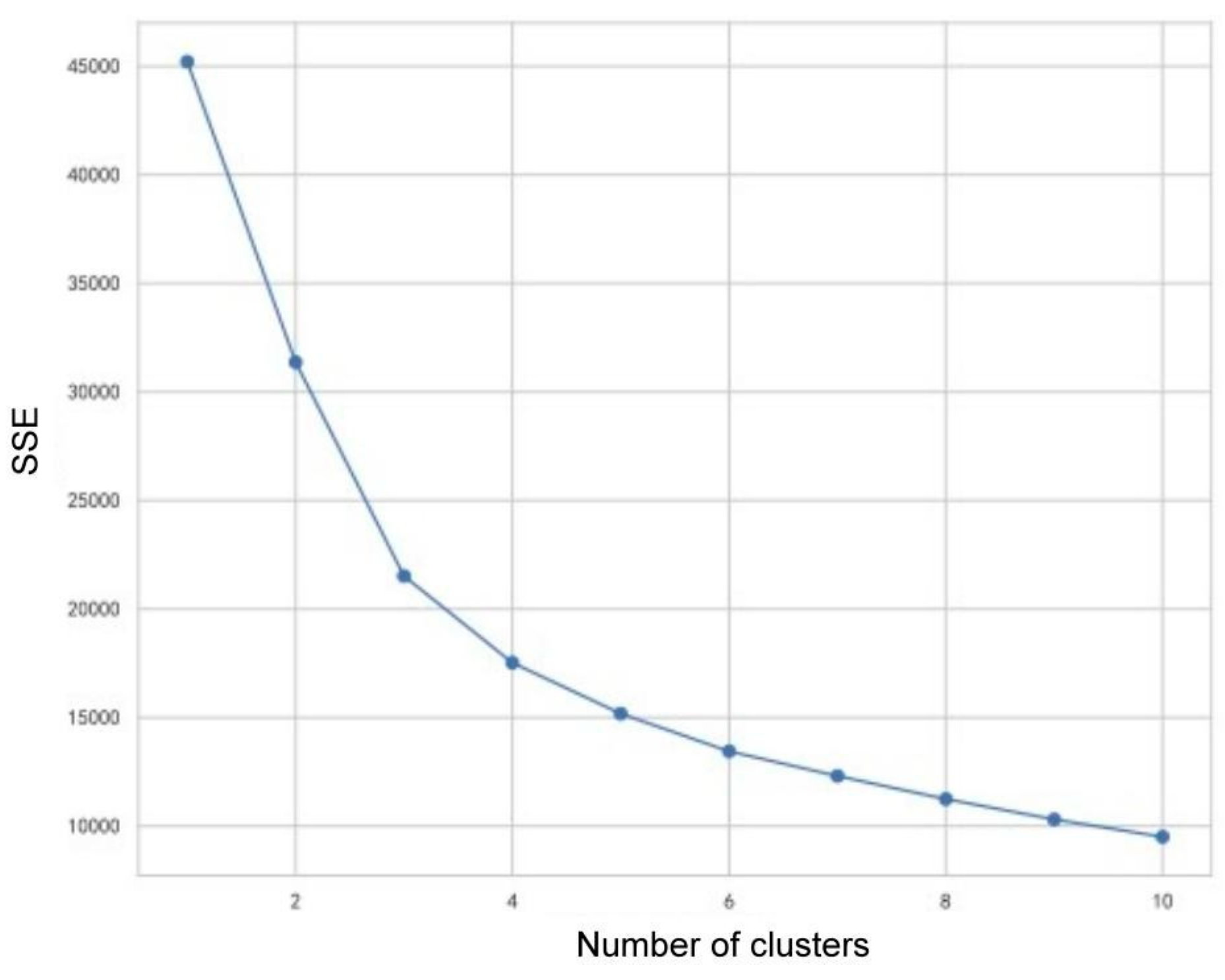
Although the Elbow Method does not have a clear mathematical formula, its core idea is to select the optimal number of clusters based on the relationship between SSE and the number of clusters. As the number of clusters increases, the SSE decreases, but at a slower rate. The number of clusters at the “inflection point” is considered to be a reasonable balance between fitting the data well and not introducing too many necessary clusters.

The relationship between K and SSE was generated and plotted on the Elbow Method as shown in Figure 3.

By using Calculate Silhouette Coefficient, we are able to draw its line graph, and the formula for Calculate Silhouette Coefficient is shown below:

(1): For each sample point i, calculate a(i), which is the average distance between point i and all other points in the same cluster. This can be expressed by the following formula:

$a (i) = \frac{1}{|C_{i}| - 1} \cdot \sum_{j \in C_{i, j} \neq i}^{} d (i, j)$

(11)

where $C_{i}$ is the cluster containing sample point i, $C_{i}$ distance between sample points Ci and d(i,j) is the distance between sample points i and j.
(2): For each sample point i, calculate b(i), which is the minimum average distance between point i and all other points not in the same cluster. This can be expressed by the following formula:

$b (i) = \min_{k \neq i} \frac{1}{|C_{k}|} \sum_{j \in C_{k}}^{} d (i, j)$

(12)

where $C_{k}$ is an arbitrary cluster that does not contain sample point i.
(3): For each sample point i, the profile coefficient s(i) is:

$s (i) = \frac{b (i) - a (i)}{m a x {a (i), b (i)}}$

(13)

Define s(i) = 0 if sample i is the only member of the cluster it is in (i.e., | $C_{i}$ | = 1).
(4): The average of the profile coefficients of all sample points is the profile coefficient of the entire data set:

$S = \frac{\frac{1}{π}}{N} \sum_{i = 1}^{N} s (i)$

(14)

Where N is the total number of samples in the data set.

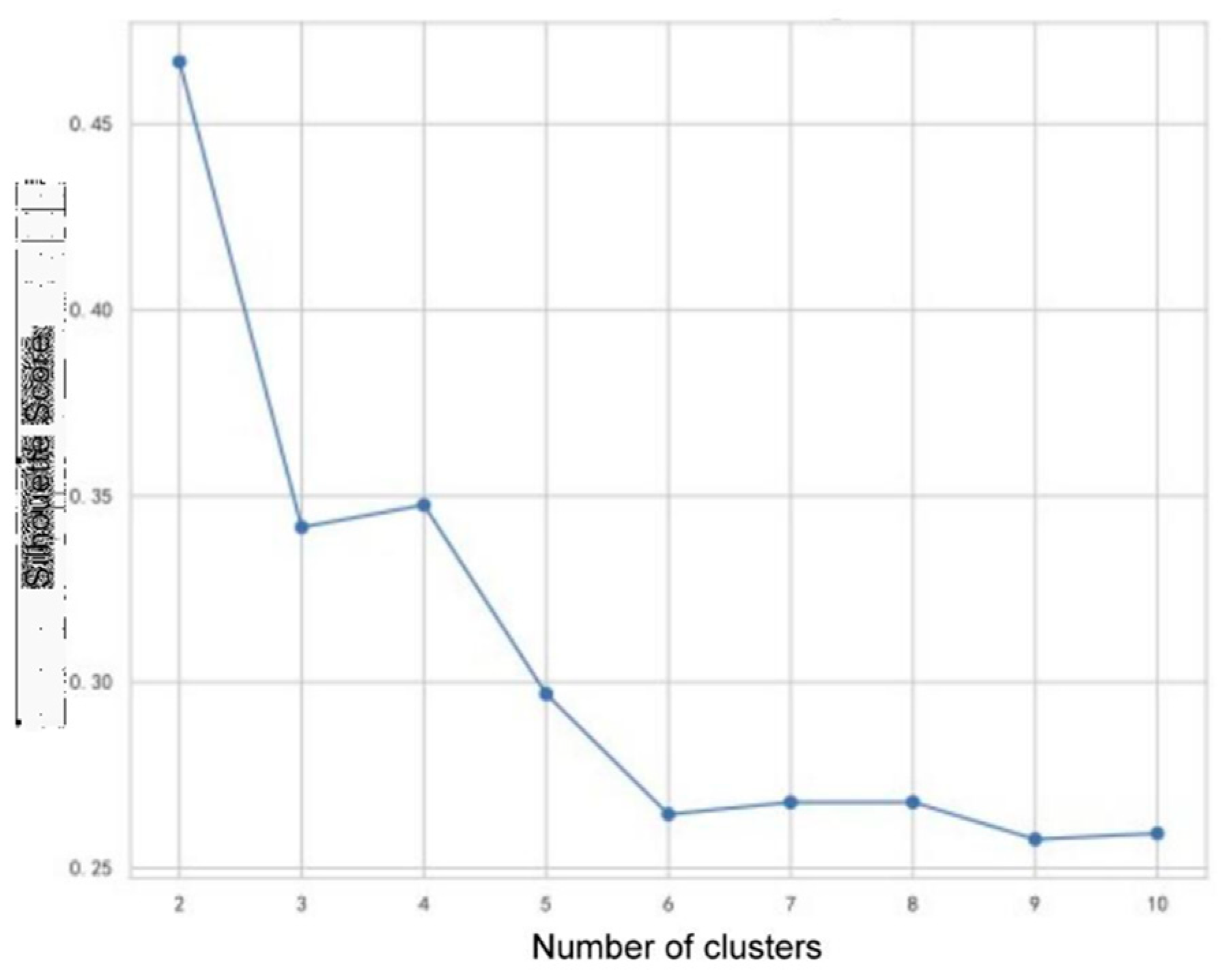
The line graph of the Silhouette Coefficient is shown in Figure 4. In the Elbow Method graph, the curve is relatively smooth, the inflection point is not obvious, and there is a small inflection point at K=3, while in the Silhouette Coefficient graph, the Silhouette Coefficient varies greatly between K=2 and K=3, and the clustering will mainly divide students into two categories of “optimistic about AI” and “not optimistic about AI”. In the Silhouette Coefficient plot, when K=2 and K=3, the Silhouette Coefficient is quite different, and the clustering classifies the students into two categories: “favorable to AI” and “unfavorable to AI”, and when K=3, the clustering classifies the students into “favorable to AI”, “neutral”, “unfavorable to AI” and “neutral”. “For this reason, we chose K=2 because it is more directly responsive to the results and is more interpretable for our subsequent visualizations, and because K=2 has a higher Silhouette Coefficient than K=2. Silhouette Coefficient.

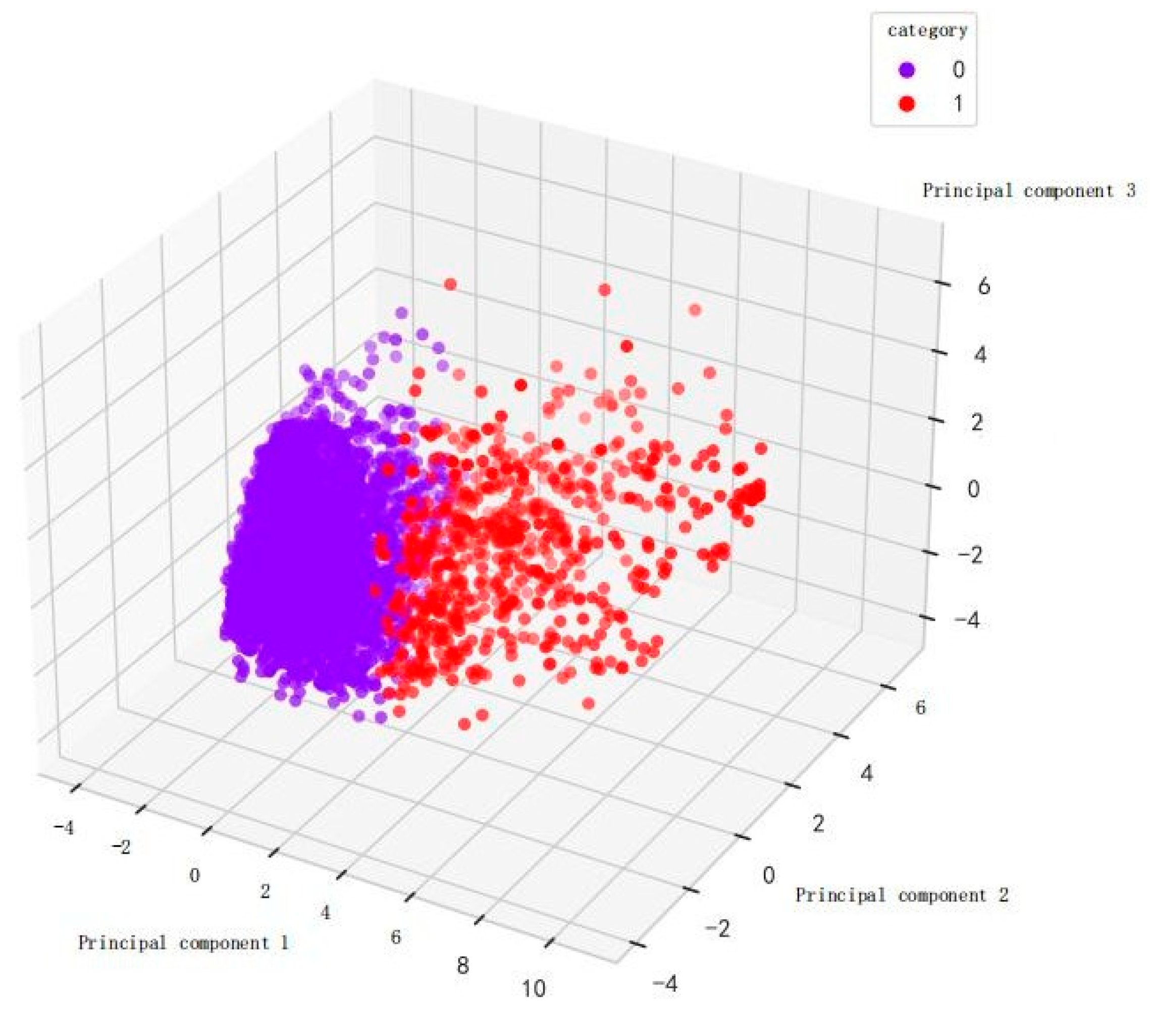
The clustering results are visualized as shown in Figure 5.

Through the analysis of this paper, it can be learned that most of the students are willing to accept such a new thing as AI for learning, and most of them think that they can improve themselves through AI, which means that this part of the students want to use AI to get higher; while there are a small number of students who want to use AI to cope with the homework and exams, and they want to get something for nothing, letting AI replace the process of their own thinking; and last but not least, there is a small part of students who are more resistant to AI and unwilling to contact such technology, which may be due to a number of factors, such as Finally, there is a small number of students who are more resistant to AI and are not willing to contact such technology, which may be due to a variety of factors, such as the fear of information leakage, the correctness of AI and other issues.

3. Conclusion

The findings of this study shed light on the multifaceted relationship between students and AI technology. The results from the random forest model and PCA-K-means algorithm demonstrate that while the majority of students embrace AI to enhance their capabilities, a subset of students may resort to AI primarily for exam- related tasks. Understanding these nuances is crucial for educators and policymakers as they navigate the integration of AI in educational settings, ensuring that AI is leveraged to enrich learning experiences and foster genuine skill development among students. After analyzing this paper, it is evident that the majority of students are open to embracing AI for learning, believing that it can enhance their educational experience. They see AI as a tool for self-improvement, aiming to leverage it for academic advancement. However, a minority view AI as a means to bypass the cognitive effort involved in homework and exams, seeking effortless gains. Additionally, a small faction of students exhibit resistance to AI, possibly influenced by concerns such as data security, AI accuracy, and other related apprehensions.

References

Thomas K. F. Chiu, Qi Xia, Xinyan Zhou, Ching Sing Chai, and Miaoting Cheng. 2023. Systematic literature review on opportunities, challenges, and future research recommendations of artificial intelligence in education. Computers and Education: Artificial Intelligence 4, (January 2023), 100118. [CrossRef]
Chunling Geng. 2024. Research on the effectiveness of interactive e-learning mode based on artificial intelligence in English learning. Entertainment Computing 51, (September 2024), 100735. [CrossRef]
Sabrina Habib, Thomas Vogel, Xiao Anli, and Evelyn Thorne. 2024. How does generative artificial intelligence impact student creativity? Journal of Creativity 34, 1 (April 2024), 100072. [CrossRef]
Manuela-Andreea Petrescu, Emilia-Loredana Pop, and Tudor- Dan Mihoc. 2023. Students’ interest in knowledge acquisition in Artificial Intelligence. Procedia Computer Science 225, (January 2023), 1028–1036. [CrossRef]
Wilson Kia Onn Wong. 2024. The sudden disruptive rise of generative artificial intelligence? An evaluation of their impact on higher education and the global workplace. Journal of Open Innovation: Technology, Market, and Complexity 10, 2 (June 2024), 100278. [CrossRef]
Zhou, P., Peng, R., Xu, M., Wu, V., Navarro-Alarcon, D. 2021. Path planning with automatic seam extraction over point cloud models for robotic arc welding. IEEE robotics and automation letters, 6(3),(April 2021), 5002-5009. [CrossRef]
Jinxin Xu, Haixin Wu, Yu Cheng, Liyang Wang, Xin Yang, Xintong Fu, and Yuelong Su. 2024. Optimization of Worker Scheduling at Logistics Depots Using Genetic Algorithms and Simulated Annealing. arXiv:cs.NE/2405.11729 [cs.NE]. (May 2024). [CrossRef]

Figure 1. Random Forest Algorithm Flow.

Figure 2. Random Forest Principle.

Figure 3. Elbow Diagram.

Figure 4. Silhouette coefficient.

Figure 5. Clustering results.

Table 1. Random Forest Parameter Settings.

parameter	value
n_estimators	700
random_state	42
Max_features	Auto
Min_samples_lesf	1
Min_samples_split	2

Table 2. Random Forest Model Prediction Performance.

	precision	recall	f1-score	support
1.0	0.85	0.87	0.86	290
2.0	0.86	0.86	0.86	346
3.0	0.90	0.87	0.89	272
accuracy	/	/	0.87	908
macro avg	0.87	0.87	0.87	908
weighted avg	0.87	0.87	0.87	908

Table 3. Confusion matrix.

	Predicted Labels
True Labels	250	32	6
	28	300	20
	17	18	240

Table 4. Predicting performance.

	precision	recall	f1-score	support
1.0	0.82	0.85	0.84	290
2.0	0.86	0.84	0.85	346
3.0	0.88	0.87	0.87	272
accuracy	/	/	0.85	908
macro avg	0.85	0.85	0.85	908
weighted avg	0.85	0.85	0.85	908

Table 5. Confusion matrix.

Predicted Labels
	2500	31	12
True Labels	35	290	20
	19	17	240

Table 6. Calculated values by PCA.

	0	1	2
0	-3.549843	2.509355	-0.158039
1	3.060733	-2.079833	2.650664
2	-2.514655	-0.044689	0.844996
3	-1.489571	-0.883850	0.359377
4	-1.204717	1.390635	0.790669

Disclaimer/Publisher’s Note: The statements, opinions and data contained in all publications are solely those of the individual author(s) and contributor(s) and not of MDPI and/or the editor(s). MDPI and/or the editor(s) disclaim responsibility for any injury to people or property resulting from any ideas, methods, instructions or products referred to in the content.

© 2024 by the authors. Licensee MDPI, Basel, Switzerland. This article is an open access article distributed under the terms and conditions of the Creative Commons Attribution (CC BY) license (http://creativecommons.org/licenses/by/4.0/).

Copyright: This open access article is published under a Creative Commons CC BY 4.0 license, which permit the free download, distribution, and reuse, provided that the author and preprint are cited in any reuse.

MDPI Initiatives

Important Links

Choose an area of interest and we will send you notifications of new preprints at your preferred frequency.

Disclaimer

Research on Students’ Utilization of Artificial Intelligence Based on Random Forest Model and PCA-K-means Algorithm

Abstract

1. Introduction

1.1. Random Forest Algorithm

1.1.1. Decision Tree

1.1.2. Ideas for the Construction of a Random Forest Algorithm

1.1.3. Parameterization

1.2. Predictive Modeling Based on Random Forest Algorithm

1.3. Critical Feature Extraction and Performance Validation

2. Classification of AI Usage Based on PCA-K-Means Algorithm

2.1. Feature Merging Based on the PCA Algorithm

2.2. Usage Classification Based on the K-Means Algorithm

3. Conclusion

References

MDPI Initiatives

Important Links

Subscribe