1. Introduction
Exploration of the ocean is vital for harnessing its abundant resources [
1]. Underwater robots are crucial instruments to explore the ocean, which enables image-based target detection tasks. Due to light attenuation and scattering in seawater, the quality of these images is often compromised. Consequently, underwater image enhancement algorithms are critical in correcting these distortions [
2] (
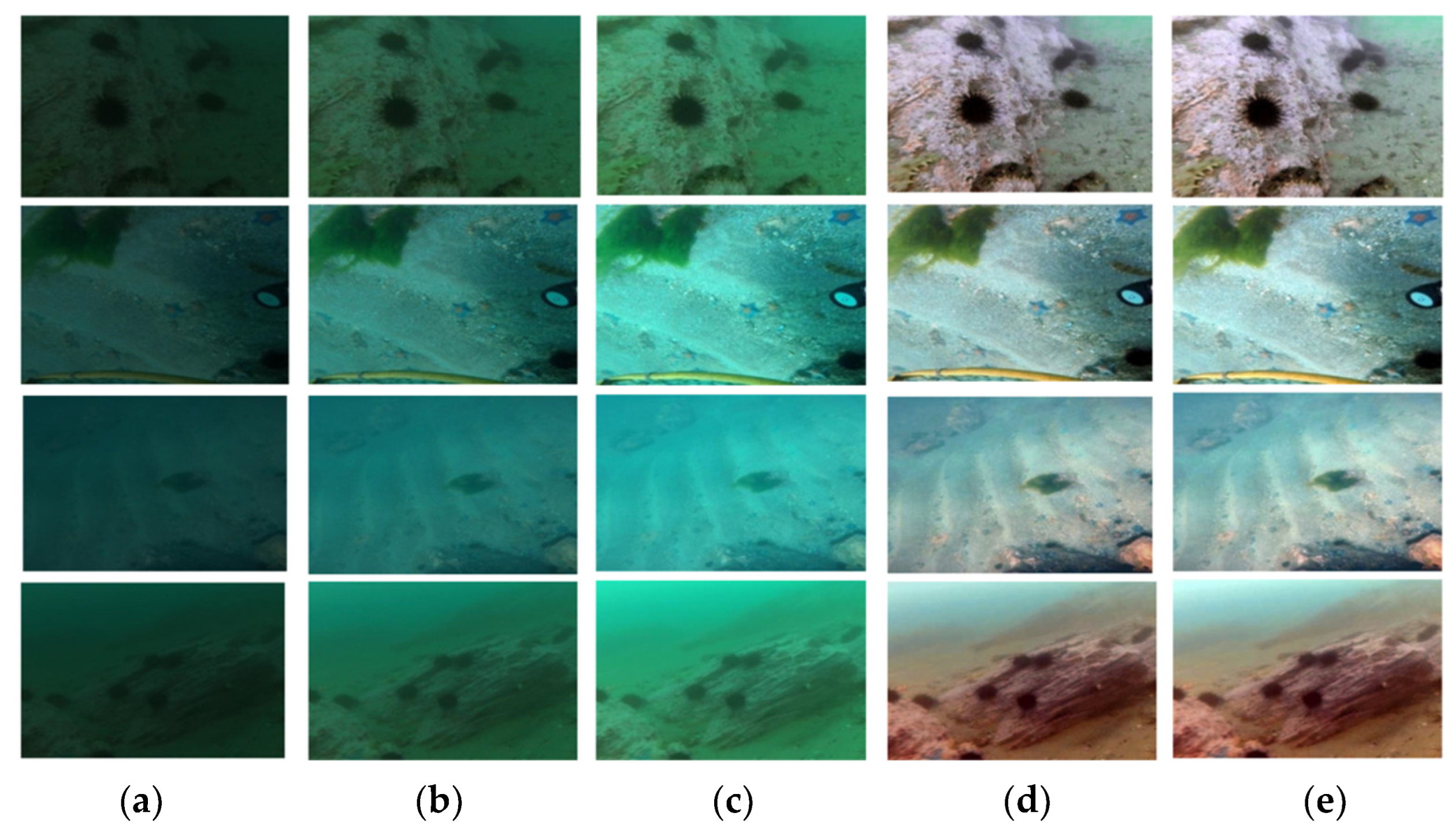
Figure 1), establishing a significant research area within the fields of computer vision and underwater robotics. Four methods [
3] are selected to test the same image with our computer, showcasing different repaired quality. Therefore, underwater image processing faces significant challenges due to color distortion and reduced contrast caused by the absorption and scattering effects of water.
Underwater Research in image enhancement focuses on improving the quality of distorted underwater images, with a focus on restoring color distortion information [
4]. Some scholars have explored non-deep learning approaches and have made some progress. Non-deep learning methods rely on statistical assumptions and model to enhance underwater images, such as Underwater Dark Channel Prior (UDCP) [
5], Image Blur Recovery [
6], and Underwater Light Attenuation Prior (ULAP) [
7]. Cheng et al. [
8] pointed out that the dissolved substances in water can weaken the imaging process, and influence the attenuation parameters of light propagation in water. Drews et al. proposed an underwater prior method by utilizing red channel information [
9]. Li et al. proposed an underwater light attenuation prior (ULAP) model to restore image quality [
10]. Ma et al. devised a wavelet transform network that decomposes input images into frequency maps to enhance image details [
11]. However, the complexity of underwater environments often leads to inaccuracies in parameter estimation for these methods.
Currently, neural networks have been widely employed to various visual tasks [
12]. In contrast, extensive datasets and specialized loss functions have been utilized by deep learning techniques to train deep neural networks for image quality enhancement, including models like Underwater Residual Network (UResNet), Shallow Underwater Network (UWNet), and Underwater Convolutional Neural Network (UWCNN) [
13]. Mean square error loss and edge difference loss are used to optimize convolutional neural networks for image enhancement [
14]. By employing conventional convolutions, Naik et al. developed a network specifically for underwater image enhancement, which demonstrates effective enhancement capabilities on public datasets [
15]. Li et al. introduced a residual network-based underwater image enhancement algorithm [
16]. Chen et al. introduced an end-to-end neural network enhancement model that integrates residual structures and attention mechanisms [
17]. Current enhancement algorithms predominantly rely on convolutional neural networks, but they often utilize a single feature extraction backbone. However, the features extracted from these models are often insufficiently detailed.
Wang et al. utilized Generative Adversarial Networks (GANs) to design a feature enhancement network [
18,
19]. Moreover, the underwater generative adversarial net-works (UGANs) [
20] scheme has been established for UIE task by using encoder–decoder structure [
21,
22], whereby the preservation of rich semantic information can be achieved. Junjun Wu et al. have developed a multi-scale fusion generative adversarial network named Fusion Water-GAN (FW-GAN), which aims to improve underwater image quality while effectively preserving rich semantic information. This network integrates four convolutional branches to achieve this goal [
23]. Kei et al. created a dataset that includes both image and sonar data specifically designed for low-light underwater environments, utilizing a Generative Adversarial Network (GAN) to improve image quality. Experimental results show that this method achieves better detection performance [
24]. Zhang et al. collected images from different angles and then calculated the camera poses for each angle. They fed the collected image sequences and their corresponding poses into a Neural Radiance Field (NeRF), synthesizing new viewpoints and improving the effect of 3D image reconstruction [
25]. Adversarial learning methods are mostly based on object detection with similar quality or visibility, and acquiring clear sample data for these models remains a formidable task.
Deep learning encompasses various backbone architectures, including the widely utilized Convolutional Neural Networks (CNNs) and Transformers [
26,
27], which has gained popularity in computer vision tasks. The Transformer architecture incorporates features like multi-head mechanisms and multi-layer perceptions, making it versatile for a range of visual tasks [
28]. Zamir et al. [
29] employed an encoder-decoder structure to obtain features at different scales, achieving image enhancement in rainy and foggy weather conditions. Song et al. modified attention modules within the network layers, constructing a parameter-adjustable dehazing network [
30]. Although the Transformer architecture shows great potentiality for computer vision tasks, its high computational complexity often results in increased computational load and longer processing times.
Despite advancements in current methods for addressing underwater image distortions, challenges persist in achieving high-quality restoration. To produce high-quality images, our research try to overcome the uncertainty in generated images by utilizing the complementary features of different neural network frameworks. This paper introduces a new model for enhancing the quality of underwater images, aiming to tackle issues such as color shifts, unrealistic colors, and reduced contrast [
31]. Furthermore, a matrix linear computation approach has been designed to minimize the computational delays caused by network stacking. To this point, an innovative approach is proposed to extract both local and global image features. This network integrates visual Transformer models with CNN networks to enhance the overall restoration process. Additionally, information fusion weights are calculated from the Fourier transform features of original image. The main advantage of our work are as followed:
1) A novel Transformer model that extracts local features has been proposed. It incorporates PSNR attention and linear operations to significantly reduce computational load and alleviate color artifacts.
2) Additionally, a novel global feature extraction network is devised, which leverages both temporal and frequency domain characters to enrich image features.
3). Additionally, a feature fusion method, utilizing the Fourier transform of the original image, has been introduced to optimize global feature weights through high-frequency Fourier transforms and local feature weights via low-frequency Fourier transforms.
2. Materials and Methods
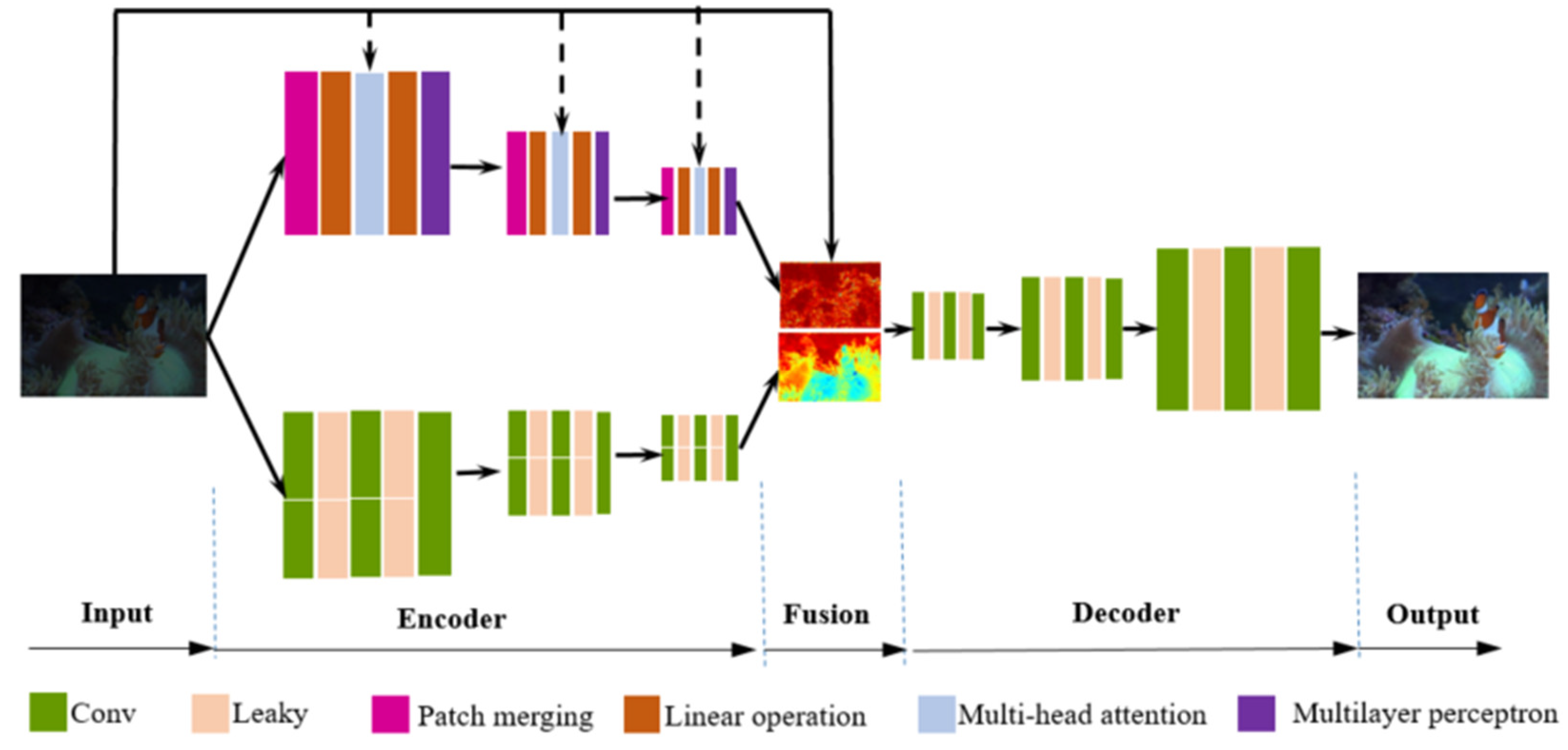
Figure 2 depicts our detection framework. This network incorporates both CNN and Transformer backbones, which is designed to extract both global and local features, respectively. These extracted features are fused at the smallest down-sampling size. Additionally, the low-frequency and high-frequency information of the original image is obtained via Fourier transform, serving as fusion weights for the extracted CNN and Transformer features.
2.1. Two branches’ Feature Extraction Network
Conventional low-light image enhancement networks typically employ convolutional structures within the feature layers, predominantly extracting image information from the image’s bright regions. These regions are rich in visible content or signals. However, in some non-prominent regions, fine-grained features may be lost, leading to a decrease in detection accuracy.
To this point, we employ two backbones for image enhancement. Information from both global and local regions complements each other, and this differentiation can be determined based on the distribution of Fourier transforms on the image. On one hand, for image regions characterized by high-frequency Fourier transforms, their features predominantly manifest in the globally salient information. On the other hand, in image regions corresponding to low-frequency Fourier transforms, the Transformer predominantly captures local detailed information. This methodology facilitates the extraction of diverse image features.
As to the encoder framework, we devised two different backbones for feature extraction. One employs transformers, while the other utilizes convolutional structures. Each backbone incorporates a top-down feature pyramid extraction network, segmented into three levels. The input dimension of the first layer features is 6 dimensions, yielding 64 dimensions as output. Both the second and third levels’ feature extraction operations utilize 64 channels.
CNNs excel at extracting edges, textures, and simple shapes from images. Transformers, on the other hand, excel at identifying long-range dependencies and inferring local information. By integrating the local features extracted by Transformers with the global textures identified by CNNs, we can produce richer and more diverse representations. This combined approach is more effective at handling noise and variations in data. Moreover, hybrid models can better adapt to different types of data, which can deal with spatial and sequential information simultaneously. Thereby, the method can enhances the model’s recognition and classification capabilities.
2.2. Implementation of the CNN Branch
Convolutional Neural Networks (CNNs) is a types of deep learning model specifically designed to process image data. CNNs employ convolutional layers for extracting local features, pooling layers to diminish data dimensionality and computational complexity, and fully connected layers for classification. The core advantages of CNNs lie in their local connections and shared weight, which make them particularly effective for image recognition and classification tasks.
Convolutional Neural Networks extract features by sliding convolutional kernels over the pixels’ matrix of the input image, computing the weighted sum of local regions to generate feature maps (
Figure 3 (b)). The kernels capture local features like edges and textures. Subsequently, activation functions perform nonlinear mappings on these features, enhancing the model’s ability to filter key characteristics. The parameters of the network are optimized through the error back propagation and iterative learning. This learning process automatically constrains the input and maximizes the activation of the output.
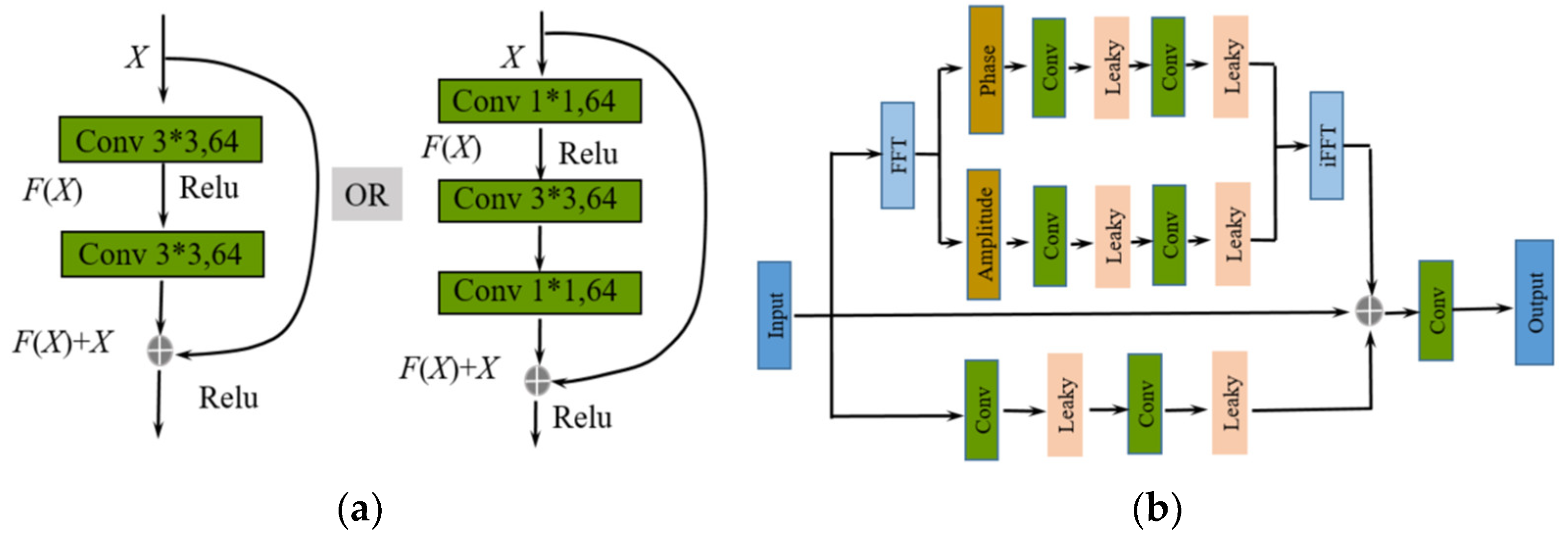
Residual Network (ResNet) is an improved version of CNNs, introducing skip connections or residual connections (
Figure 4 (a)). These connections allow gradients to pass directly from later layers to earlier layers, addressing the issues of vanishing and exploding gradients in training deep networks. By stacking more layers, ResNet achieves deeper network architectures than the traditional CNNs, and have demonstrated significant performance in various visual tasks [
33].
Different from the ResNet network, some researchers have noted that the brightness degradation on images primarily resides in the magnitude components of Fourier transformation, while the rest exists in the phase components [
34]. Inspired by previous research on Fourier transformation, this backbone further introduces the correlation properties between magnitude component and brightness to enhance feature extraction effectiveness. In this backbone, we designed two stages’ feature architecture (
Figure 4 (b)). In stage one, brightness of low-light image features is enhanced by optimizing the amplitude in Fourier space. In stage two, features from convolutional neural networks are further integrated.
In stage one, given an input image
x with a dimensions of
H×W, its transformation into the frequency space is represented by Equation (1):
Where, ℎ and w denote coordinates in the temporal domain, while
u and
v represent coordinates in the frequency domain. To extract the amplitude and phase components, the Fourier processing (FFT) block extracts frequency features (
Figure 4). Subsequently, two 1x1 convolutional layers with Leaky activation are applied to each branch. Finally, an inverse Fourier transform (iFFT) is applied to convert these two branches back to the spatial domain.
The Fourier transformation primarily relies on convolutional changes in the frequency domain to enhance brightness, while lacking convolution operations in the temporal domain for extracting details. Therefore, in the second stage, convolution operations in the temporal domain are employed to enrich features. Finally, to achieve the ultimate feature fusion, dimension addition and reduction operations are separately applied to the features in the temporal-frequency domain.
Compared with the commonly used residual network (
Figure 4 (a)), our method with the Fourier Transform(
Figure 4 (b)) can convert convolution operations into multiplication operations in the frequency domain, thereby enhancing the efficiency of convolution calculations. By enhancing specific frequency components, specific edge features can be accentuated, which is especially useful for image enhancement. However, during the inverse Fourier Transform process, some important information may be lost. Therefore, integrating features from the temporal domain is crucial to preserve specific characteristics.
2.3. Implementation of the Transformer Branch
Unlike CNNs, which extract features through global attentions, transformers capture local features from token regions. Local feature extraction is achieved through the matrixes’ multiplication, which has been validated in various high-level and low-level tasks. Assuming the feature dimensions are
h*w*C and the token size is
p*p, the total number of feature tokens can be calculated as
m=(
h/p)* (
w/p)*
C. Moreover, multi-head self-attention (MSA) modules and multi-layer perceptions (MLP) are employed in transformer. Assuming the input features to the transformer have the same dimensions, tokens are merged into a sequence of features with multiple heads (
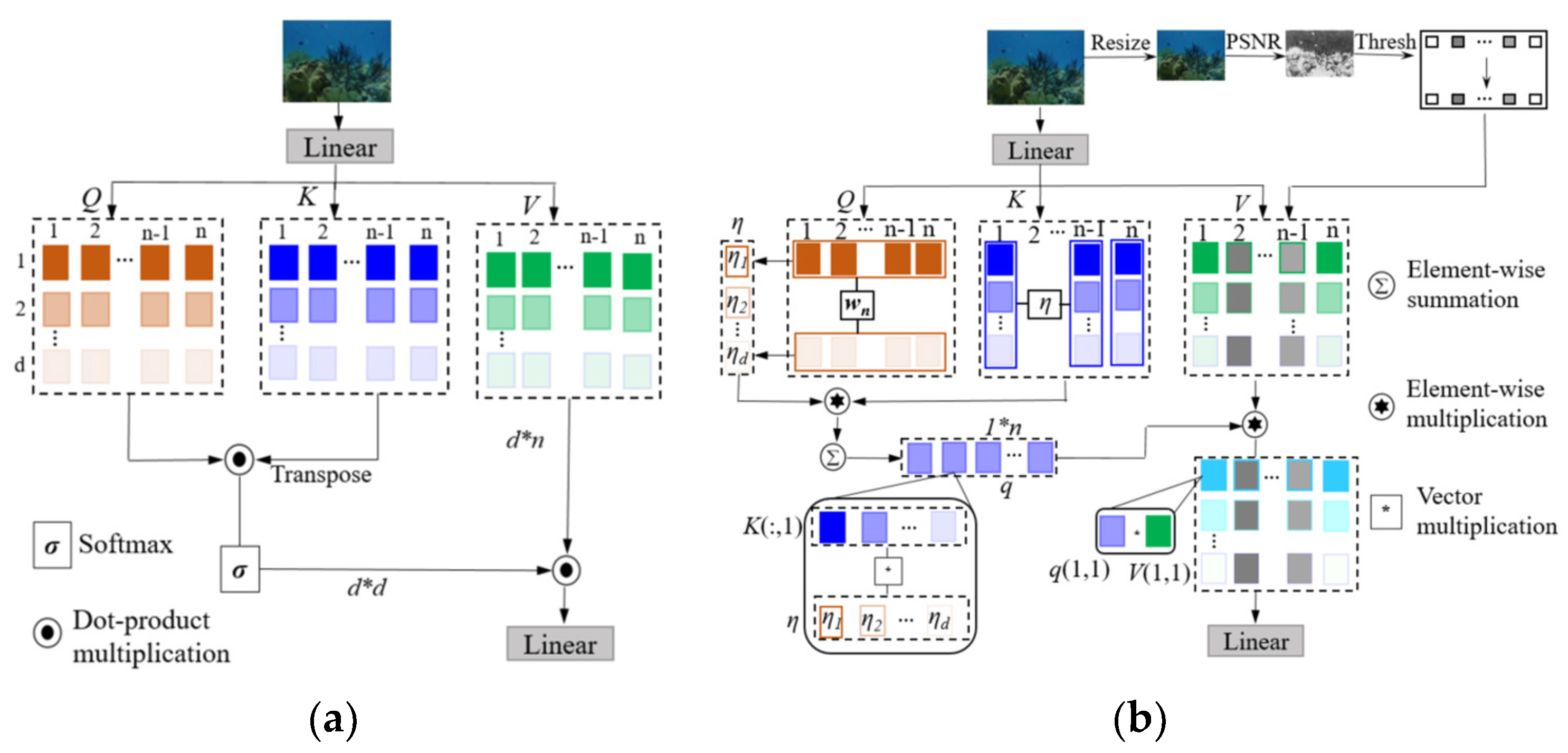
Figure 5 (a)).
Q*
KT=(
Rd*n)*(
Rd*n)
T= R
d*d, and its computation load=
d2*
n. Then, (
Rd*d)*(
Rd*n) =
Rd*n, and its computation load=
d2*
n. In summary, the total computation load= 2
d2*
n. The calculation process of feature transformation and computational complexity are respectively depicted in Equation (2): and Equation (3):
Where, Q is the query matrix, Q is the key matrix, and Q is the value matrix.
To alleviate calculation complexity, the method in
Figure 5 (b) replaces traditional dot-product multiplication with element-wise multiplication. Typically,
Q,
K, and
V each have dimensions of
Rd×n. To compute the attention weights for extracting features from underwater images, the query matrix is initially multiplied by a trainable parameter vector (
wn ∈
Rn). This process results in the generation of a global attention vector of size
ηd in Equation (4):
Next, the
K matrix undergoes element-wise multiplication with the global attention vector
ηd to yield the global query vector
q. As shown in
Figure 5.(b),
q∈
R1*n. Subsequently, this global vector
q is element-wise multiplied with the
V matrix to generate global features that merge information from both the
Q-matrix and
K-matrix. Unlike previous dot-product computations, the computational load of element-wise multiplication is linearly related to the parameters (
d*n), alleviating overall computational load. Following this, we perform another transformation to activate the final information in Equation (5):
Where
T denotes the activation operation. To mitigate the influence of extremely dark regions on inference, SNR map is utilize to guide the learning attention of the transformer. For an input image
I∈RH x W x 3, with its corresponding SNR map
S∈
RH x W,
S is adjusted into
S’∈Rh x w to align with the dimensions of the feature map
F. Then,
S’ is partitioned into
m patches, and the average value for each patch is calculated.
Si ∈[0,1], where
i={
1,..., m}. This masking mechanism effectively prevents the influence of features with very low signal-to-noise ratio (SNR), as illustrated in
Figure 5(b). The the
i-th mask value of
S’ is designed in Equation (6):
The masking calculation process for the
x parameter is expressed in Equation (7):
As shown in
Table 1, the total calculation load is 3
d*
n, which is far less than the previous calculation load 2*
d2*
n. According to the commonly used dot-product multiplication in
Figure 5 (a), the computational complexity of the self-attention mechanism scales quadratically with the sequence length (
d2), causing a significant increase in resource consumption when the sequence length is large. Due to the large number of parameters in each layer, Transformer models are typically much larger than CNNs, requiring more memory and computational power for training and inference. By adopting the proposed hybridized block modular approach, the computational load can be reduced from 2
d2n to 3
dn, offering a substantial advantage. The integration of CNN and Transformer models increases complexity and computation time. Therefore, we reduce the algorithm’s complexity through matrixes’ element-wise multiplication.
It is worth noting that similar block or token attention has been developed. Zhou et al. divided large images into smaller blocks, utilizing a trained rCNN as a block descriptor for image forgery detection [
35]. Bei et al. introduced the block matching and grouping criterion, applying a convolutional neural network (CNN) within each block for 3D filtering to develop a well-suited denoising model [
36]. Abbas et al. created an innovative hybrid block-based neural network model, integrating expert modular structures and divide-and-conquer strategies with a genetic algorithm (GA) [
37]. To generate high-resolution landslide susceptibility maps, each sub-network module employs input blocks, layers of hidden blocks, and an additional decision block (
Figure 6 (a)). Different from the independent block’s method, the element-wise multiplication operation is developed in the research to extract the cross-attention (
Figure 6 (b)).
In order to compare the performance of different block based methods, the two structures in
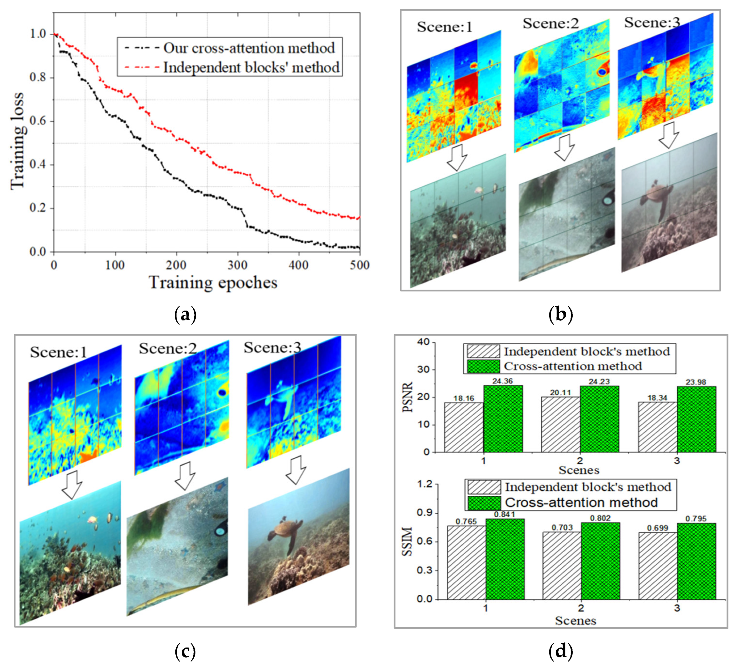
Figure 6 were used to train and enhance images, respectively. Images from three different scenarios are displayed. Despite the significant development and approved capability of image processing systems through the advanced block-based or modular structures, our presented model in this study offers three significant advantages. Firstly, it can reduce learning losses and accelerate model convergence (
Figure 7 (a)). Secondly, it captures global forward-backward attention more effectively, and extracts the continuous features, which reduces information loss caused by independent blocks (
Figure 7 (b) and (c)). Thirdly, it brings high-quality enhanced images with higher PSNR and SSIM indexes (
Figure 7 (d)).
2.4. Fusion Attention Based on High-Pass and Low-Pass Filters
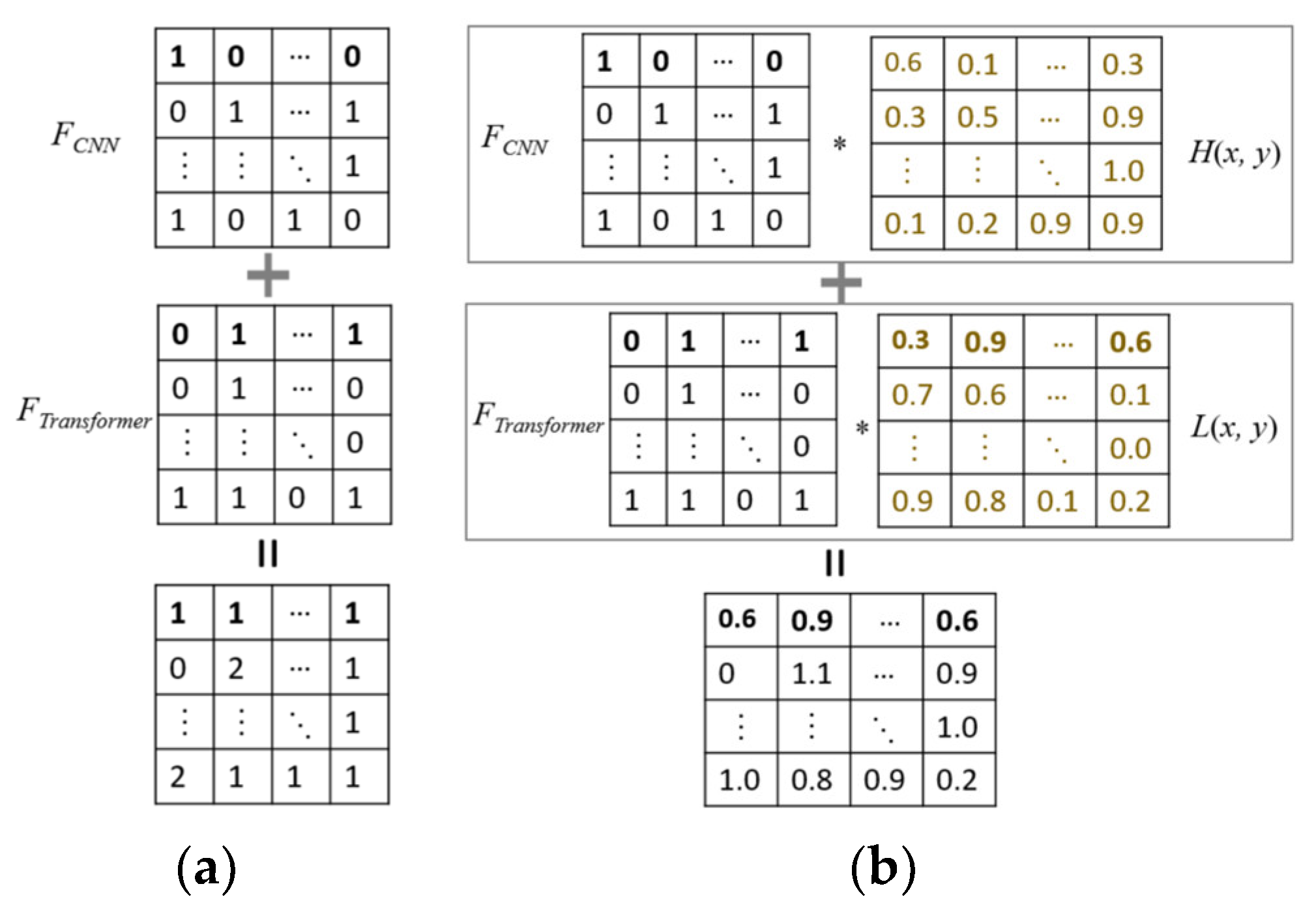
The torch.add method is commonly used to perform element-wise addition of tensors [
35]. This method checks the shapes of the input tensors. When the shapes are aligned, the addition operation is performed element by element. This means that corresponding elements from each tensor are added together, producing a new tensor as the result. The result of the addition operation can be stored into a new tensor. While this method can combine different features, it cannot differentiate or utilize the advantages of different features.
Different from the traditional torch.add method, the significant difference of low-frequency and high-frequency features is valuable and can be utilized. The display of an image relies on trigonometric frequency components. High-frequency signals cause rapid changes, leading to sharp edges within the image. Conversely, low-frequency signals induce more gradual changes, contributing to smoother appearance within the image. The role of filters is to pass or suppress certain frequency components of an image.
The Fourier transform serves as a bridge between the temporal domain and the frequency domain (
Figure 6). Ideal low-pass filtering, a method for image smoothing, retains low-frequency components. The transfer function of an ideal low-pass filter is represented in Equation (8):
Where
M and
N denote the length and height of the image, respectively.
D(
u, v) denotes the frequency domain of the image, and
f(
x, y) represents the temporal domain of image. The range of
u is [0,
M−1], and the range of
v is [0,
N−1].
D(
u, v) denotes the distance from the point (
u, v) in the frequency domain to the center, while
D0 denotes the cutoff frequency.
L(
u, v) denotes the low-pass filters in the frequency domain.
L(
x, y) denotes the low-pass results in the temporal domain.
Figure 9 illustrates the corresponding low-pass filter functions and their corresponding filtering outcomes.
Different from the low-pass filters, high pass filters enhance the details and edges of an image by removing low-frequency components. The basic principle is to set the low-frequency components in the frequency domain to zero and only retain the high-frequency components.
H(
u, v) denotes the high-pass filters in the frequency domain.
H(
x, y) denotes the high-pass results in the temporal domain.
Figure 10 illustrates the associated high-pass filter functions and their filtering results. The transfer function of a high-pass filter is represented in Equation (9):
We utilize Fourier transforms to calculate fusion weights for integrating different backbone features (
Figure 11 (b)). Low-frequency features are extracted by the Transformer to align with locally smooth features. Sharp edge details are captured by convolutional neural networks to match the high-frequency features. Both high and low-frequency features are normalized to the [0-1] range. The different fusion calculation is illustrated in Equation (10):
Low-frequency Fourier variations correspond to Transformer features, while high-frequency Fourier variations correspond to CNN features. Compared with the commonly used torch.add in
Figure 11 (a), the combination of CNNs and Transformers can fully leverage the different advantages. This method not only enhances feature representation capabilities and robustness, but also optimizes the use of computational resources.
3. Experimental Validation
3.1. Dataset and Experimental Designation
We evaluate the algorithm’s performance by using two publicly accessible datasets: LSUI [
36] (Large-Scale Underwater Image dataset) and UIEB dataset [
37]. LSUI comprises 5000 underwater images with varying exposure levels. The UIEB dataset includes pairs of low-exposure and high-exposure images, with 800 pairs designated for training, 150 pairs for validation, and 90 pairs for testing. The LSUI and UIEB datasets play crucial roles in underwater image enhancement research. LSUI, with its large and diverse data volume, offers ample material for training and testing deep learning models. Due to its high-quality annotated image pairs, UIEB is a key resource for evaluating and optimizing algorithms. By utilizing the two datasets, it provide us more powerful and robust underwater image enhancement algorithms, offering higher quality image processing solutions.
Our framework was implemented in PyTorch [
38], and the training and testing processes are conducted on a computer equipped with a 2080Ti GPU. Gaussian distribution was used to randomly initialize the network training parameters. And standard data augmentation techniques, such as vertical and horizontal flipping, are applied. Our encoder frame includes three layers, which are followed by a feature fusion module. Similarly, the decoder comprises three layers, utilizing ChannelShuffle for up-sampling operations. Adam optimizer [
39] with an initial learning rate of 1
e-3 was used to minimize loss. The learning rate was decreased by 0.1 after every 100 iterations.
During training, we evaluated the model’s performance through loss functions (such as MSE, PSNR, etc.), which measures the discrepancy between the output and ground truth images. The model’s weights are saved during each epoch. The .ckpt files are used to save training weights. The loss function is expressed in Equation (11):
Here, α, β, and γ are the weighting coefficients used to balance different components’ influence in the loss functions. Through the defined loss function, the performance of the underwater image enhancement model can be effectively evaluated and optimized, improving the quality of enhanced images. When needed, the optimal weight of the model can be loaded from the storage files for inference and further training.
3.2. Ablation Study
For the evaluation of underwater images, evaluation metrics include the Peak Signal-to-Noise Ratio (PSNR)[
40], Structural Similarity Index (SSIM)[
41] and the Mean Squared Error (MSE). MSE represents the mean squared error between two approximate images
I and
K, as defined in Equation (12):
The PSNR metric represents the ratio of the maximum signal to the mean squared error of the signal. It is represented by the logarithmic decibel units, as indicated in equation (13):
Where,
MAXI denotes the maximum value of image color. Higher PSNR values indicate clearer image. SSIM requires two input images to assess their similarity. One of images is an uncompressed and undistorted image, and the other is the restored image. So, SSIM can serve as a metric for quality assessment. Assuming x and y are the two input images, the SSIM(x, y) is defined in equation (14):
Here,
α> 0,
β> 0 and
γ>0.
l(
x, y),
c(
x, y) and
s(
x, y) are defined in equation (15): and (16):
Among them,
c1,
c2, and
c3 are constants, respectively. To prevent system errors due to a zero denominator, smaller values are used. In the actual calculation, it is common to assign
α=
β=
γ= 1.
c3=
c2/2.
σxy represents the covariance of
x and
y. SSIM is simplified in equation (17):
The ablation study is a commonly used method in machine learning to evaluate the importance and contribution of various components in a model. By systematically removing certain parts of the model and observing the changes in performance, it is possible to identify which parts are relatively unimportant. Similar approach has been adopted by other scholars, as indicated in reference [
42].
Rigorous ablation experiments were conducted to evaluate the proposed techniques. These experiments were conducted on the LSUI and UIEB datasets, evaluating three key factors: CNN features enhanced by Fourier transform, Transformer features based on PSNR attention and linear operations, and feature fusion with Fourier weights.
Figure 8 illustrates the enhancement effects in each ablation experiment. In
Figure 12, (b)/(c)/(d) all use the same input from (a). Additionally,
Table 2 presents the comparison metrics of PSNR and SSIM for the ablation study.
Experimental results indicate that image quality can be enhanced through the utilization of CNN and Transformer architectures, respectively. Additionally, the integration of CNN and Transformer features yields a notable improvement on the image enhancement.
By utilizing the appropriate PyTorch libraries, the best trained model was loaded for test. Through normalization and resizing operations, the input images are standardized to align with preprocessing steps. Time recording tools are used to record the start and end times during the model inference. And the inference time for a single image is obtained by calculating the difference between the end and start times. In the experiment (
Table 3), two types of backbone feature extraction networks are emplyed. And the times are recorded, respectively. The experiment demonstrates that element-wise Transformer attention can significantly reduce the time consumption. Additionally, while the dual-channel approach increases detection time, our method achieves the satisfied detection with the similar time-consumption of transformer approach.
3.3. Feature Visualization Process
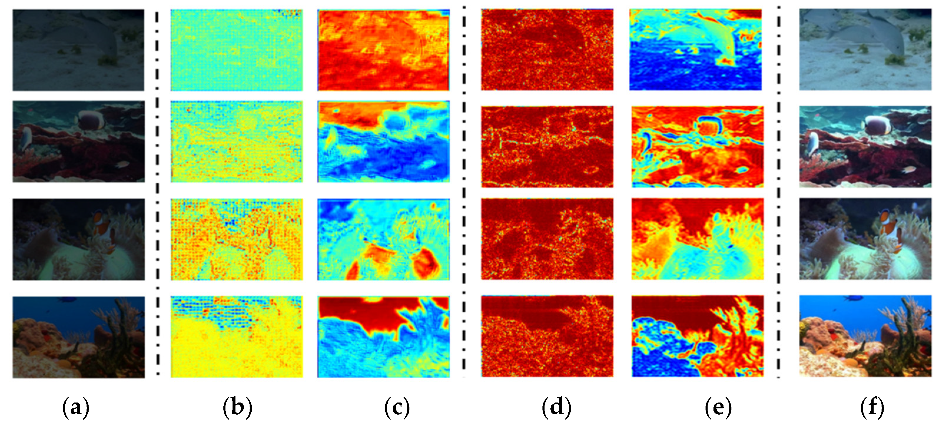
To validate the robustness of our feature extraction method, the feature visualization process was conducted in
Figure 13. These visualized features include two types of network features. Transformer features, extracted within the Token range, improve the local perception accuracy. The Transformer network captures global and long-range features through the self-attention mechanism. The self-attention mechanism allows the Transformer to integrate features from any position within the image. This is crucial for tasks such as image restoration and color correction. According to the visualized results, it is easy to find that the Transformer can effectively restore the overall color and structure of images, overcoming the defects of CNNs in the global feature-extraction process.
Conversely, CNN features provide a global perspective, contributing to improve the global perception accuracy. By visualization, it is easy find that CNNs excel at capturing the obvious features of images. Through convolution operations, CNNs can efficiently extract image details such as edges and textures, thereby effectively suppressing noise and enhancing detail. Deeper convolutional layers enables CNNs to progressively extract high-quality features from images, which is significantly effective for removing random noise in underwater images.
Furthermore, we obtained high-pass filter and low-pass filter features by the Fourier transform, which are subsequently employed as fusion weights for the two backbones’ features. High-pass filters extract edge details of image, whereas low-pass filter captures smooth information. These complementary information are multiplied with the Transformer and CNN features, respectively. This matching process enhances the accuracy of feature extraction and fusion.
Visual results show that the integration of CNNs with Transformers yields superior image enhancement effects. In summary, CNNs can remove most noise and enhance the overall color and structure, while Transformers can restore local details of the image. This combination effectively reduces noise and significantly improves the overall image quality. The effect is particularly notable when processing complicated underwater images.
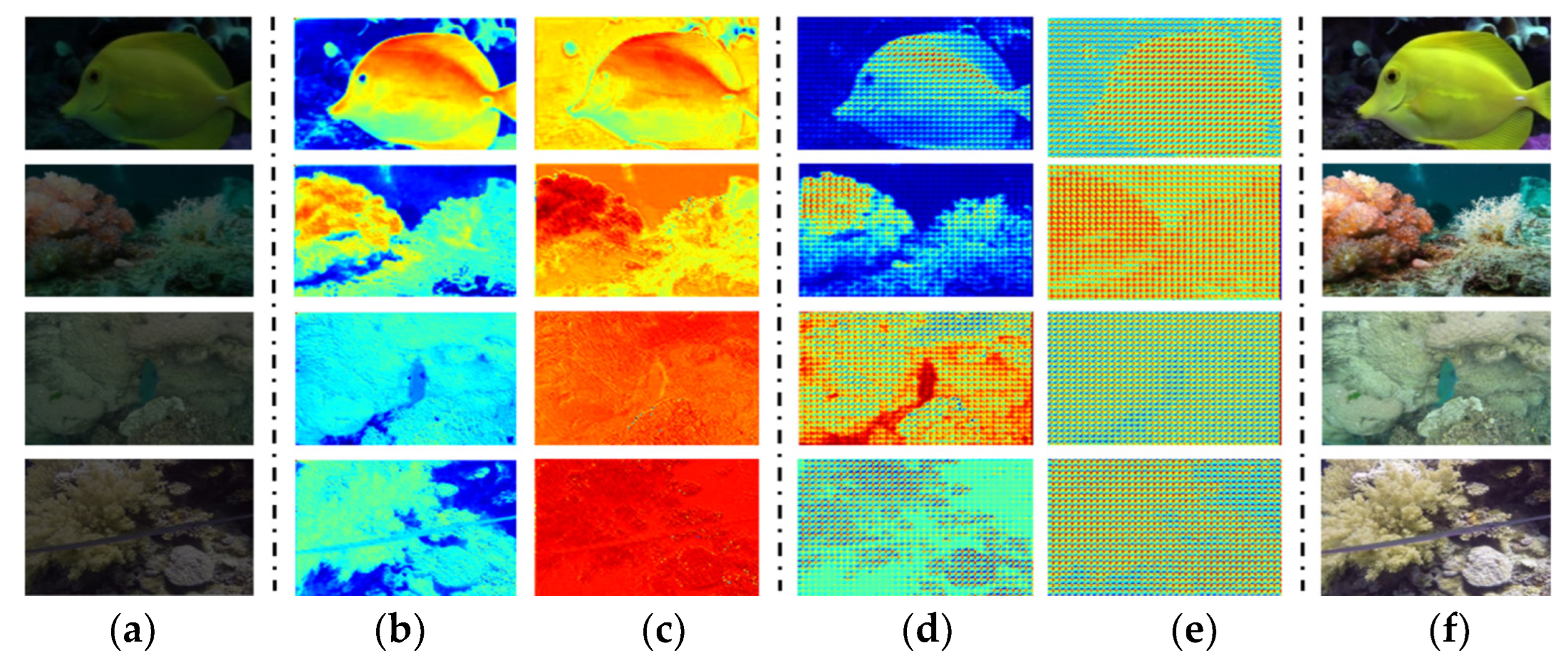
Our proposed methods are compared with other methods.
Figure 14(b) and (c) show the visualized global features, including the improved CNN network and the traditional ResNet network. The results indicate that the proposed method appears more prominent edge features, while the traditional ResNet method extracts relatively blurred features. The experiments demonstrate the superiority of proposed method that integrates both the time-domain and frequency-domain features.
Different feature
-fusion methods are also compared in
Figure 14(d) and (e). The results show that our method can optimize fusion weights for different objects, which enhances the feature diversity. In contrast, the torch.add method reduces the diversity and prominence of features.
3.4. Comparison with Current Methods
Our approach was qualitatively compared with other state-of-the-art (SOTA) image enhancement methods, including MIR-Net [
40], U-Net [
41], WaterNet [
43], and Ucolor [
44]. Additionally, the proposed backbone is compared quantitatively with the traditional CNN and Transformer architectures.
3.4.1. Qualitative Analysis
Visual samples of LSUI are displayed in
Figure 15, which are also compared with other commonly used methods. The proposed approach demonstrates the outstanding clearance, showcasing finer details, consistent colors, and higher visibility. Additionally, the method’s outputs display fewer visual artifacts, especially in zones with complicated textures.
A visual comparison of the UIEB dataset is provided in
Figure 16, highlighting our method in dealing with noisy and low-light images. The results indicate that our approach performs well in increasing image brightness, enriching image details, and suppressing noise.
3.4.2. Quantitative Analysis
In comparison to other image restoration networks, PSNR and SSIM are used to evaluate performance. Generally, higher SSIM imply the presence of more details and structure in the results. We obtained these datas from the corresponding publications or running code. All detection experiments are based on the same original input dataset, not on the optimized images from intermediate processes.
Table 4 provides a comparative analysis of various methods, indicating that our algorithm outperforms others in achieving the highest PSNR and SSIM scores.
Compared to the Transformer method [
26], it is worth noting that our linear multiplication backbone utilizes only 60% of the parameters. Additionally, in comparison with the Ucolor-based approach [
44], our method demonstrates overall superiority. Furthermore, our method outperforms MIR Net [
40], U-net [
41], and WaterNet [
43], yielding improvements of 1-3 improvement in PSNR and 0.1-0.3 in SSIM.
3.5. Comparison on Detection Tasks
To evaluate the effect of underwater image enhancement on detection tasks, the enhanced images were integrated into a series of detection algorithms, including single-stage methods SSD, RetinaNet, and GIoU [
45,
46]. These enhanced images were utilized as inputs for various detection tasks. The obtained detection results show that the proposed method exceeds other competing methods in detection accuracy. The visualized detection results in
Figure 17 correspond with the objective outcomes, demonstrating our approach’s superiority..
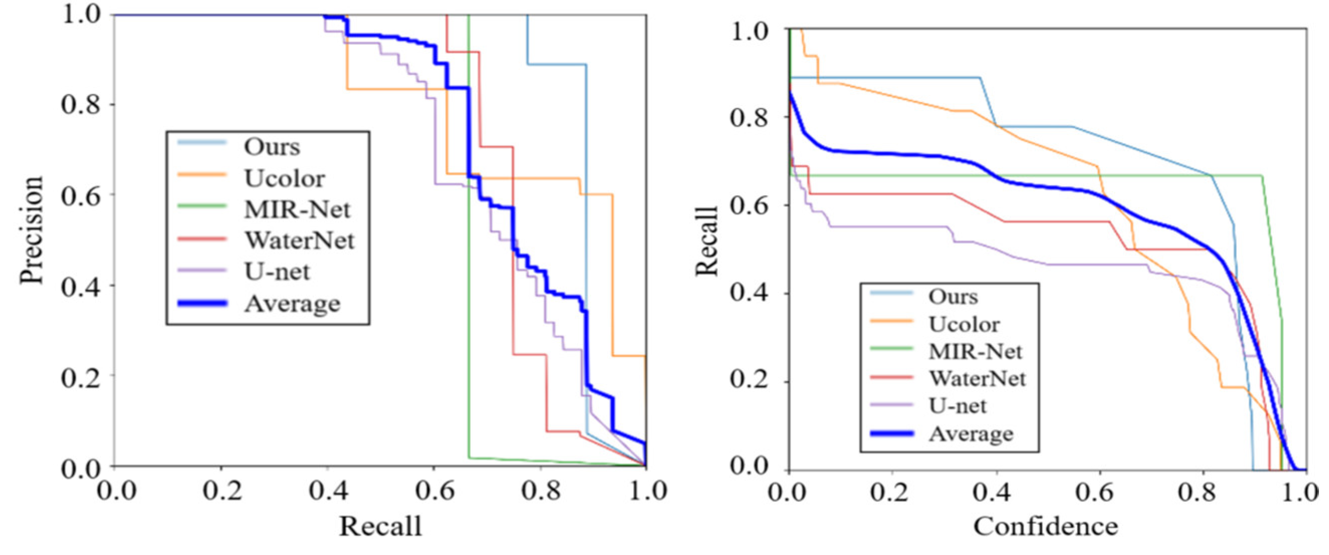
By utilizing precision-recall and recall-confidence curves as evaluation metrics,
Figure 18 presents a quantitative comparison of visual detection. Due to the improved color and brightness, our method demonstrates a notable enhancement in precision and recall indexes [
47]. The images enhanced by this method show superior detection outcomes, marking a significant enhancement over competing techniques.
Figure 1.
Visual comparisons on a real underwater image. Different methods appear different color deviation and image resolution [
3]. (a) MIR-Net. (b) U-net. (c) WaterNet. (d) Ucolor.
Figure 1.
Visual comparisons on a real underwater image. Different methods appear different color deviation and image resolution [
3]. (a) MIR-Net. (b) U-net. (c) WaterNet. (d) Ucolor.
Figure 2.
Architecture of the proposed network, which consist of three parts: encoder, fusion, and decoder.
Figure 2.
Architecture of the proposed network, which consist of three parts: encoder, fusion, and decoder.
Figure 3.
The learning process for the optimal model [
32]. (a) Convolutional Neural Network. (b) The convolutional kernels. (c) The activation functions.
Figure 3.
The learning process for the optimal model [
32]. (a) Convolutional Neural Network. (b) The convolutional kernels. (c) The activation functions.
Figure 4.
Comparisons for different CNN feature-extraction network unite. (a)The commonly used ResNet network. (b) Our feature network incorporates both temporal and frequency domain characters.
Figure 4.
Comparisons for different CNN feature-extraction network unite. (a)The commonly used ResNet network. (b) Our feature network incorporates both temporal and frequency domain characters.
Figure 5.
The transformer feature-extraction network with PSNR-based attention and linear operations. (a) The dot-product multiplication operation. (b) The element-wise multiplication operation with PSNR-based attention.
Figure 5.
The transformer feature-extraction network with PSNR-based attention and linear operations. (a) The dot-product multiplication operation. (b) The element-wise multiplication operation with PSNR-based attention.
Figure 6.
Comparison of different image block-based or modular structures. (a) The independent block’s method. (b) The proposed cross-attention method with element-wise multiplication operation.
Figure 6.
Comparison of different image block-based or modular structures. (a) The independent block’s method. (b) The proposed cross-attention method with element-wise multiplication operation.
Figure 7.
Experimental verification for different image block-based or modular structures. (a) The training loss. (b) The learned discontinuous features of independent block’s method. (b) The learned successive features of cross-attention method. (d) The PSNR and SSIM performance for different enhanced images.
Figure 8.
Fourier transformation of the image. (a) Original image. (b) Fourier transformation. (c) Shifted frequency.
Figure 8.
Fourier transformation of the image. (a) Original image. (b) Fourier transformation. (c) Shifted frequency.
Figure 9.
Low-pass filter. (a) Ideal low-pass filter. (b) Gaussian low-pass filter. (c) Low-pass filter result.
Figure 9.
Low-pass filter. (a) Ideal low-pass filter. (b) Gaussian low-pass filter. (c) Low-pass filter result.
Figure 10.
High-pass filter. (a) Ideal high-pass filter. (b) Gaussian high-pass filter. (c) High-pass filter result.
Figure 10.
High-pass filter. (a) Ideal high-pass filter. (b) Gaussian high-pass filter. (c) High-pass filter result.
Figure 11.
Comparison for different feature fusion method. (a) The commonly used torch.add method add the CNN and Transformer features. (b) The proposed approach incorporates different features with the weights of low-frequency and high-frequency features.
Figure 11.
Comparison for different feature fusion method. (a) The commonly used torch.add method add the CNN and Transformer features. (b) The proposed approach incorporates different features with the weights of low-frequency and high-frequency features.
Figure 12.
Ablation experiment with different components. (a) The same inputs for (b)/(c)/(d) detec-tion methods. (b) CNN method with Fourier transform. (c) Transformer method based on PSNR attention and linear operations. (d) CNN and Transformer fusion method with Fourier weights. (e) Ground Truth.
Figure 13.
Visualization of the features, including the transformer branch, CNN branch and fusing weights of the original image’s Fourier transform. (a) Input. (b) Transformer characters. (c) CNN characters. (d) Low pass filtering attentions. (e) High pass filtering attentions. (f) Ground truth.
Figure 13.
Visualization of the features, including the transformer branch, CNN branch and fusing weights of the original image’s Fourier transform. (a) Input. (b) Transformer characters. (c) CNN characters. (d) Low pass filtering attentions. (e) High pass filtering attentions. (f) Ground truth.
Figure 14.
Validation for the proposed methods with other commonly used structures. (a) Input image. (b) The proposed CNN network incorporates both the temporal and frequency domain characters. (c) The original ResNet only adopts the temporal characters. (d) The fused feature by the Fourier transform weight of the original image. (e) The fused feature by the torch.add method. (f)Ground truth image.
Figure 15.
Qualitative analysis with the LSUI dataset.
Figure 15.
Qualitative analysis with the LSUI dataset.
Figure 16.
Qualitative analysis with the UIEB dataset.
Figure 16.
Qualitative analysis with the UIEB dataset.
Figure 17.
Visualized detection results with different image enhancement effects.
Figure 17.
Visualized detection results with different image enhancement effects.
Figure 18.
Precision-recall and recall-confidence curves with different image enhancement effects.
Figure 18.
Precision-recall and recall-confidence curves with different image enhancement effects.
Table 1.
Computation load for different parameters.
Table 1.
Computation load for different parameters.
| Parameters |
Computation load |
Computation load summation |
|
d*n |
3d*n |
| q |
d*n |
|
d*n |
Table 2.
Comparative test of ablation experiments.
Table 2.
Comparative test of ablation experiments.
| Structures |
Fusion |
LSUI |
UIEB |
| CNN |
Fourier |
Transformer |
SNR attention |
Additive fusion |
Fourier fusion |
PSNR |
SSIM |
PSNR |
SSIM |
| ✓ |
|
|
|
|
|
15.22 |
0.47 |
13.03 |
0.42 |
| ✓ |
✓ |
|
|
|
|
18.82 |
0.64 |
16.77 |
0.60 |
| ✓ |
✓ |
✓ |
|
|
✓ |
24.83 |
0.79 |
21.70 |
0.70 |
| ✓ |
✓ |
✓ |
✓ |
✓ |
|
24.42 |
0.75 |
21.56 |
0.69 |
| ✓ |
✓ |
✓ |
✓ |
|
✓ |
26.53 |
0.83 |
23.85 |
0.78 |
Table 3.
Comparison of different matrix-multiplication attention and computation latency.
Table 3.
Comparison of different matrix-multiplication attention and computation latency.
| Backbones |
Attention |
Latency(ms) |
| Transformer |
Dot-product Transformer |
2.5ms |
| Element-wise Transformer |
2.1ms |
| Transformer + CNN |
Dot-product Transformer |
3.0ms |
| Element-wise Transformer |
2.6ms |
Table 4.
Comparative evaluation with different image enhancement networks.
Table 4.
Comparative evaluation with different image enhancement networks.
| Methods |
LSUI |
UIEB |
| PSNR |
SSIM |
PSNR |
SSIM |
| CNN[16] |
15.28 |
0.50 |
13.68 |
0.48 |
| MIR-Net[40] |
18.80 |
0.66 |
16.78 |
0.63 |
| U-net[41] |
19.45 |
0.78 |
17.46 |
0.76 |
| WaterNet[43] |
19.62 |
0.80 |
19.27 |
0.83 |
| Ucolor[44] |
21.62 |
0.84 |
20.67 |
0.81 |
| Transformer[26] |
22.83 |
0.79 |
21.70 |
0.70 |
| Ours |
24.49 |
0.85 |
22.79 |
0.81 |

