1. Introduction
In this research, we propose an integration of machine learning (ML) techniques with a physics-based Lagrangian model [
1] to address environmental issues of sea surface debris. At the core of this study is a pipeline that uses historical data to predict the next 24 hours of sea surface currents (SSC) velocities. These predictions serve as inputs to a Lagrangian model, enabling it to simulate the movement of surface marine debris. Finally, a comparative evaluation of both LSTM and GRU models is conducted, focusing on their predictive accuracy and the quality of the visualisations. This offers valuable insights to marine conservation efforts and enhances decision-making processes for the management of marine debris around the Maltese Islands.
1.1. Problem Definition
Sea surface debris around the coastal waters of Malta presents a significant environmental issue. Predominantly composed of plastics, which constitute 82% of all man-made floating materials encountered in the Mediterranean Sea [
2], this debris endangers marine life, disrupts ecological balances, and compromises the ecological integrity of coastal areas [
3]. Studies reveal significant negative effects, ranging from harm to marine wildlife due to ingestion and entanglement [
4], to the disruption of natural habitats [
5]. The impact on coastal ecosystems extends beyond the environment, affecting economic sectors reliant on marine health, such as tourism and fishing [
5]. Further research covers the long-term ecological consequences, highlighting the urgent need for effective management and mitigation strategies as discussed in [
6]. This problem is further aggravated by the lack of an effective system that can predict the movement of this surface debris since, as of this writing, there exists no system that addresses this challenge for the coastal areas around Malta. This underscores the need for a system that can accurately predict and visualise the dispersion patterns of sea surface debris.
1.2. Motivation
The geological characteristics of the Mediterranean Sea make it difficult for surface debris to escape the area naturally, resulting in it accumulating [
7]. The current absence of a predictive system tailored to the coastal regions of Malta impedes effective interventions to mitigate environmental harm. This gap opens an opportunity for the implementation of a system that aims to address an urgent ecological issue, which is widely recognised as a global crisis [
8]. By fulfilling this need, this research aims to provide accurate predictions that can guide effective cleanup operations and inform strategies for long-term marine conservation around the coast of Malta.
1.3. Aims and Objectives
This study aims to create a system that simulates and predicts the movement of marine debris in the coastal waters of Malta, thereby supporting marine conservation efforts. To achieve this, several objectives have been identified. The sea surface currents (SSC) velocity datasets obtained from the HF Radar Network operated and maintained by the Department of Geosciences at the University of Malta will be preprocessed and organised to ensure compatibility and consistency for input into the ML and Lagrangian models. The ML models are necessary to predict future SSC velocities, and the Lagrangian physics model will be used to accurately simulate debris movement and dispersal. Following extensive experimentation, we find that LSTM and GRU models hold the most promise in terms of accuracy and real-time performance. As such, we will evaluate both models to determine which one is able to predict sea surface currents better. Beyond assessing the accuracy of our models, we also perform a more detailed geospatial analysis to better understand the conditions which make one model perform better than the other. The source code and datasets used in this study are publicly accessible on GitHub
1.
2. Materials and Methods
2.1. The SSC Dataset
In this study, we utilise a dataset provided by the Department of Geosciences at the University of Malta
2. This dataset consists of SSC velocities data, recorded in hourly increments across four years, spanning from January 2020 to December 2023. These data points are derived from high-frequency (HF) radar systems [
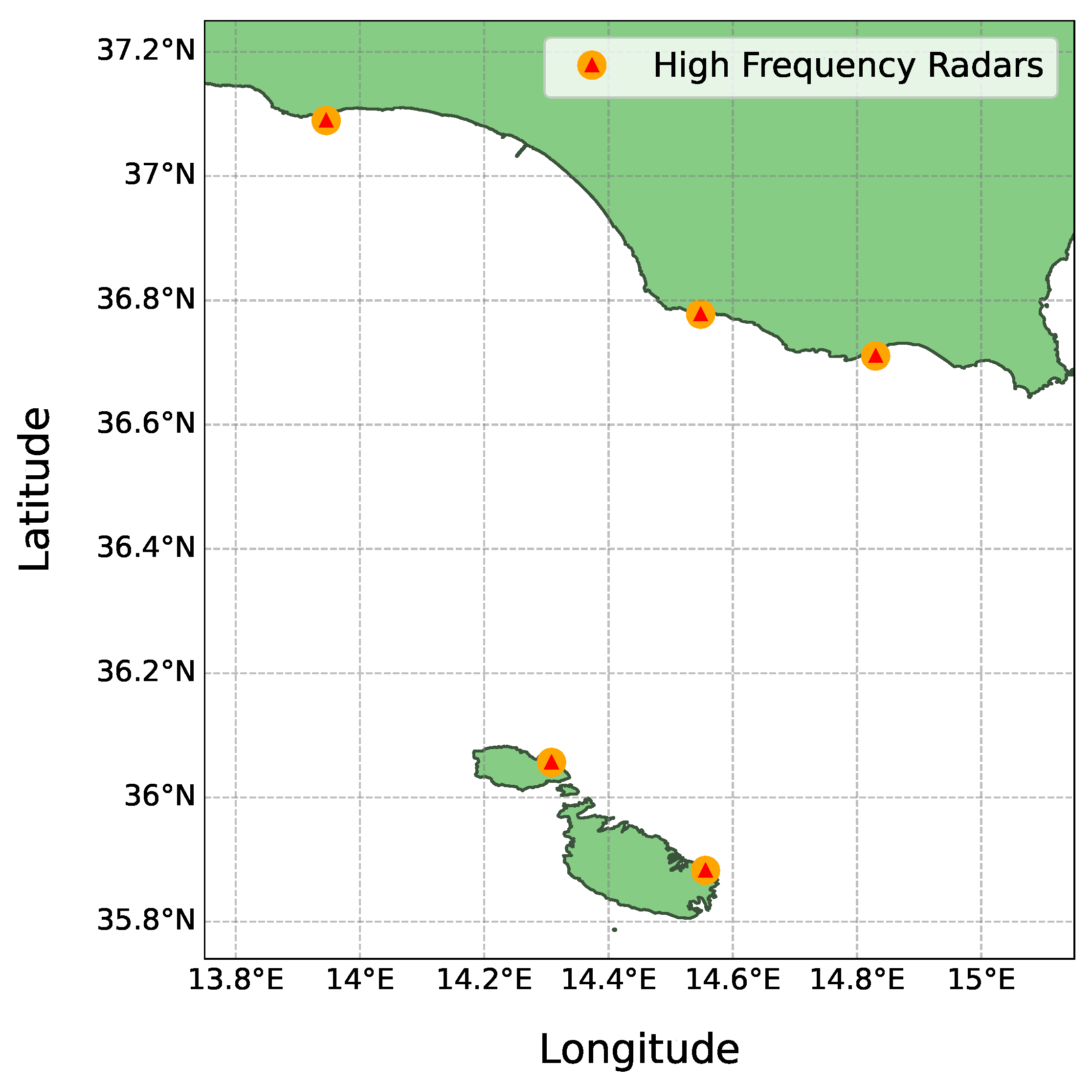
9], located in the northern regions of the Maltese Islands and southern Sicily. The locations of these radar systems, depicted in
Figure 1, provide a temporal snapshot of the SSC movements.
The data is composed of several variables including longitude, latitude, time, and SSC velocities denoted by the west-east velocity (
u) and the north-south velocity (
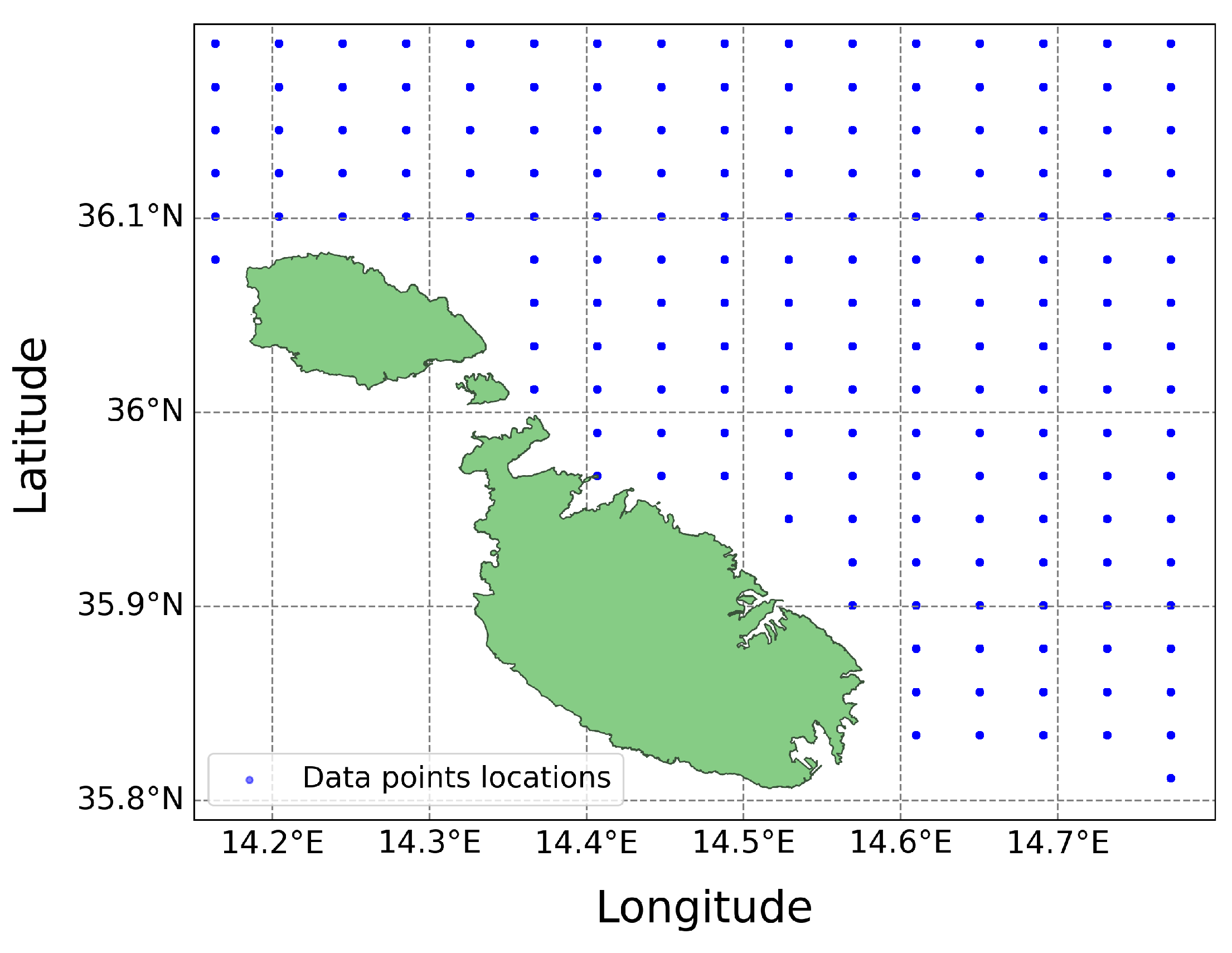
v). The data’s geographical scope is defined within the boundaries of 14.15°E to 14.81°E longitude and 35.79°N to 36.30°N latitude. This coverage translates into a grid totalling 180 data points, as shown in
Figure 2. The dataset is in Network Common Data Form (NetCDF) format [
10], a commonly used format for climate and meteorological data, ensuring compatibility with the Lagrangian Model.
2.2. The Lagrangian Model
The practice of tracking ocean surface movements in a Lagrangian framework dates back to the earliest days of oceanography. Early methods involved observing the drift of ships or the paths of specially designed floats to document sea current movement, as outlined by [
11]. The Lagrangian model [
1] plays a pivotal role in environmental simulations. By offering a dynamic method to trace individual particle trajectories within fluid mediums, the model ensures precise tracking of the particle’s spatiotemporal movement. Its broad applicability spans from localised studies to global-scale systems. This is evident in its varied applications, such as tracking oil spill diffusion [
12], mapping floating plastic debris [
13], simulating jellyfish migrations [
14], and smoke dispersion [
15].
The Lagrangian model operates by representing particles within a fluid medium, tracking their position and properties as they move with the fluid’s flow. The model calculates each particle’s trajectory by integrating the fluid’s velocity field, which may vary in time and space. This approach enables the simulation of dispersal patterns of particles, such as marine debris, by accounting for both advection and diffusion processes. Advection represents the movement of particles by the flow of a fluid [
16]. Diffusion, on the other hand, models the dispersion of particles through random motion [
16]. This is done by applying techniques such as random walks or Gaussian distributions. This inclusion of randomness enhances the realism of the simulations.
To facilitate these Lagrangian simulations, several Python toolkits like OceanParcels [
17], PyGnome [
18], and Flexpart [
19] have been developed. These toolkits enable the customisation and execution of particle tracking simulations, leveraging data on ocean currents, wind fields, and other environmental phenomena. OceanParcels is distinguished by several features that make it suitable for our work. One of its notable capabilities is custom kernels. These are user-defined functions that allow for tailored simulation scenarios at each time step. Through custom kernels, users can implement complex behaviours and interactions of particles within the fluid, such as particle reflection or response to environmental variables like temperature and wind. Another significant feature is particle initialisation. This feature enables the creation of particles at specific locations, times, and with distinct properties, allowing for more detailed and accurate simulations.
2.3. Time Series Modelling
Time series modelling is a technique used to predict future data points by analysing the trends, cycles, and patterns in a series of data points collected over an interval of time [
20]. The main focus is on analysing historical data to uncover the underlying structure of the data, which can then be used to forecast future trends. This method is particularly powerful for its ability to incorporate the sequence and time dependence within a dataset. By examining how values are interconnected over time, time series models can forecast future values based on the inherent temporal dynamics present in the historical data [
21]. This form of predictive modelling assumes that past patterns shape future behaviours, making it an indispensable tool in various fields ranging from weather forecasting [
22] to stock market predictions [
23].
While time series modelling is a powerful tool for forecasting future data, it also has its challenges and limitations. Time series data often exhibit seasonality and trends, which can complicate the forecasting process [
24]. Outliers, missing sequences of data, and anomalies can also significantly impact the accuracy of forecasting models, requiring careful identification and handling. The capacity of these models to integrate external influential factors and variables is also somewhat limited, often necessitating the integration of additional features for enhanced predictive accuracy [
25]. Additionally, time series models require significantly more data for training, which can be cumbersome in situations where data is limited [
25]. These challenges highlight the importance of adopting a methodical approach to time series modelling, emphasising the need to carefully consider the specific context and characteristics of the data being analysed when utilising time series models for effective forecasting.
In the context of our work, we use time series modelling to predict SSC velocities. Accurate predictions require a detailed analysis of the data sequences to discern patterns that could forecast future predictions. The historical hourly data of SSC form a time series, which is inherently continuous but sampled at discrete intervals. To address this, we use long short-term memory (LSTM) and gated recurrent unit (GRU) models due to their competence in handling vast amounts of sequential data and their capacity to learn complex temporal patterns [
26,
27,
28]. After training on past SSC data, these models can predict future values with good accuracy.
2.4. Data Integration and Preprocessing
The raw data is split into multiple folders and sub-folders for each day, necessitating a robust method to merge and preprocess the data without interfering with its temporal and spatial dimensionality.
To address this, we developed a utility that allows us to specify the start and end dates for the merging of the SSC data. This then merges the individual files along the time dimension, creating a single dataset that encompasses all relevant data across the specified interval. This merged dataset is not only more manageable but also streamlined for any subsequent processes. A key feature is the preservation of the geographical boundaries and temporal aspects of the data. The dataset maintains the latitude and longitude ranges, ensuring that the spatial integrity is uncompromised. Furthermore, checks are performed to ensure the time remained consistent, preserving the temporal integrity of the data.
Upon analysing the data, a substantial number of missing values, represented as not-a-number (NaN), were discovered. These NaNs are likely due to the proximity of the data to the coast, where high-frequency radars often struggle to capture all the data accurately. We decided not to address these NaN values at this stage. Each objective requires tailored handling of missing data, which will be discussed in the next sections.
2.5. The Lagrangian Model Development
Due to the strengths highlighted in 2.2, the OceanParcels toolkit [
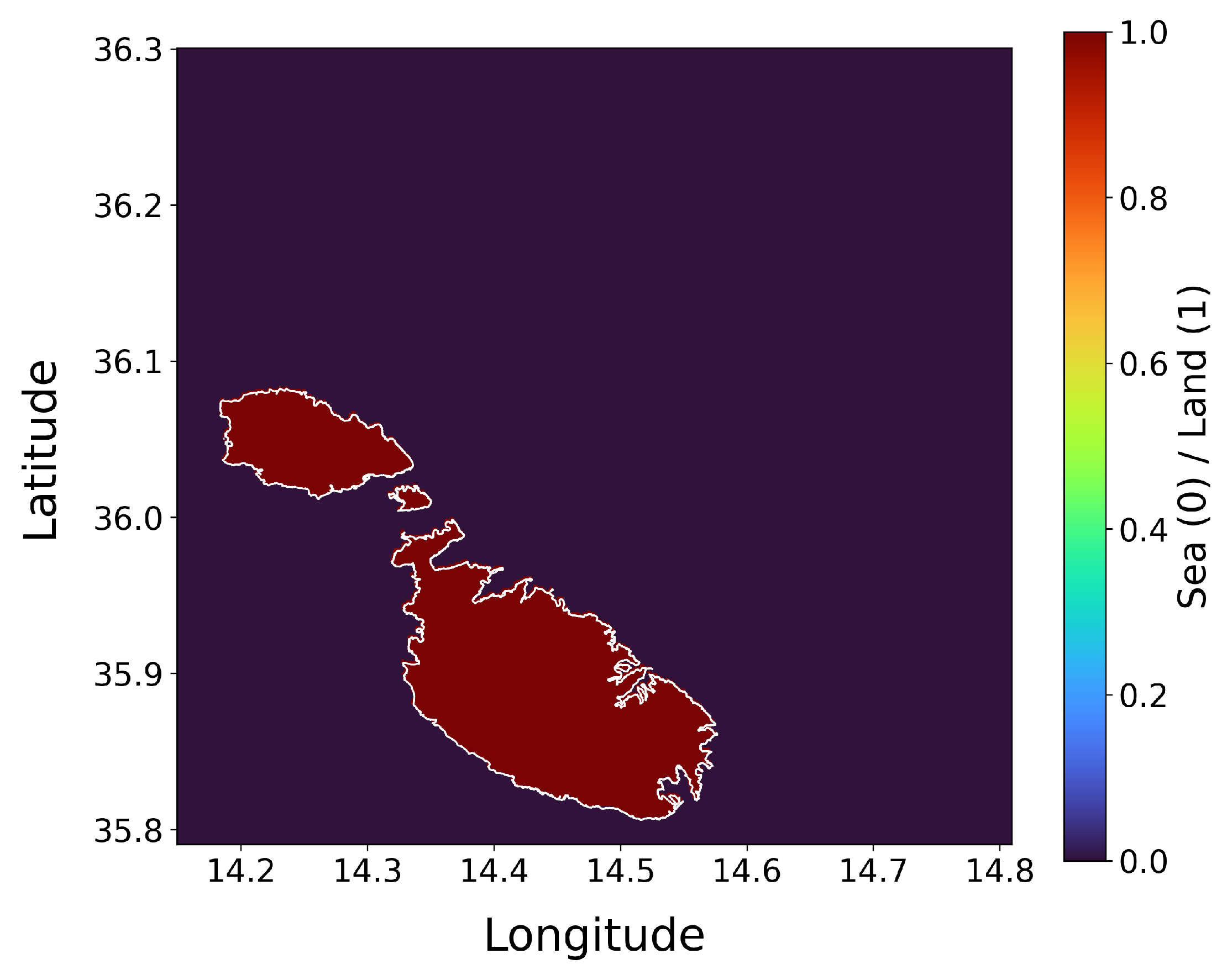
17] was chosen for this study. The first step was to create the land-sea mask as can be seen in
Figure 3. This effectively differentiates land from sea, ensuring accurate particle behaviour. The mask was saved as a NetCDF [
10] file and added within the grid boundaries to match with the boundaries of the dataset. These coastal boundaries define the simulation area and facilitate land-sea interactions.
Subsequently, a
FieldSet was created from the SSC dataset. This serves as the simulation environment, defining the velocity fields that drive particle movement. Additionally, the land-sea mask was integrated into the
FieldSet, providing necessary data for handling particles upon reaching land. As depicted in
Figure 4, simulation particles were initialised near a specific geographic coordinate (36.0475°N, 14.5417°E), with random offsets to simulate a dispersed release. The particles represent the objects of interest, such as sea surface debris, whose movements will be simulated. Initially, the strategy involved simulating numerous randomly placed particles across the entire area; however, to enhance realism, we placed a cluster of 50 particles in close proximity. This configuration was selected to accurately represent how debris navigates marine environments, with each particle representing a cluster of debris.
Custom kernels are a critical component of the simulation and allow us to introduce specific behaviours into the simulation, thereby modelling realistic scenarios that particles may encounter. The behaviours implemented include:
CheckOutOfBounds: deletes particles from the simulation if they move beyond the defined boundaries. This is necessary because no data is available outside the boundary, causing particles to get stuck.
CheckError: deletes particles encountering computational errors. This ensures the simulation proceeds without disrupted or incorrect particle data.
UpdateElapsedTime: shows how long a particle has been in the simulation. This tracks the duration of the particle within the environment.
UpdatePreviousPosition: captures the position of particles before they move. This is useful as it allows us to save all the previous positions of the particles.
ReflectOnLand: applies a reflection behaviour when particles encounter land, as defined by the land-sea mask. It also introduces a probabilistic component where there is a 15% chance that particles will `beach’ and be removed from the simulation, while the remaining 85% chance allows particles to be reflected back into the sea. This probabilistic distribution is justified by the geographic characteristics of Malta, where the predominance of rocky coastlines over sandy beaches increases the likelihood of debris being deflected back into the sea rather than getting beached.
The simulation was executed, and the resulting particle movements and dispersion patterns were visualised. These visualisations provide valuable insights into the trajectories of particles and their interactions with the environment. The time-step for the Lagrangian simulation was set to 10 minutes, capturing the continuous dynamics of particle dispersion. This interval provides a good balance between computational efficiency and accuracy. The results were saved as an animated GIF file, offering a dynamic and easily interpretable visual representation of the simulated particle dispersion over time.
Some challenges emerged during this part of the implementation. Initially, simulations revealed that particles were getting stuck at the border boundaries. This issue was traced back to the dataset, which lacked data at the borders, rendering the particles unresponsive to environmental variables in these areas. To address this, the boundary of the simulation area was slightly reduced by 0.1° in longitude and latitude. The simulation was defined over a seven-day period (longer periods were unreasonable and did not align with the research goals). To achieve this, the preprocessing steps discussed in
Section 2.4, were utilised to merge the data from 1
st January to 7
th January 2023. Wind was not considered in the simulation as the spatial distribution of microplastics does not appear to be significantly affected by it. This intuition is supported by the research done by M. Erikson et al. [
29]. Despite this, it may still be possible that wind data may enhance the accuracy of the simulations in depicting real-life scenarios and may be an interesting improvement.
To deal with the missing data an attempt was made to interpolate the missing values. The visualisation results were noticeably different from those produced using the raw data which included NaNs. Despite experimenting with both linear and spline interpolation, the outcomes of the interpolated simulations remained consistent across different time frames, suggesting that the interpolation was excessively homogenising the data. This uniformity introduced by interpolation was misleading, as it failed to represent the true variability and dynamics of the SSC, compromising the actual behaviour and movement patterns of particles in the sea. Consequently, it was decided not to remove NaN values from the data used in the Lagrangian simulations. This decision was based on the understanding that removing or interpolating these values could lead to simulations that do not accurately reflect real-world conditions. By preserving the integrity of the original dataset, including its inherent gaps, the simulations were more likely to represent the actual conditions and variations that marine debris would encounter in the sea. Examples of the final visualisations are presented in
Figure 11 and
Figure 19.
2.6. ML Model Selection
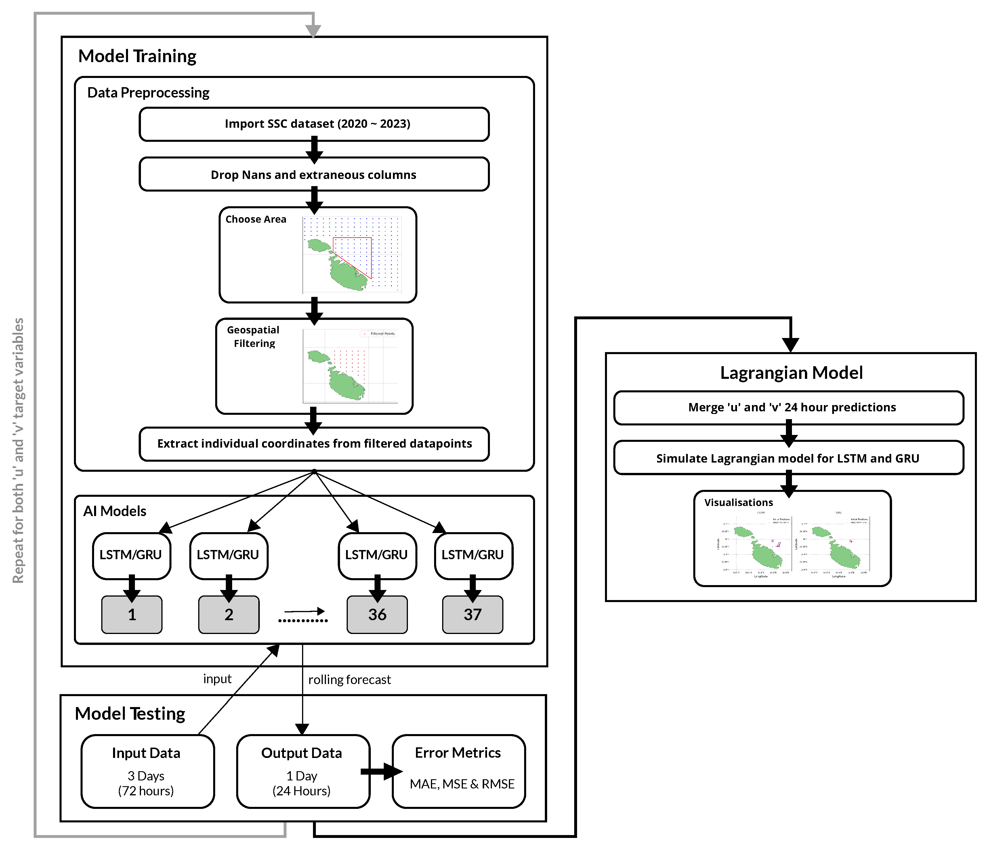
A pipeline (
Figure 10) was established to predict the SSC velocities. The initial phase involved selecting appropriate models, with LSTM and GRU architectures identified as the optimal choices. This decision was informed by their demonstrated effectiveness in processing time-series data, rendering them particularly suitable for this task, as shown in studies by A. M. Ali et al. [
30] and I. I. Zulfa et al. [
31]. By utilising these models, we can accurately predict the dispersion of marine debris around Malta’s coastal waters, addressing both the temporal dynamics and spatial complexities inherent in SSC movements.
2.6.1. Data Preprocessing and Geospatial Filtering
While the initial plan was to train a model on a year’s worth of data to forecast SSC for the next month, the complexity and four-dimensional nature of the data led to sub-optimal predictions. Consequently, the strategy was revised to extend the dataset used for training, which spanned from February 25
th 2020 to August 1
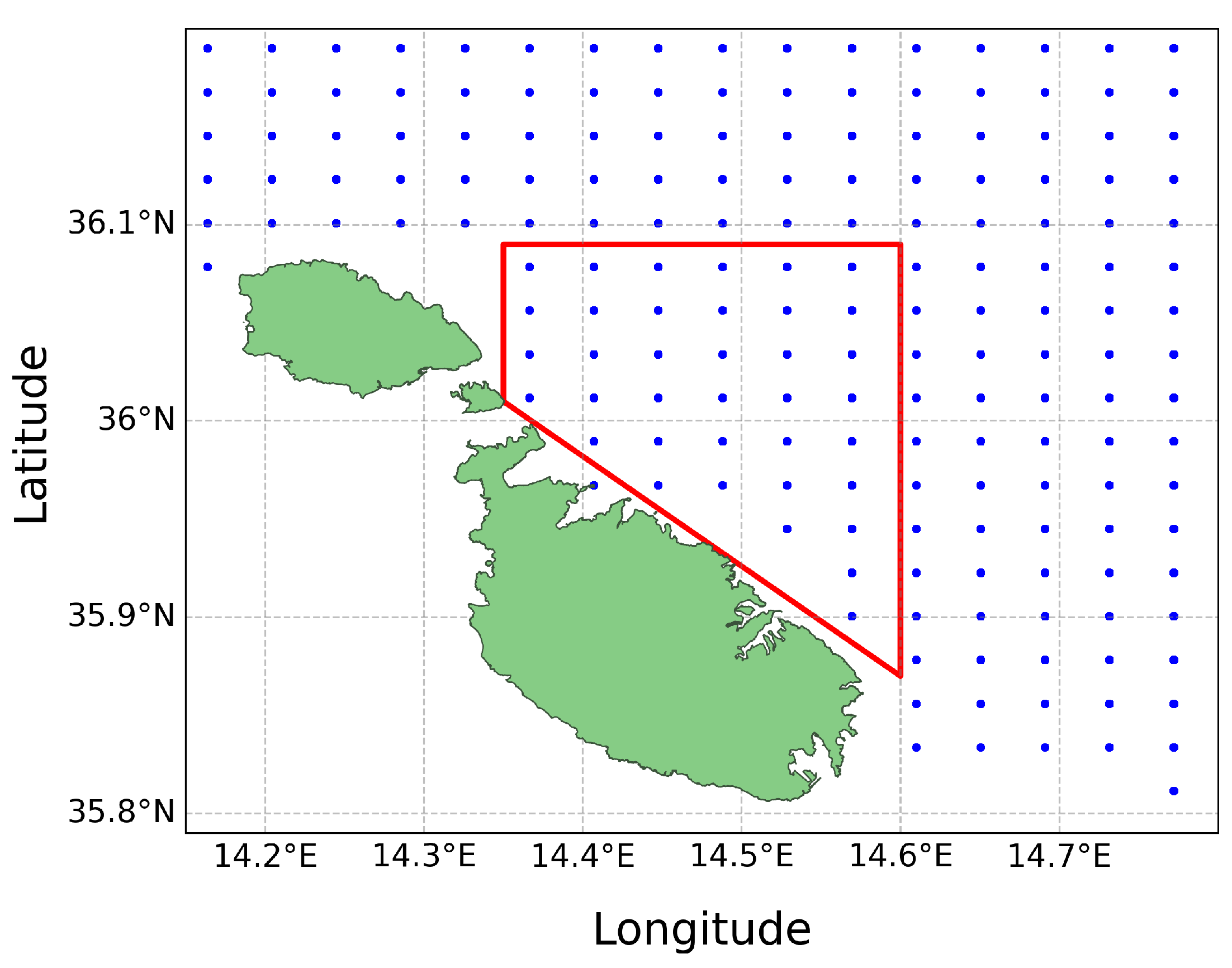
st 2023. Given the substantial volume of data points and the need for geospatial filtering, a decision was made to concentrate on a smaller area of interest along the northern coast of Malta, as illustrated in
Figure 5. The method involved predicting the
u and
v components individually for each longitude and latitude pair within the defined area. These individual predictions were subsequently merged into a single file and finally inputted into the Lagrangian simulation.
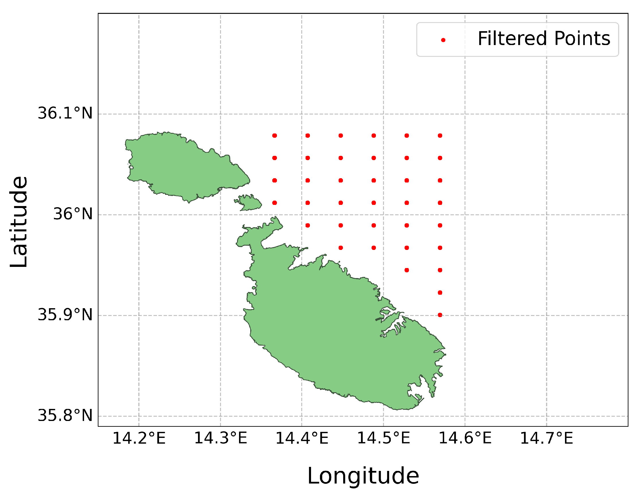
The dataset was geospatially filtered to only include data points within the designated area of interest, as shown in
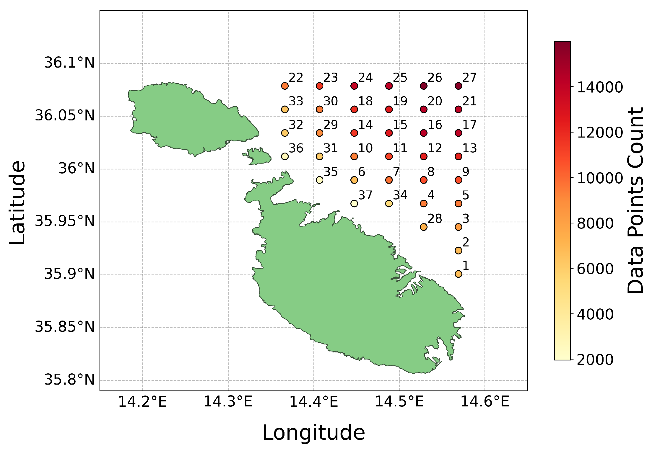
Figure 6. This filtering resulted in a focused dataset consisting of 37 data points. The data did not require any normalisation as it had already been scaled between -1 and 1 during the data collection phase. Each coordinate pair was then processed into individual comma-separated-values (CSV) files. These files were systematically named and organised according to the corresponding latitude and longitude coordinate points. These CSV files served as the basis for training the AI models for every individual data point location.
Areas closer to the coast had fewer data points (more NaNs), as illustrated in the heat map in
Figure 7. This lack of data near coastal regions is likely attributed to several factors. These include radar interference from nearby land or structures, obstruction of radar beams by coastal terrain or buildings, and refraction of radar waves at the coast, all contributing to distorted data collection. Efforts to solve this issue included experiments with data interpolation and filling missing values with the mean. However, these methods yielded worse results compared to those obtained by eliminating the NaN values. Due to this, the most effective strategy proved to be the removal of NaN values, a decision informed by testing and alignment with the methodologies applied for the Lagrangian model, as discussed in
Section 2.5.
Prior to creating the pipeline, preliminary testing was conducted on a single model to determine the most effective features and targets. Experimentation involved the integration of both u and v as features, revealing marginally improved outcomes compared to using each as a single feature, prompting a focus on using both features for the predictions. Notably, the model yielded good results when predicting a single target, but the accuracy of predictions noticeably diminished upon testing the model to predict both u and v as targets. This observation led to the decision to develop separate models for each target variable to maximise the accuracy of the results. Therefore, we implemented a series of 37 models to predict the u component and repeated this process for the v component, ensuring precise and reliable predictions.
2.6.2. The Main Loop
Inspired by the approach of H.-M. Choi et al. [
32], who developed a model for every individual coordinate pair, we established a pipeline that iterates through each pair of coordinates in the dataset (total of 37) and trains a dedicated model for each individual pair. This approach made possible the predictions across the entire area of interest, which are later utilised for the Lagrangian simulations. The
u and
v columns in the data files prepared earlier are extracted as input features. The dataset is then divided into training, validation, and testing sets in a 70-15-15 split respectively, a common split for ensuring a balance between adequate model training and thorough evaluation. Given the time series nature of the data, it was necessary to sequence the data appropriately; this was achieved using the
TimeseriesGenerator library
3. Iterative testing of different parameter combinations revealed that a window size of 72 hours, a batch size of 64, and a sampling rate of 1 unit yielded the best overall results. This means that the data is sequenced into continuous blocks of 72 hours of data as input and paired with the value immediately following these 72 hours as the target output. This step allows the model to predict the next hour based on the preceding 72 hours of data.
TensorFlow
4 was used to implement the models. Various architectures and hyperparameters were tested to determine which ones yielded the best results, including a partial grid search for hyperparameter tuning. To ensure a fair comparison, we applied identical hyperparameters and layer configurations across both the LSTM and GRU architectures. The most effective architecture involved ten hidden layers, composed of four LSTM/GRU layers, three dropout layers, and two dense layers activated by
ReLU, followed by an additional dropout layer after each dense layer. The models were set up with a learning rate of 0.001,
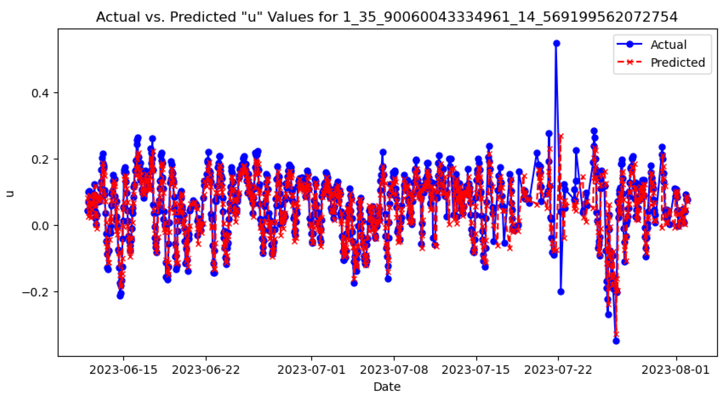
ADAM optimiser, and the MSE loss function. Importantly, the model was reinitialised in each iteration of the loop, ensuring that each dataset was trained on a fresh instance without any residual weights from previous iterations. This approach is crucial when dealing with multiple datasets to avoid any data leakage or influence from previously trained models (clean slate training). It also helps maintain the integrity of the learning process for each distinct dataset. Early stopping with a patience of 8 epochs was implemented to halt training and prevent overfitting. Model checkpoints were utilised to save the best-performing epoch automatically. After each training epoch, plots comparing training versus validation loss were generated to monitor the performance of each model. To ensure that each model was trained adequately, predictions were made on the test set and subsequently visualised by comparing actual versus predicted values, as illustrated in
Figure 8. Finally, adopting a similar evaluation approach to Adhikari et al. [
20], MAE, MSE and RMSE error metrics were computed and displayed to evaluate the model’s performance on the test set.
2.6.3. Making Real-World Predictions
In the final phase of the AI model pipeline, we undertook a simulation mirroring a real-world scenario by feeding historical data spanning 72 hours to predict the subsequent 24 hours. This 24-hour prediction window is chosen as it provides a balance between short-term accuracy and computational feasibility, which is typically used for time series forecasting in dynamic environments like SSC. The dates of 4
th August and 4
th November 2023 were selected to assess the model’s performance under different seasonal conditions, from here on referred to as
Test 1 and
Test 2 respectively. Specifically, data from 1
st to 3
rd August 2023 were used as input to predict conditions for
Test 1, data from 1
st to 3
rd November were used for
Test 2. This setup allowed us to compare the predictions with actual historical data from our dataset. The process began with a loop to systematically extract SSC data across 72 hours for all 37 individual coordinate pairs. Subsequently, actual observed data for the following 24-hour period on 4
th August (
Test 1) was extracted for comparative purposes, and both sets were saved as CSV files. Given the requirement for 72 consecutive hours of data to be able to make predictions and 24 hours for comparison, spline interpolation
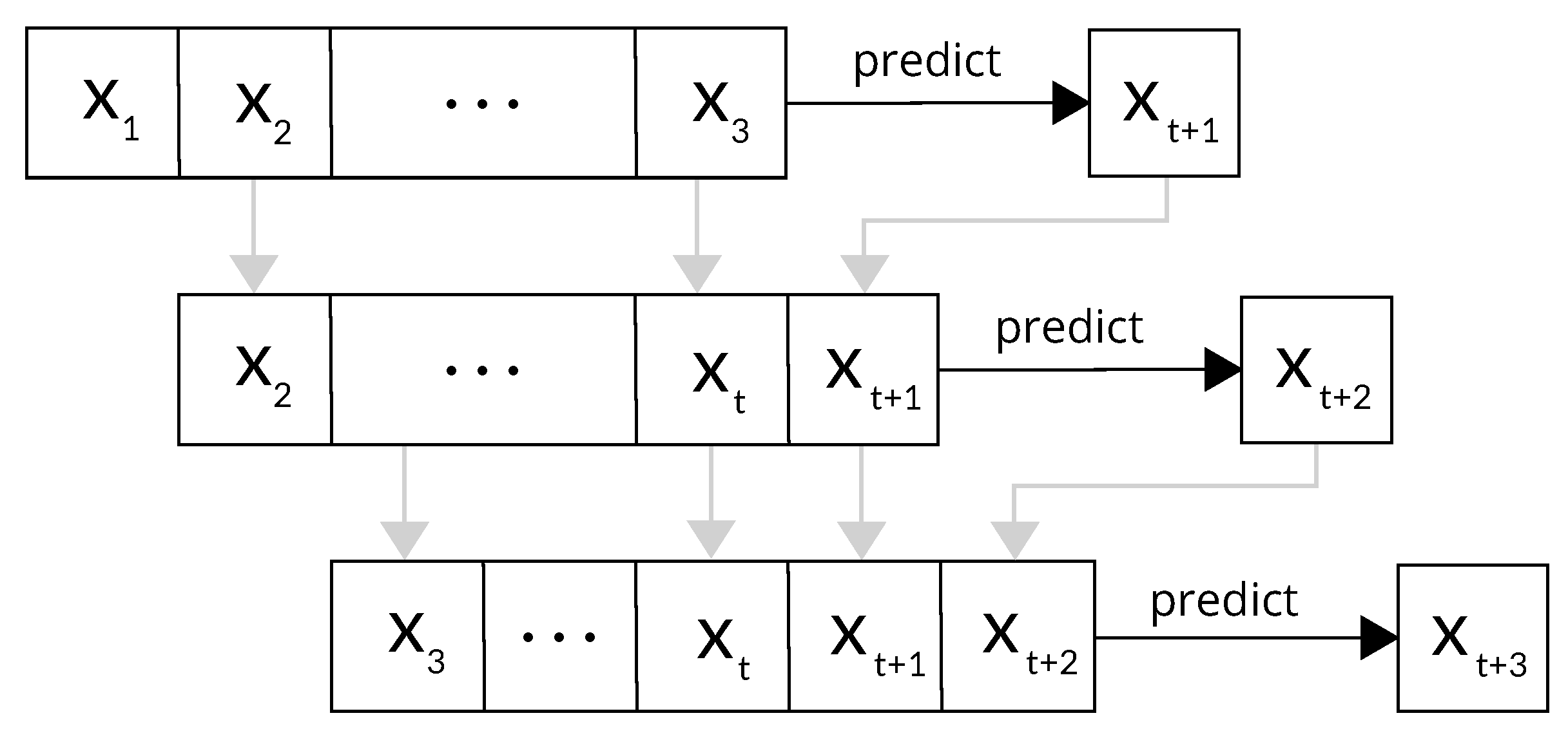
5 was utilised to address any present NaN values, ensuring the dataset’s completeness. Using the rolling forecasting method shown in
Figure 9, predictions were generated for the subsequent 24-hour period for the individual targets
u and
v. We note that predictions based on interpolated data serve as inputs for subsequent forecasts, potentially diminishing their precision. This effect is particularly noticeable in longer-term predictions, where accuracy tends to decrease as the forecast horizon extends, expectedly showing a decline in prediction accuracy the further the prediction extends into the future.
This process was repeated for all 37 data points and the predictions are converted into NetCDF format to be subsequently used in the Lagrangian model. Finally, the same error metrics were calculated to be used later for evaluation. This pipeline is repeated four times, encompassing two LSTM models and two GRU models, one for each of the
u and
v components respectively. The architecture of the AI models pipeline is illustrated in
Figure 10 below:
Figure 10.
Overview of the entire pipeline.
Figure 10.
Overview of the entire pipeline.
2.7. Integrating the ML Models with the Lagrangian Model
The final stage of the pipeline involves integrating the AI models’ predictions with the physics-based Lagrangian model to produce a 24-hour forecast simulation of sea surface debris dispersion.
This process was conducted separately for both the LSTM and GRU model predictions. The initial and most critical step involves the preprocessing and merging of the predicted
u and
v values as NetCDF data. Following this, the procedures outlined in
Section 2.5 were implemented once again to set up the Lagrangian simulation framework. This involved the configuration of the land-sea mask,
FieldSet, number of particles, kernels, and timestep. The only difference lies in the particle initialisation phase. Given that the AI model predictions were specific to the area of interest (as depicted in
Figure 6), we decided to set the centroid of the polygon as the starting position. More specifically, the coordinates are at a latitude of 35.9895° and a longitude of 14.4944°. This approach is advantageous as it allows for an unbiased observation of dispersion patterns. The reason being, that since the centroid is equidistant from all edges of the polygon, it provides a neutral starting point that does not inherently favour any flow direction. In terms of the offset of the initial particles, the same random seed was used for both LSTM and GRU simulations. This ensures a fair comparison as the initial locations of the particles are identical for both models.
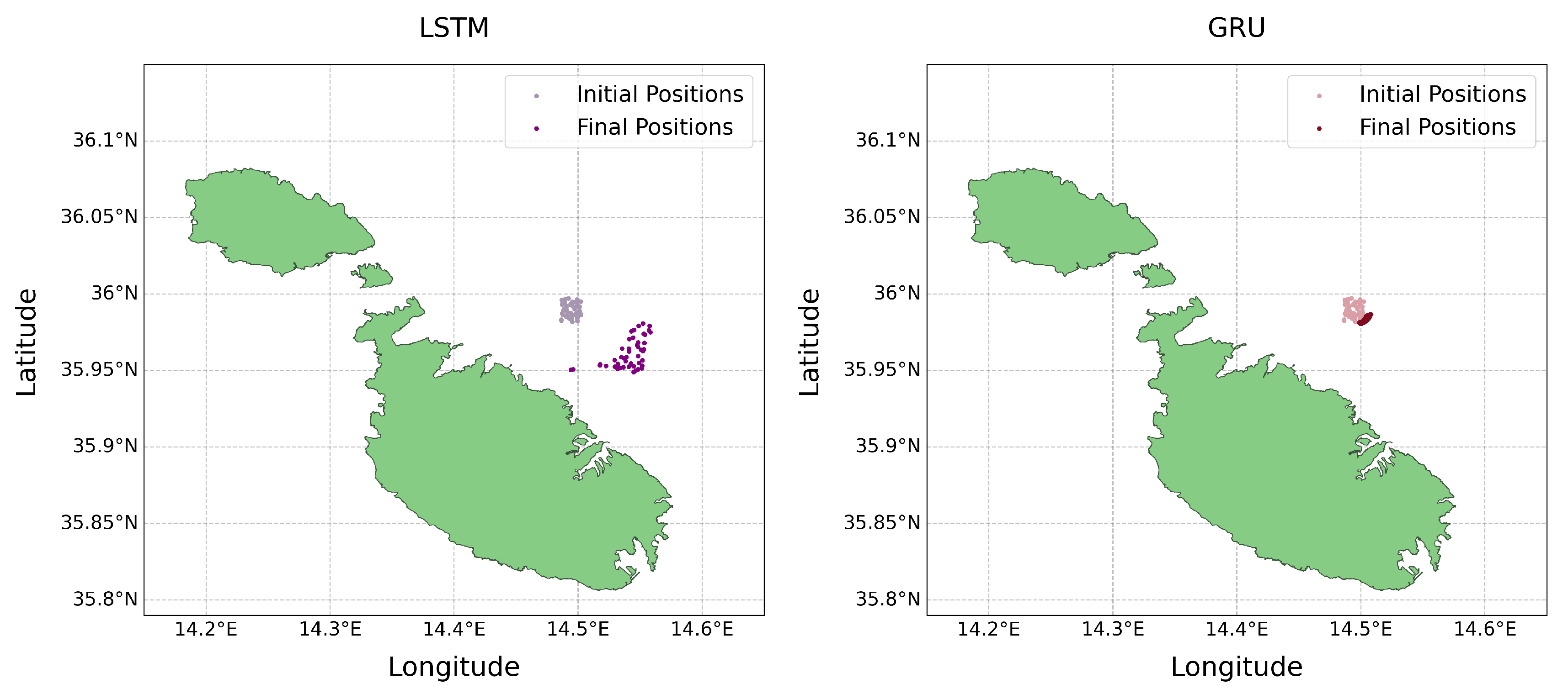
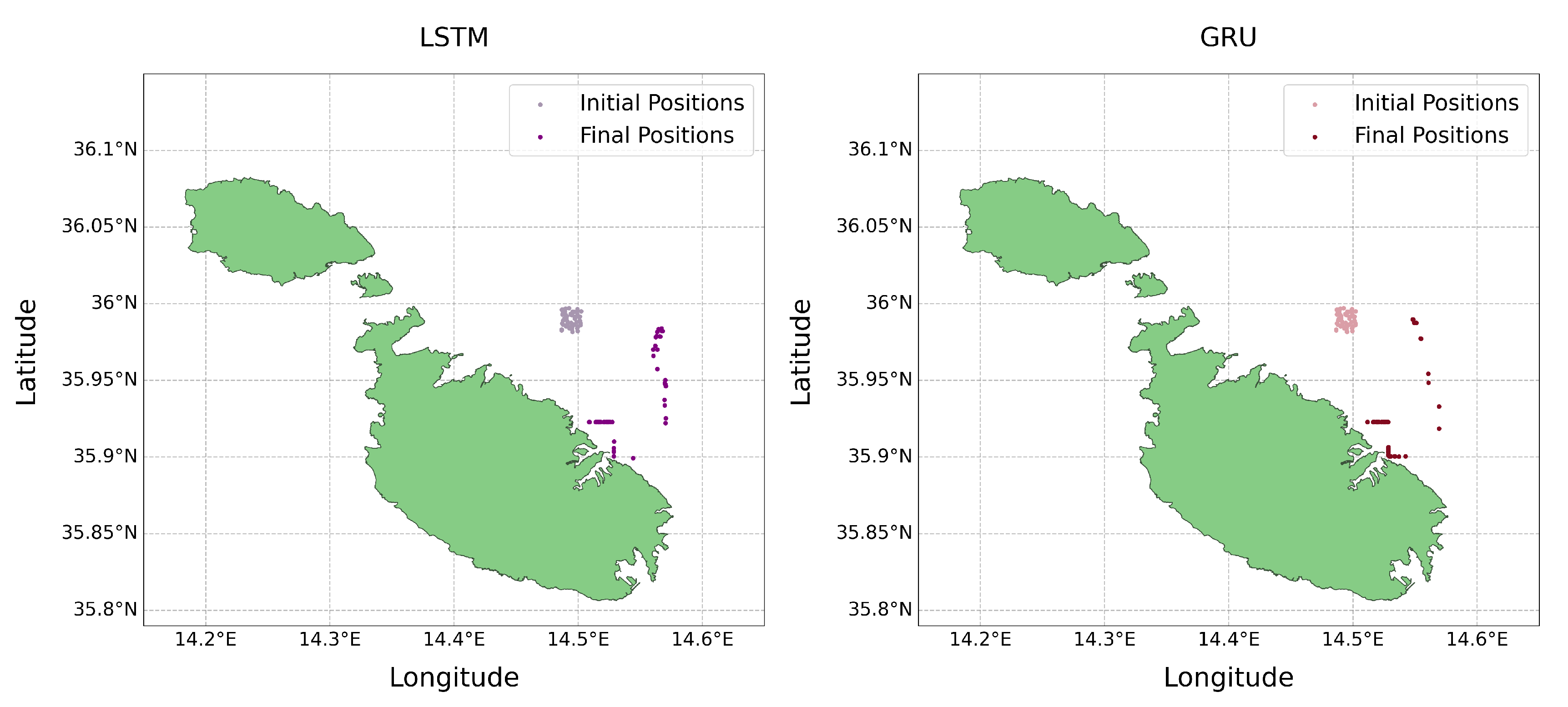
Finally, the Lagrangian simulations for both the LSTM and GRU models were executed and stored. The resulting particle movements and dispersion patterns were visualised. These visualisations (
Figure 11 and
Figure 19) allowed us to observe the surface debris movement predictions and facilitate the evaluation of the results produced by the LSTM and GRU models.
Figure 11.
LSTM and GRU initial vs final debris movement for Test 1 (4th August).
Figure 11.
LSTM and GRU initial vs final debris movement for Test 1 (4th August).
2.8. Evaluation Strategy
The original plan was to evaluate the Lagrangian framework by comparing dispersion patterns with drifter data, as done by van Sebille et al. [
33] and Aijaz et al. [
34]. However, due to the coastal proximity of our area of interest and the general practice of deploying drifters in open waters to avoid beaching, the drifter trajectory data was not available for our specific area. While this would be the ideal approach to assess the Lagrangian simulations, we were unable to do so due to the unavailability of drifter data. Instead, we focus on the analysis of LSTM and GRU model predictions. By adopting an approach similar to that of H. Yadav et al. [
35], where we use mean absolute error (MAE), mean squared error (MSE), and root mean squared error (RMSE) to asses their predictive accuracy. Furthermore, to ensure that our procedure generalises well, we also run it on the
Test 2 timeframe (in a different season) from the 1
th till the 3
th of November 2023 using the same trained models.
Given that our analysis includes 37 distinct models for both the u and v components, we computed the mean and standard deviation for each metric to facilitate a more comprehensive evaluation of the LSTM and GRU. During our analysis, we identified certain outliers within our results. To address this, we also calculated the average using the Interquartile range (IQR) focusing on the differences between the 75th and 25th percentiles for each metric thereby obtaining a more robust mean that excluded these outliers.
A geospatial evaluation of the LSTM and GRU models was motivated by the observation that each specific data point within the area of interest yields varied results. Initially, we generated a heat map (
Figure 7) to identify which model corresponds to each location and to quantify the amount of training data available for each model. Subsequently, we visualised the MAE values for the
u and
v components again using heat maps. The choice of MAE as a metric was deliberate, as it provides a straightforward and uniformly interpretable measure that treats all errors equivalently. These visualisations are instrumental in comparing the spatial accuracy of the models, highlighting areas where each model exhibited better or worse performance. These findings were then compared with the original heat map to discern patterns and discrepancies. This analysis is performed for the predictions corresponding to both
Test 1 and
Test 2.
Finally, we quantified the performance of the LSTM and GRU models across different regions, calculating the centroid, spread, and skewness for their respective Lagrangian simulation outputs. The measures include:
Mean, median, and standard deviation of centroids: we compute the geographical centroids of the merged predictions from both the LSTM and GRU models to assess the proximity of the final debris movement predictions generated by the two models. Smaller mean, median, and standard deviation values suggest a higher degree of consistency between the models’ predictions.
Spread of LSTM and GRU: the spatial spread is determined by calculating the standard deviation of distances from each model’s centroid. A lower standard deviation indicated a tighter clustering around the centroid, reflecting more consistent model performance across the area.
Longitudinal and latitudinal skewness of LSTM and GRU: to understand the directional tendencies of the models’ predictions, we calculate the skewness for the distribution of the prediction points’ longitude and latitude. A skewness close to zero indicates a symmetrical distribution of prediction errors, whereas a positive or negative skewness value points to a systematic bias in a particular direction.
3. Results
The primary objectives were to ascertain which model (LSTM or GRU) demonstrates superior performance and to evaluate the real-world similarity of the Lagrangian simulations generated using these models’ predictions. As previously noted, the framework was tested on two time periods. This was done to gauge the models’ consistency and reliability under varying seasonal conditions, offering a thorough analysis of their performance across different environmental dynamics.
3.1. LSTM vs GRU
In the initial experiment, we assessed the accuracy of the models in predicting SSC velocities by comparing the predicted results against actual historical values using MAE, MSE, and RMSE error metrics.
3.1.1. Error Metrics Results
The average error metrics for the 24-hour rolling predictions from all 37 models on
Test 1 are presented in
Table 1,
Table 2,
Table 3 and
Table 4 below.
The analysis of these results reveals insightful differences in model performance. For the u component, LSTM models demonstrate slightly lower MAE and RMSE, indicating better average accuracy and consistency, although GRU models show a marginally lower MSE. Conversely, for the v component, both models perform similarly with minimal variations across all metrics, which suggests a near-equivalent capability in handling this type of prediction. Further examination of the variability through standard deviation and IQR metrics shows that LSTM models have a lower standard deviation in the v component predictions, suggesting more consistent performance relative to GRU. Additionally, the smaller IQR for LSTM in both components implies that its predictions were more tightly clustered around the median, indicating less variability and more reliability. While both models performed well, LSTM offered marginally better performance, particularly for the u component, establishing it as the preferable model.
When it comes to the u component, both models displayed relatively high MAE, MSE, and RMSE, with LSTM showing lower metrics. The high standard deviations observed for both models suggest a significant presence of outliers, indicating some predictions were inaccurate. This is evident in the GRU u component, where the IQR is higher, suggesting a broader spread compared to LSTM, pointing to more frequent outliers in the GRU model. In contrast, the v component shows considerably higher error values for both models, with GRU again having higher values across all metrics. The standard deviations and IQR values are significantly larger in the v component for both models, again reinforcing the presence of outliers and indicating that predictions for the v component were generally less accurate and more variable. Overall, the LSTM model performed better than the GRU model, particularly in the v component, as evidenced by the lower error metrics and narrower IQR. Therefore, the more consistent performance of LSTM across both tests seems to suggest that it is the better model overall.
3.1.2. Discussion of Error Metrics Results
The analysis highlights that predictions for the
u component (east-west velocity) were generally more accurate than for the
v component (north-south velocity). This discrepancy can be attributed to the baseline alignment of radar systems, which are aligned along a north-south orientation, as depicted in
Figure 1. This potentially impacts the accuracy of
v component readings and inhibits the radar’s ability to capture detailed north-south data, consequently leading to less accurate predictions for the
v component. Moreover,
Test 1 conducted on the 4
th of August exhibited notably better results, characterised by lower error values and fewer outliers when compared to
Test 2 on the 4
th of November. This improvement is likely due to the August data being in close proximity to the final sequences of the test dataset, potentially leading to the models being better tuned to these conditions. Furthermore, the process of rolling forecasting, which bases predictions on preceding outputs, may lead to inaccuracies, particularly when initial predictions are derived from interpolated data. This method could inherently propagate errors, especially under conditions of notable missing data, as discussed in
Section 2.6.3. Such findings emphasise the necessity of considering temporal proximity and data integrity when assessing model performance. These phenomena and their implications on model performance will be explored further in the next section.
3.2. Geospatial Analysis
Another test focused on determining whether an increased volume of data correlates with enhanced predictive accuracy, whether data points closer to the coast, typically characterised by less data, yield poorer performance, and whether the time of year and seasonality of the data impact the results. The primary goal was to assess whether the geographical location of data points influences the accuracy of the predictive models. Additionally, we sought to compare the final Lagrangian simulations generated by both the LSTM and GRU models to evaluate their similarities in modelling sea surface debris.
3.2.1. A Hypothesis
As highlighted in
Section 2.6.1 and
Section 2.8, the dataset contains considerable missing data, with data points closer to the coast having more NaNs present, as evidenced in
Figure 7. This is corroborated by
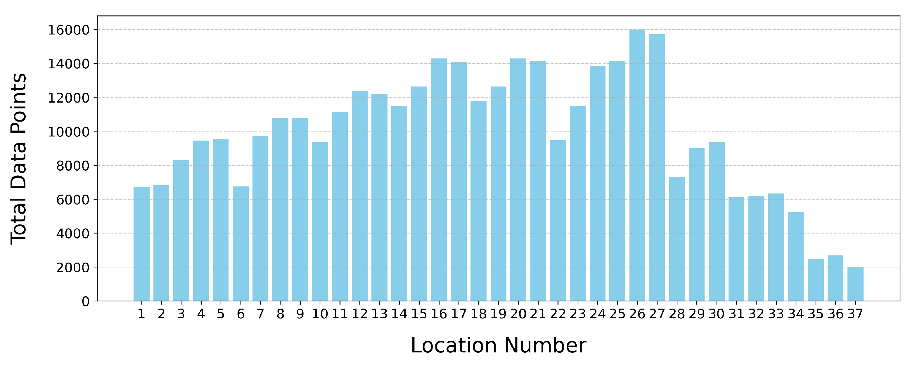
Figure 12, which illustrates how some data points have significantly less data available.
Figure 7 is instrumental in demonstrating the correlation between model performance and geographic location, thereby paving the way for a focused analysis on the impact of data availability at specific locations. Based on these observations, we formulated a hypothesis:
Hypothesis–Data points near the coast exhibit reduced data availability due to environmental and technical challenges that interfere with radar performance. This scarcity of data consequently impairs the accuracy of predictive models for SSC velocities near the coast. Specifically, it suggests that models predicting SSC at coastal locations perform less effectively compared to those further offshore, where radar data tends to be more complete.
We investigated the hypothesis by conducting a comparative analysis with the heat map in
Figure 7. This analysis helped us validate or refute our assumption regarding the influence of geographical location on model accuracy.
3.2.2. Heat Maps Results and Analysis
As discussed in
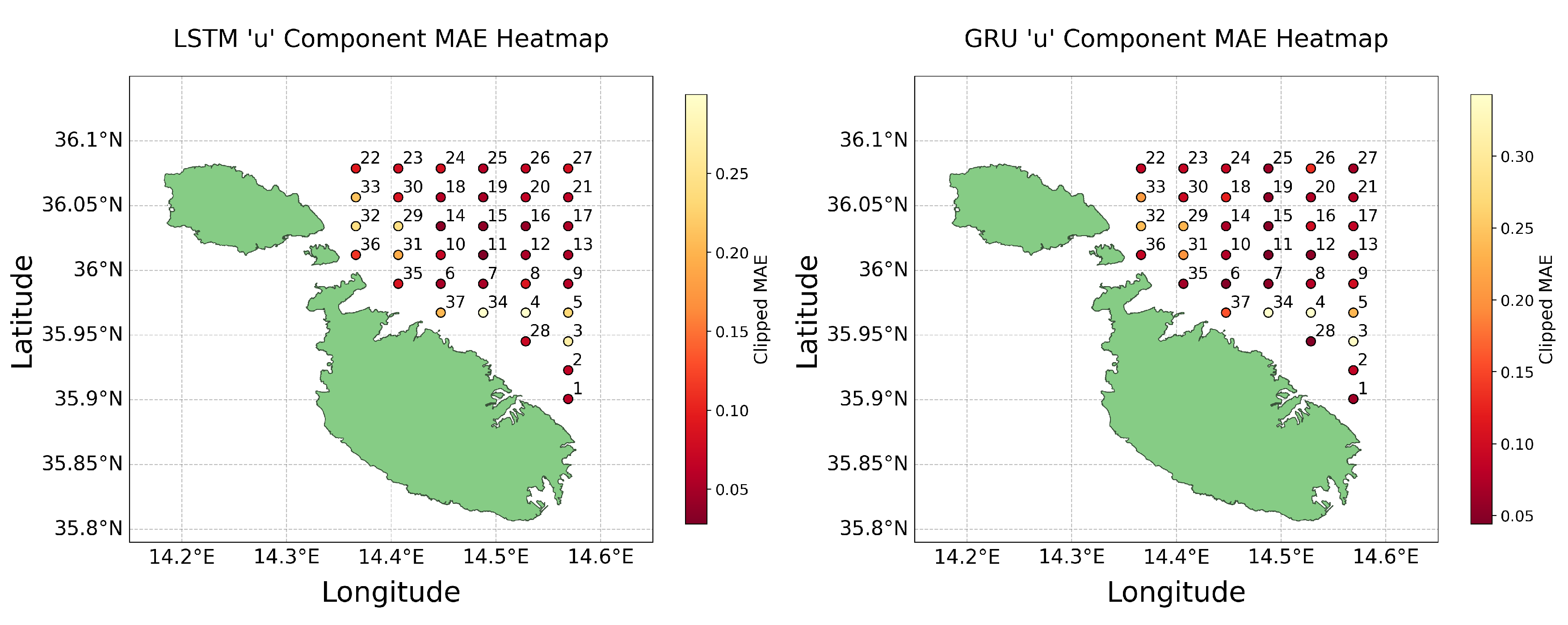
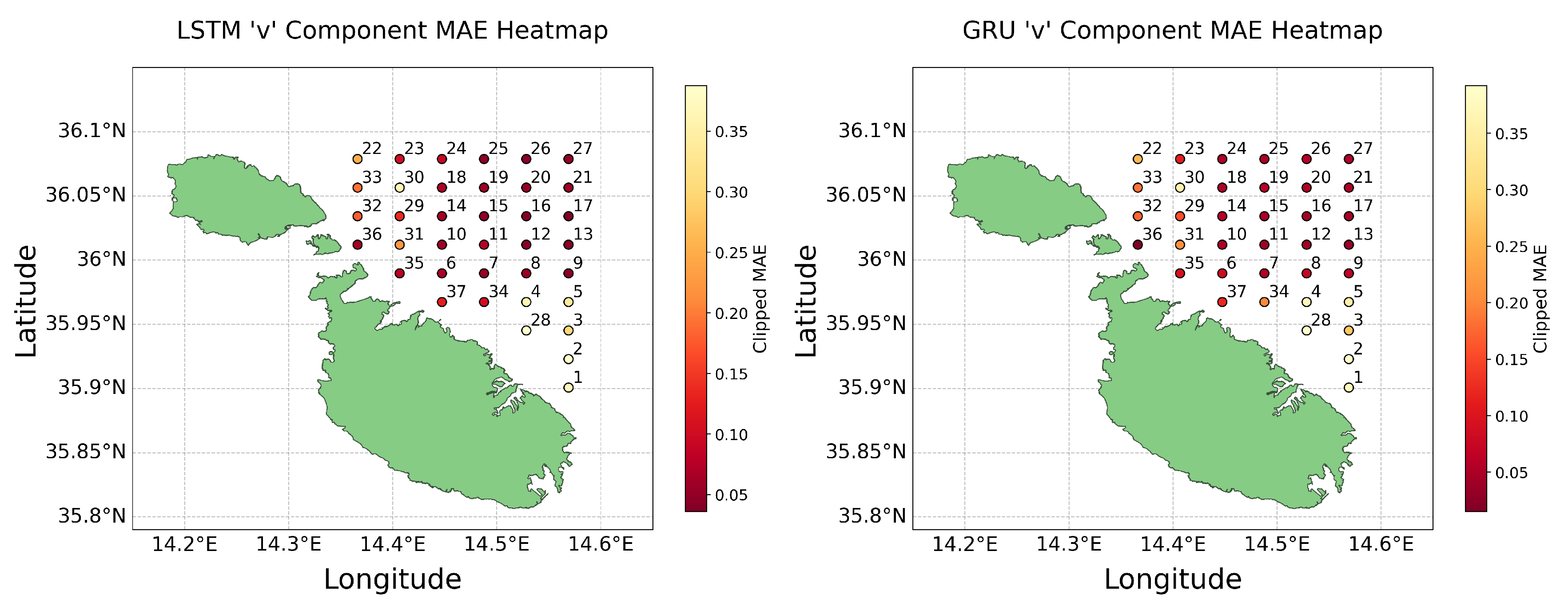
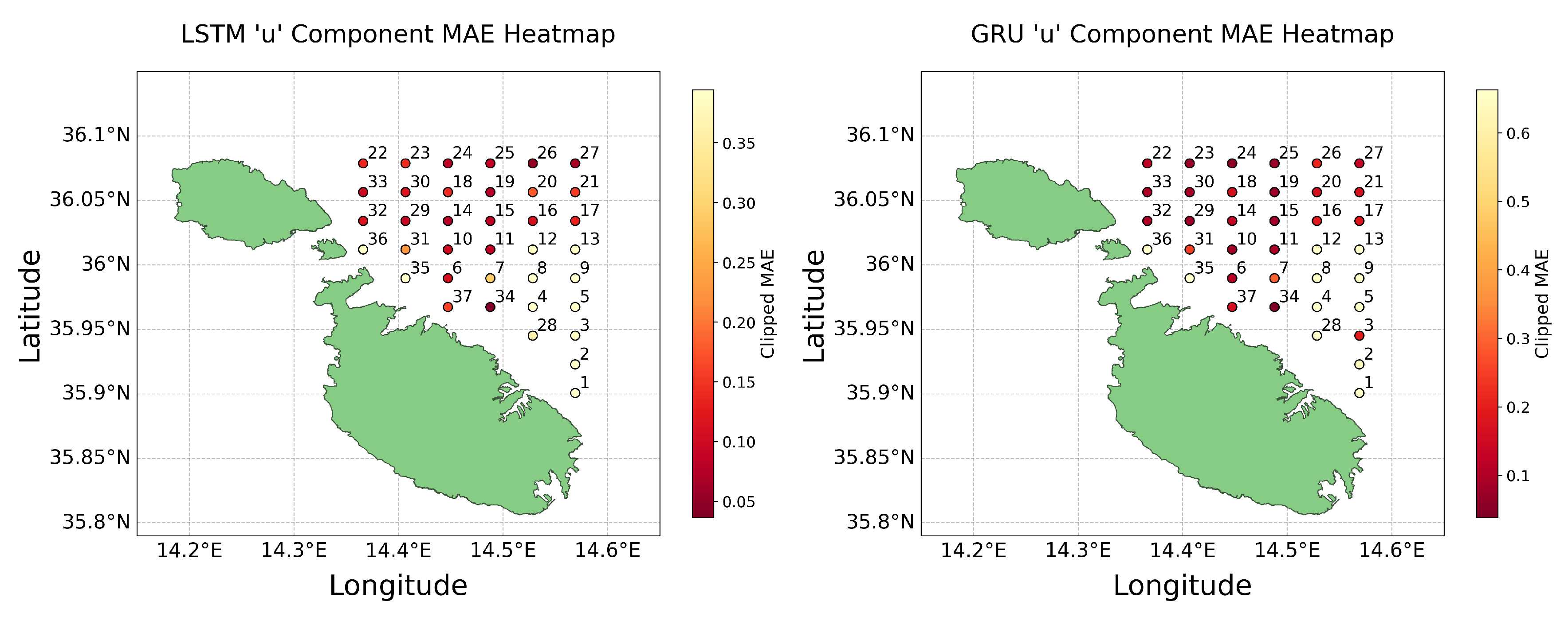
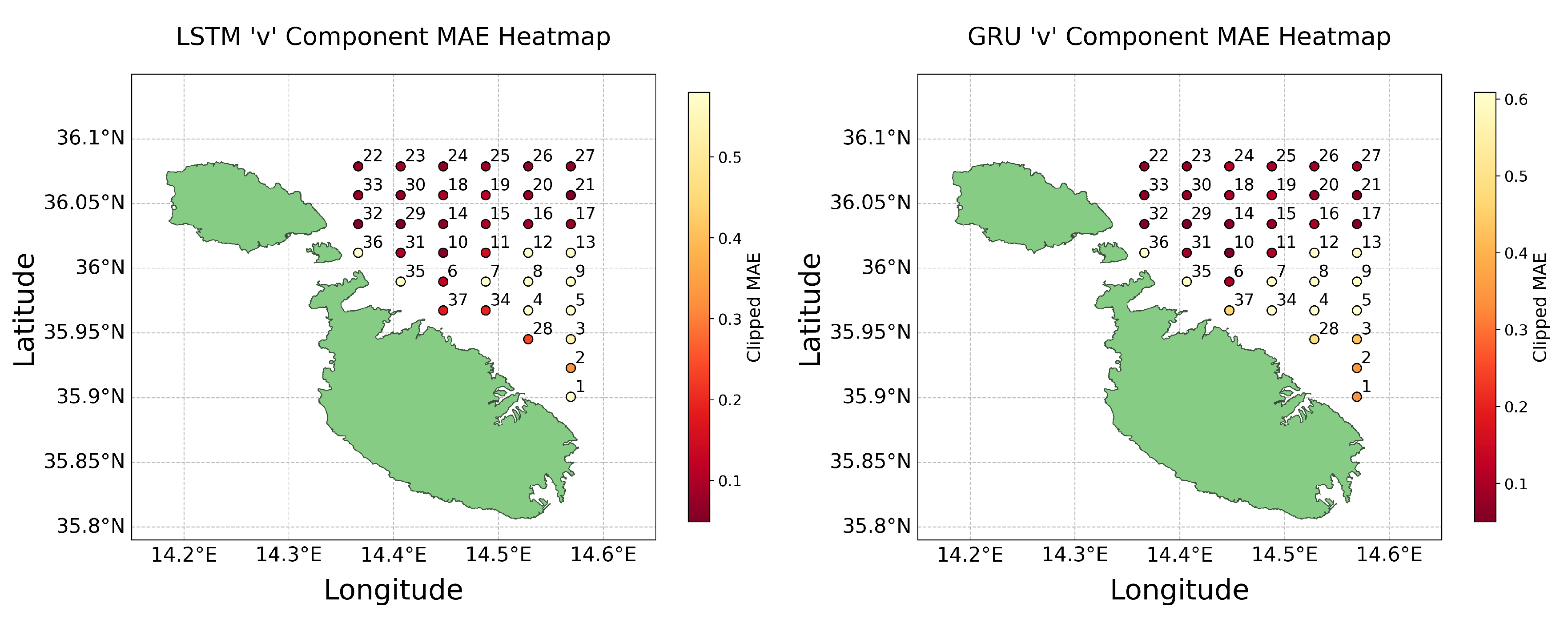
Section 2.8, heat maps were utilised to geospatially analyse the performance of the models, focusing on the MAE across all 37 models. These visualisations were crucial for testing the validity of our hypothesis regarding the impact of data availability on predictive accuracy near coastal areas. Heat maps for the MAE error metrics were produced for both the
u and
v components of both LSTM and GRU models, covering both the predictions made in
Test 1 and
Test 2. To enhance the clarity of these visualisations and minimise the influence of outliers, we applied a clipping method at the 95
th percentile of the data. This method effectively limited the range of data considered for colour scaling in the heat maps, allowing for more nuanced visual comparisons between most data points by excluding extreme outliers. The resultant heat maps for
Test 1 are displayed in
Figure 13 and
Figure 14 below.
These visualisations clarify that while models near the coast generally perform worse, presumably due to less data being available, there are notable exceptions where coastal predictions maintained good accuracy. This observation challenges the assumption that greater data volume directly correlates with higher predictive accuracy. Instead, it suggests that the models’ capabilities to handle noise and extract meaningful patterns from sparse data can significantly impact their effectiveness. Furthermore, the differential accuracy between the u and v components highlights the complexity of environmental factors and model sensitivities, which contribute to a diverse spectrum of outcomes that are not solely determined by the amount of data available.
Comparing the results obtained by the two tests reveals a stark contrast; predictions for August are markedly more accurate, underscoring the potential impact of seasonal variations. The outliers observed in Test 1 are inconsistent with those of Test 2, highlighting the temporal variability of missing data and its non-uniform impact across different points and times. It becomes evident that no consistent pattern exists, thus challenging any definitive conclusions. While certain models excel in predicting the u component, their performance diminishes when applied to the v component. These observations attest to the intricate dynamics at play in predictive modelling, where factors like the models’ ability to manage noise and the inherent directional properties of data lead to outcomes where less data does not always result in less accuracy. Therefore, these findings not only challenge but effectively refute the hypothesis.
3.2.3. Comparison of Lagrangian Simulations
In the final component of the evaluation framework, the performance similarities between the LSTM and GRU models was assesed by analysing centroids, spreads, and skewness within the respective Lagrangian simulation outputs. The findings for
Test 1 are shown in
Figure 17.
In this case, the average centroid distances for the LSTM and GRU models were around 2 km, suggesting both models achieved markedly different geographical accuracy. The standard deviation of these distances was 1.54 km, indicating a moderate spread around the centroids. However, the GRU model demonstrated a more compact spread of 0.54 km compared to the LSTM’s 1.81 km, suggesting GRU’s predictions were more tightly grouped. The skewness metrics showed a mild eastward and southward bias in the LSTM predictions, whereas the GRU exhibited a stronger westward bias and a slight northward tendency, highlighting directional tendencies in their prediction patterns. Next, the results for
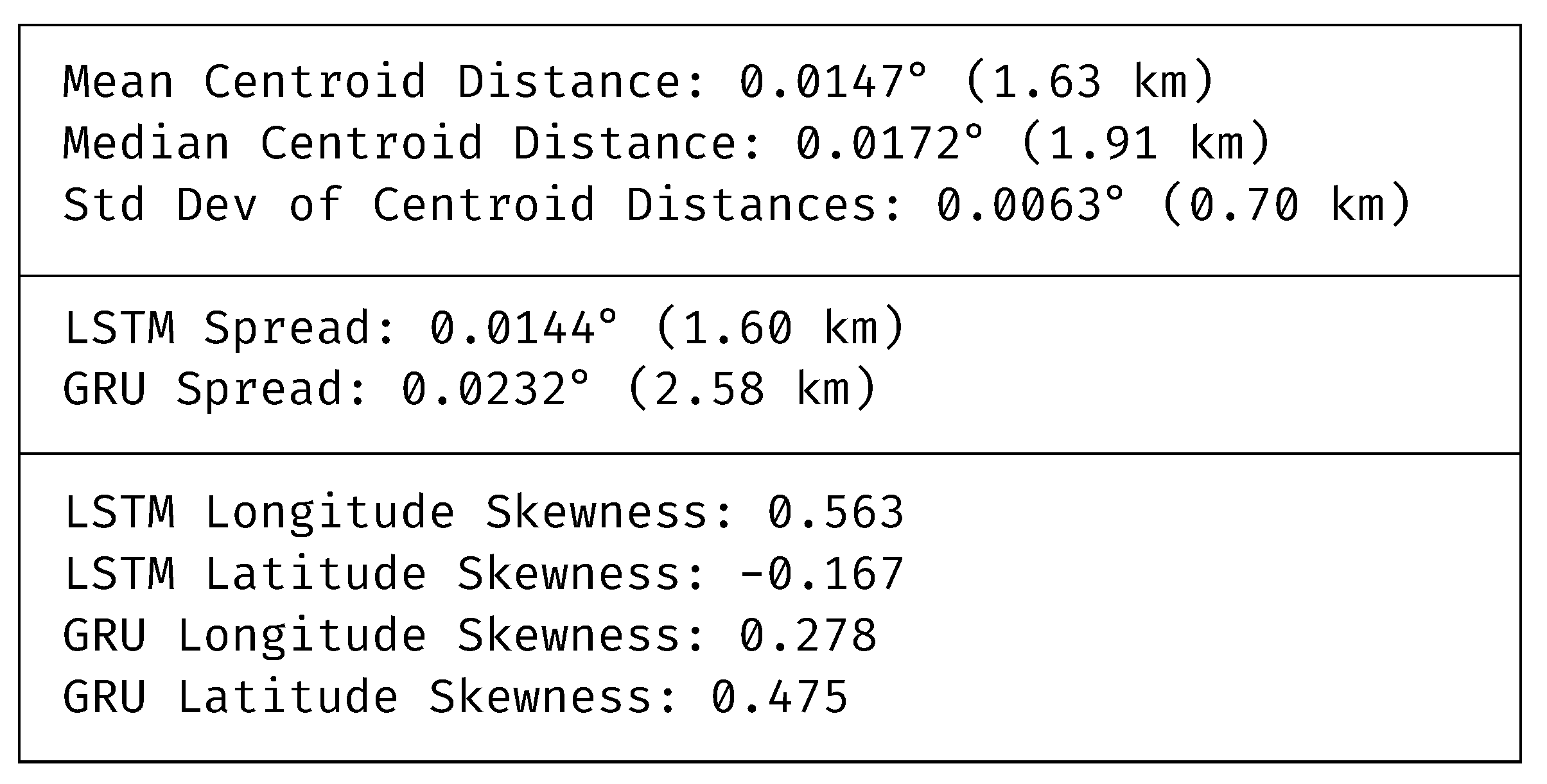
Test 2 are shown in
Figure 18.
The results from the second test showed improvements in clustering, with mean and median centroid distances reduced to approximately 1.63 km and 1.91 km, respectively. This reduction, coupled with a decreased standard deviation of 0.70 km, suggests enhanced prediction accuracy and consistency for this period. Interestingly, LSTM showed a more consistent spread of 1.60 km, whereas GRU’s predictions were more dispersed, with a spread of 2.58 km. Skewness values also shifted, indicating changes in predictive behaviour that might be influenced by different environmental conditions or model sensitivities to the input data at that time.
Overall, the analyses highlight that the LSTMs generally offer more consistent and reliable performance, marked by less variability in spread and skewness compared to GRUs. While GRUs seemed to adjust its performance based on different conditions, suggesting a possible sensitivity to seasonal or environmental changes, the LSTMs maintained steadiness across the evaluated metrics. This consistent performance makes LSTMs the more suitable model for this application.
3.2.4. Comparison of Final Lagrangian Visualisations
The visual comparisons between
Figure 11 and
Figure 19 indicate notable differences in the outcomes of the LSTM and GRU simulations. Specifically, the August simulations (
Figure 11) reveal distinct disparities in the final particle locations between the LSTM and GRU models. Conversely, the November simulations (
Figure 19) display a high degree of similarity. This observation lends support to findings from our previous observations in
Section 3.2.3, where the November results demonstrated greater alignment between the models when compared to August. Such disparities point out the variable nature of these predictions and highlight the complex interplay of various factors that significantly impact the accuracy and consistency of the final outcomes. This variability is illustrative of the inherent challenges in modelling time series data, where slight variations in input or parameters can lead to markedly different predictions.
Figure 19.
LSTM and LSTM initial vs final debris movement for Test 2 (4th November).
Figure 19.
LSTM and LSTM initial vs final debris movement for Test 2 (4th November).
4. Discussion and Conclusions
In this study, an integrated system that combines ML models with a physics-based Lagrangian framework to forecast the movement and dispersion of sea surface debris around Malta was proposed. The results demonstrate the capability of the system to make accurate 24-hour predictions and dynamically visualise the trajectory of marine debris. Through a comparative evaluation, it was determined that the LSTM model outperforms the GRU model in predicting SSC velocities, evidenced by better performance in error metrics such as mean absolute error (MAE), mean squared error (MSE), and root mean squared error (RMSE). These findings validate the effectiveness of the integrated approach and demonstrate its potential to enhance marine conservation efforts.
The analysis consists of an evaluation of error metrics and geospatial behaviour, which together provide a robust evaluation of the effectiveness of the models and the corresponding practical applicability. The findings indicate that LSTM provides more consistent and reliable predictions, establishing it as the preferred model when considering the performance of both components across diverse seasonal and environmental conditions. The geospatial analysis further corroborated these findings, showing that the LSTM generally maintains more consistent performance metrics, such as spread and skewness, when compared to the GRU. This consistency was evident despite the seasonal variations between the two dates, highlighting LSTM’s robustness across different predictive scenarios.
Furthermore, this analysis does not consistently support the hypothesis that proximity to the coast and reduced data availability significantly degraded model performance. While coastal data points generally showed less accuracy, this was not universally the case. Some predictions maintained good accuracy, suggesting that other factors, such as the capacity of the models to handle sparse data and environmental noise, play a critical role in prediction outcomes. Therefore, the findings do not support the hypothesis that less data inherently results in poorer model performance.
Throughout this study, several challenges and limitations were encountered. The primary challenge was the presence of missing data, particularly near coastal areas, which likely affected the precision of our predictive models. Moreover, the geographical area of interest was limited, potentially constraining the broader applicability of our findings. The final limitation was the inability to empirically validate the Lagrangian model due to the absence of drifter data within the chosen area.
Integrating additional weather parameters such as wind and wave action into the models to enhance the predictions, is left as future work. Additionally, the framework can be adapted to various applications, including jellyfish and plankton movements, search and rescue operations, as well as oil spill trajectory simulations. Further enhancements in predictive accuracy could be achieved by implementing ensemble learning methods, as evidenced by the research of B. Naderalvojoud and T. Hernandez-Boussard [
36], and by integrating more sophisticated models such as transformers [
37]. Expanding the area of interest could provide a more comprehensive understanding of marine debris dynamics, while also enabling the evaluation of the Lagrangian model using historical drifter data. Implementing a model specifically designed to predict and fill missing values within the datasets could enhance the accuracy of predictions and improve visualisations. Finally, developing a front-end to display future predictions with enhanced visualisations would make the research more accessible, allowing interaction with the data in real-time, and fostering greater engagement and understanding of the capabilities of the model and environmental implications.
The primary goal of this work was to design and develop a predictive modelling system that leverages the strengths of AI techniques integrated with a physics-based model to predict and visualise the dispersion of sea surface debris around the coastal waters of Malta. The LSTM model was found to outperform the GRU model in terms of prediction accuracy. Overall, this work is a comprehensive system that enhances marine conservation efforts by providing actionable insights for effective cleanup operations and simultaneously informing strategies for long-term marine conservation around the coast of Malta.
Author Contributions
Conceptualisation (MD/AG/KG); Methodology (MD/KG); Investigation (MD/KG); Dataset (AG); Evaluation (MD); Analysis (MD/KG); Writing – Original Draft (MD/KG); Writing – Review and Editing (MD/AG/KG); Project Administration (KG). All authors have read and agreed to the published version of the manuscript.
Funding
This research received no external funding.
Data Availability Statement
Conflicts of Interest
The authors declare no conflict of interest.
Abbreviations
The following abbreviations are used in this manuscript:
| AI |
Artificial Intelligence |
| ANN |
Artificial Neural Networks |
| GRU |
Gated Recurrent Unit |
| IQR |
Interquartile Range |
| LSTM |
Long Short-Term Memory |
| MAE |
Mean Absolute Error |
| ML |
Machine Learning |
| MSE |
Mean Squared Error |
| NetCDF |
Network Common Data Form |
| NaN |
Not a Number |
| RNN |
Recurrent Neural Network |
| RMSE |
Root Mean Squared Error |
| CSV |
Comma-separated Value |
| SSC |
Sea Surface Currents |
References
- Kehl, C.; Nooteboom, P.D.; Kaandorp, M.L.A.; van Sebille, E. Efficiently simulating Lagrangian particles in large-scale ocean flows — Data structures and their impact on geophysical applications. Computers and Geosciences 2023, 175, 105322. [Google Scholar] [CrossRef]
- Suaria, G.; Aliani, S. Floating debris in the Mediterranean Sea. Marine pollution bulletin 2014, 86, 494–504. [Google Scholar] [CrossRef] [PubMed]
- Compa, M.; Alomar, C.; Wilcox, C.; van Sebille, E.; Lebreton, L.; Hardesty, B.D.; Deudero, S. Risk assessment of plastic pollution on marine diversity in the Mediterranean Sea. Science of The Total Environment 2019, 678, 188–196. [Google Scholar] [CrossRef] [PubMed]
- Laist, D.W. Impacts of Marine Debris: Entanglement of Marine Life in Marine Debris Including a Comprehensive List of Species with Entanglement and Ingestion Records; Marine Debris: Sources, Impacts, and Solutions, Springer New York: New York, NY, 1997; pp. 99–139. [CrossRef]
- Rochman, C.M.; Browne, M.A.; Underwood, A.J.; van Franeker, J.A.; Thompson, R.C.; Amaral-Zettler, L.A. The ecological impacts of marine debris: unraveling the demonstrated evidence from what is perceived. Ecology 2016, 97, 302–312. [Google Scholar] [CrossRef] [PubMed]
- Agamuthu, P.; Mehran, S.B.; Norkhairah, A.; Norkhairiyah, A. Marine debris: A review of impacts and global initiatives. Waste management and research : the journal of the International Solid Wastes and Public Cleansing Association, ISWA 2019, 37, 987–1002. [Google Scholar] [CrossRef]
- Mansui, J.; Darmon, G.; Ballerini, T.; van Canneyt, O.; Ourmieres, Y.; Miaud, C. Predicting marine litter accumulation patterns in the Mediterranean basin: Spatio-temporal variability and comparison with empirical data. Progress in Oceanography 2020, 182, 102268. [Google Scholar] [CrossRef]
- Ryan, P.G. A Brief History of Marine Litter Research; Marine Anthropogenic Litter, Springer International Publishing: Cham, 2015; pp. 1–25. [CrossRef]
- Harlan, J.; Terrill, E.; Hazard, L.; Keen, C.; Barrick, D.; Whelan, C.; Howden, S.; Kohut, J. The Integrated Ocean Observing System High-Frequency Radar Network: Status and Local, Regional, and National Applications. Marine Technology Society journal 2010, 44, 122–132. [Google Scholar] [CrossRef]
- UNIDATA | NETCDF. https://www.unidata.ucar.edu/software/netcdf/. Accessed: 14-03-2024.
- van Sebille, E.; Griffies, S.M.; Abernathey, R.; Adams, T.P.; Berloff, P.; Biastoch, A.; Blanke, B.; Chassignet, E.P.; Cheng, Y.; Cotter, C.J.; et al. Lagrangian ocean analysis: Fundamentals and practices. Ocean Modelling 2018, 121, 49–75. [Google Scholar] [CrossRef]
- Lonin, S.A. Lagrangian model for oil spill diffusion at sea. Spill Science and Technology Bulletin 1999, 5, 331–336. [Google Scholar] [CrossRef]
- Lebreton, L.C.M.; Greer, S.D.; Borrero, J.C. Numerical modelling of floating debris in the world’s oceans. Marine pollution bulletin 2012, 64, 653–661. [Google Scholar] [CrossRef]
- Dawson, M.N.; Gupta, A.S.; England, M.H. Coupled biophysical global ocean model and molecular genetic analyses identify multiple introductions of cryptogenic species. Proceedings of the National Academy of Sciences 2005, 102, 11968–11973. [Google Scholar] [CrossRef] [PubMed]
- Hertwig, D.; Burgin, L.; Gan, C.; Hort, M.; Jones, A.; Shaw, F.; Witham, C.; Zhang, K. Development and demonstration of a Lagrangian dispersion modeling system for real-time prediction of smoke haze pollution from biomass burning in Southeast Asia. Journal of geophysical research. Atmospheres 2015, 120, 12605–12630. [Google Scholar] [CrossRef]
- Williams, R.G.; Follows, M.J. Ocean Dynamics and the Carbon Cycle: Principles and Mechanisms; Cambridge University Press: Cambridge, 2011. [Google Scholar] [CrossRef]
- OceanParcels. https://oceanparcels.org. Accessed: 2024-03-27.
- PyGNOME. https://gnome.orr.noaa.gov/doc/pygnome/index.html. Accessed: 2024-03-27.
- Pisso, I.; Sollum, E.; Grythe, H.; Kristiansen, N.I.; Cassiani, M.; Eckhardt, S.; Arnold, D.; Morton, D.; Thompson, R.L.; Zwaaftink, C.G.; et al. The Lagrangian particle dispersion model FLEXPART version 10.4. 2019. [Google Scholar] [CrossRef]
- Adhikari, R.; Agrawal, R.K. An Introductory Study on Time Series Modeling and Forecasting. ArXiv 2013. [Google Scholar]
- Raicharoen, T.; Lursinsap, C.; Sanguanbhokai, P. Application of critical support vector machine to time series prediction. 2003, Vol. 5, p. V. [CrossRef]
- Raksha, S.; Graceline, J.S.; Anbarasi, J.; Prasanna, M.; Kamaleshkumar, S. Weather Forecasting Framework for Time Series Data using Intelligent Learning Models. 2021, pp. 783–787. [CrossRef]
- Chatterjee, A.; Bhowmick, H.; Sen, J. Stock Price Prediction Using Time Series, Econometric, Machine Learning, and Deep Learning Models. 2021, pp. 289–296. [CrossRef]
- Wang, P.; Gurmani, S.H.; Tao, Z.; Liu, J.; Chen, H. Interval time series forecasting: A systematic literature review. Journal of forecasting 2024, 43, 249–285. [Google Scholar] [CrossRef]
- Jadon, S.; Milczek, J.; Patankar, A. Challenges and approaches to time-series forecasting in data center telemetry: A Survey. Technical report, Cornell University Library, arXiv.org, 2021. [CrossRef]
- Alsharef, A.; Sonia. ; Kumar, K.; Iwendi, C. Time Series Data Modeling Using Advanced Machine Learning and AutoML. Sustainability 2022, 14. [Google Scholar] [CrossRef]
- Hamayel, M.J.; Owda, A.Y. A Novel Cryptocurrency Price Prediction Model Using GRU, LSTM and bi-LSTM Machine Learning Algorithms. AI 2021, 2, 496. [Google Scholar] [CrossRef]
- Yamak, P.T.; Yujian, L.; Gadosey, P.K. A Comparison between ARIMA, LSTM, and GRU for Time Series Forecasting, 2020. [CrossRef]
- Eriksen, M.; Lebreton, L.C.M.; Carson, H.S.; Thiel, M.; Moore, C.J.; Borerro, J.C.; Galgani, F.; Ryan, P.G.; Reisser, J. Plastic Pollution in the World’s Oceans: More than 5 Trillion Plastic Pieces Weighing over 250,000 Tons Afloat at Sea. PloS one 2014, 9, e111913. [Google Scholar] [CrossRef] [PubMed]
- Ali, A.M.; Zhuang, H.; VanZwieten, J.; Ibrahim, A.K.; Chérubin, L. A Deep Learning Model for Forecasting Velocity Structures of the Loop Current System in the Gulf of Mexico. Forecasting 2021, 3, 953. [Google Scholar] [CrossRef]
- Zulfa, I.I.; Novitasari, D.C.R.; Setiawan, F.; Fanani, A.; Hafiyusholeh, M. Prediction of Sea Surface Current Velocity and Direction Using LSTM. IJEIS (Indonesian Journal of Electronics and Instrumentation Systems) (Online) 2021, 11, 93–102. [Google Scholar] [CrossRef]
- Choi, H.M.; Kim, M.K.; Yang, H. Deep-learning model for sea surface temperature prediction near the Korean Peninsula. Deep Sea Research Part II: Topical Studies in Oceanography 2023, 208, 105262. [Google Scholar] [CrossRef]
- van Sebille, E.; Aliani, S.; Law, K.L.; Maximenko, N.; Alsina, J.M.; Bagaev, A.; Bergmann, M.; Chapron, B.; Chubarenko, I.; Cózar, A.; et al. The physical oceanography of the transport of floating marine debris. Environmental research letters 2020, 15, 23003–32. [Google Scholar] [CrossRef]
- Aijaz, S.; Colberg, F.; Brassington, G.B. Lagrangian and Eulerian modelling of river plumes in the Great Barrier Reef system, Australia. Ocean Modelling 2024, 188, 102310. [Google Scholar] [CrossRef]
- Yadav, H.; Thakkar, A. NOA-LSTM: An efficient LSTM cell architecture for time series forecasting. Expert Systems with Applications 2024, 238, 122333. [Google Scholar] [CrossRef]
- Naderalvojoud, B.; Hernandez-Boussard, T. Improving machine learning with ensemble learning on observational healthcare data. AMIA Annu Symp Proc 2024, 2023, 521–529. [Google Scholar] [PubMed]
- Vaswani, A.; Shazeer, N.; Parmar, N.; Uszkoreit, J.; Jones, L.; Gomez, A.N.; Kaiser, L.u.; Polosukhin, I. Attention is All you Need. Advances in Neural Information Processing Systems; Guyon, I.; Luxburg, U.V.; Bengio, S.; Wallach, H.; Fergus, R.; Vishwanathan, S.; Garnett, R., Eds. Curran Associates, Inc., 2017, Vol. 30.
| 1 |
|
| 2 |
|
| 3 |
|
| 4 |
|
| 5 |
This is distinct from the case where NaNs were ignored ( Section 2.5) |
Figure 1.
High-frequency radar locations highlighted in orange.
Figure 1.
High-frequency radar locations highlighted in orange.
Figure 2.
Locations of radar data points.
Figure 2.
Locations of radar data points.
Figure 3.
Land-sea mask of Malta.
Figure 3.
Land-sea mask of Malta.
Figure 4.
Location of initial particles showing a cluster of debris.
Figure 4.
Location of initial particles showing a cluster of debris.
Figure 5.
All data points and selected area of interest.
Figure 5.
All data points and selected area of interest.
Figure 6.
Filtered points within area of interest.
Figure 6.
Filtered points within area of interest.
Figure 7.
Amount of data points per coordinate pair.
Figure 7.
Amount of data points per coordinate pair.
Figure 8.
Actual vs predicted values on the test set.
Figure 8.
Actual vs predicted values on the test set.
Figure 9.
The process of a rolling forecast.
Figure 9.
The process of a rolling forecast.
Figure 12.
Histogram of data points by location number.
Figure 12.
Histogram of data points by location number.
Figure 13.
u component MAE heat maps for Test 1 (4th August).
Figure 13.
u component MAE heat maps for Test 1 (4th August).
Figure 14.
v component MAE heat maps for Test 1 (4th August).
Figure 14.
v component MAE heat maps for Test 1 (4th August).
Figure 15.
u component MAE heat maps for Test 2 (4th November).
Figure 15.
u component MAE heat maps for Test 2 (4th November).
Figure 16.
v component MAE heat maps for Test 2 (4th November).
Figure 16.
v component MAE heat maps for Test 2 (4th November).
Figure 17.
LSTM vs GRU comparison on Lagrangian simulations for Test 1 (4th August).
Figure 17.
LSTM vs GRU comparison on Lagrangian simulations for Test 1 (4th August).
Figure 18.
LSTM vs GRU comparison on Lagrangian simulations for Test 2 (4th November).
Figure 18.
LSTM vs GRU comparison on Lagrangian simulations for Test 2 (4th November).
Table 1.
LSTM u average error metrics for Test 1 (4th August).
Table 1.
LSTM u average error metrics for Test 1 (4th August).
| Metric |
Mean |
Std Dev |
IQR |
| MAE |
0.141 |
0.226 |
0.058 |
| MSE |
0.116 |
0.513 |
0.010 |
| RMSE |
0.179 |
0.291 |
0.053 |
Table 2.
LSTM v average error metrics for Test 1 (4th August).
Table 2.
LSTM v average error metrics for Test 1 (4th August).
| Metric |
Mean |
Std Dev |
IQR |
| MAE |
0.144 |
0.134 |
0.141 |
| MSE |
0.064 |
0.109 |
0.073 |
| RMSE |
0.183 |
0.175 |
0.212 |
Table 3.
GRU u average error metrics for Test 1 (4th August).
Table 3.
GRU u average error metrics for Test 1 (4th August).
| Metric |
Mean |
Std Dev |
IQR |
| MAE |
0.148 |
0.222 |
0.067 |
| MSE |
0.116 |
0.503 |
0.016 |
| RMSE |
0.187 |
0.285 |
0.070 |
Table 4.
GRU v average error metrics for Test 1 (4th August).
Table 4.
GRU v average error metrics for Test 1 (4th August).
| Metric |
Mean |
Std Dev |
IQR |
| MAE |
0.145 |
0.138 |
0.149 |
| MSE |
0.066 |
0.112 |
0.066 |
| RMSE |
0.184 |
0.179 |
0.202 |
Table 5.
LSTM u average error metrics for Test 2 (4th November).
Table 5.
LSTM u average error metrics for Test 2 (4th November).
| Metric |
Mean |
Std Dev |
IQR |
| MAE |
1.031 |
2.118 |
0.299 |
| MSE |
14.765 |
40.758 |
0.243 |
| RMSE |
1.634 |
3.478 |
0.397 |
Table 6.
LSTM v average error metrics for Test 2 (4th November).
Table 6.
LSTM v average error metrics for Test 2 (4th November).
| Metric |
Mean |
Std Dev |
IQR |
| MAE |
2.622 |
5.507 |
0.506 |
| MSE |
97.858 |
253.429 |
0.860 |
| RMSE |
4.239 |
8.938 |
0.844 |
Table 7.
GRU u average error metrics for Test 2 (4th November).
Table 7.
GRU u average error metrics for Test 2 (4th November).
| Metric |
Mean |
Std Dev |
IQR |
| MAE |
1.051 |
2.112 |
0.568 |
| MSE |
14.772 |
40.773 |
0.466 |
| RMSE |
1.651 |
3.471 |
0.586 |
Table 8.
GRU v average error metrics for Test 2 (4th November).
Table 8.
GRU v average error metrics for Test 2 (4th November).
| Metric |
Mean |
Std Dev |
IQR |
| MAE |
2.653 |
5.502 |
0.537 |
| MSE |
97.980 |
253.623 |
1.144 |
| RMSE |
4.268 |
8.931 |
0.991 |
|
Disclaimer/Publisher’s Note: The statements, opinions and data contained in all publications are solely those of the individual author(s) and contributor(s) and not of MDPI and/or the editor(s). MDPI and/or the editor(s) disclaim responsibility for any injury to people or property resulting from any ideas, methods, instructions or products referred to in the content. |
© 2024 by the authors. Licensee MDPI, Basel, Switzerland. This article is an open access article distributed under the terms and conditions of the Creative Commons Attribution (CC BY) license (http://creativecommons.org/licenses/by/4.0/).
