Game Theory for Predicting Stocks’ Closing Prices

Preprint

Article

Game Theory for Predicting Stocks’ Closing Prices

Altmetrics

Downloads

Views

Comments

A peer-reviewed article of this preprint also exists.

João Costa Freitas^*

Alberto Adrego Pinto^*,

Óscar Felgueiras^*

João Costa Freitas^*

Alberto Adrego Pinto^*,

Óscar Felgueiras^*

This version is not peer-reviewed

Submitted:

19 July 2024

Posted:

22 July 2024

You are already at the latest version

Alerts

Abstract

We model the financial markets as a game and make predictions using Markov chains estimators. We extract the possible patterns displayed by the financial markets, define a game where one of the players is the speculator, whose strategies depend on his/hers risk-to-reward preferences, and the market is the other player, whose strategies are the previously observed patterns. Then we estimate the market’s mixed probabilities by defining Markov chains and utilizing its transitions matrices. Afterwards, we use these probabilities to determine which is the optimal strategy for the speculator. Finally, we apply these models to real-time market data to determine its feasibility. After all, we obtained a model for the financial markets that has an outstanding performance in terms of accuracy and profitability.

Keywords:

Subject: Computer Science and Mathematics - Applied Mathematics

1. Introduction

In this article, we will present and apply methods specifically designed to model the financial market, but, before starting to discuss the models, we need to make a brief introduction to the data that we will be working with.

Our data consists on financial asset prices from several stock exchanges, with special attention to the New York Stock Exchange, the London Stock Exchange and the Lisbon Stock Exchange. Also, we focused on stock and forex (foreign exchange market) prices, because these present higher volatility and volume (i.e., more trades), and the data related to these assets is easier to obtain. Here, volatility is a statistical measure of the dispersion of returns for a given financial asset. It is often measured as either the standard deviation or variance between returns from that same asset.

Moving further we will often use the terms "stock exchange" and "financial market" interchangeably, but they slightly differ. The term "financial market" broadly refers to any marketplace where the trading of securities occurs, including the stock market, bond market, forex market, and derivatives market, among others, whilst the "stock exchange" is a facility where stockbrokers and traders can buy and sell securities, such as shares of stock, bonds and other financial instruments. However, whenever we refer to the financial market we will be referring to the stock exchange.

The data was retrieved from Yahoo Finance, AlphaVantage and WorldTradingData, but it can be found at https://www.kaggle.com/jfcf0802/daily-and-intraday-stock-data.

We will study daily closing prices, that is, the price of the asset at the end of the day, and also intraday closing prices, i.e., the prices of the asset at the end of each minute. Also, we will look into several assets within multiple stock exchanges. Specifically, we will analyze:

3 theoretical datasets with 1000 observations;
100 datasets with 1000 observations of stocks’ daily closing prices from several stock exchanges;
100 datasets with 1000 observations of stocks’ intraday closing prices from several stock exchanges.

Hence, we will obtain all kinds of data, with different characteristics and statistical properties. Moreover, since we cannot access the assets’ future prices, we will split the datasets between training and test sets. All the analyzed datasets have 1000 observations and

20 %

of these will be part of the test sets. This is done so that we can apply our models to the training set and "compare" their predictions with the test set’s values.

To exemplify, consider the following datasets from the New York Stock Exchange (plots 1 and 2) and from the Lisbon Stock Exchange (plots 3 and 4):

Measuring past price changes to determine their dispersion should yield a probabilistic result. Additionally, price changes, in stock prices (or in any other financial instruments), usually pattern themselves in a normal distribution (for further details see [1,2,3] and/or [4]), which is the familiar bell-shaped curve (for further details see, for example, [5]). There are numerous different ways to determine the probability function for a financial instrument. Also, price changes can be measured and quantified empirically, either by the percent change in the instrument’s value over specified time intervals or by the change in the logarithm of the price over the time intervals.

Oftentimes when you’re thinking in terms of compounding percent changes, the mathematically cleaner concept is to think in terms of log differences. When you’re repeatedly multiplying terms together, usually, it’s more convenient to work in logs and add terms together. So, let’s say our wealth at time T is given by:

W_{T} = \prod_{t = 1}^{T} (1 + R_{t}) \Leftrightarrow log W_{T} = \sum_{t = 1}^{T} r_{t},

where

R_{t}

is the (overall) return at time t and

r_{t} = l o g (1 + R_{t}) = l o g W_{t} - l o g W_{t - 1}

An idea from calculus is that you can approximate a smooth function with a line (for further details see, for example, [6]). The linear approximation is simply the first two terms of a Taylor Series. The first order Taylor Expansion of

l o g (x)

around

x = 1

is given by:

log (x) \approx log (1) + \frac{d}{d x} {log (x) |}_{x = 1} (x - 1) .

The right hand side simplifies to

0 + \frac{1}{1} (x - 1)

hence:

l o g (x) \approx x - 1 .

So for x in the neighborhood of 1, we can approximate

l o g (x)

with the line

y = x - 1

Now consider two variables

x_{1}

and

x_{2}

such that

\frac{x_{2}}{x_{1}} \approx 1

. Then the log difference is approximately the percent change

\frac{x_{2}}{x_{1}} - 1 = \frac{x_{2} - x_{1}}{x_{1}}

log x_{2} - log x_{1} = log (\frac{x_{2}}{x_{1}}) \approx \frac{x_{2}}{x_{1}} - 1 .

Note that for big percent changes, the log difference is not the same thing as the percent change because approximating the curve

y = l o g (x)

with the line

y = x - 1

gets worse and worse the further away you get from

x = 1

. Thus we have the following:

The logarithmic method is well documented. The Black-Scholes formula for option pricing assumes a lognormal dispersion of prices, and there is a theoretical lognormal distribution than can be inferred from the Black-Scholes formula. However, the discussion of the lognormal derivation of price changes is not necessary for this paper (but, for further details, see [7] and/or [8]).
Measuring percentage price changes yields a nearly equivalent result to the lognormal method, specially for price changes less than $\approx 15 %$ (for further details see [4]). Also, this method affords a fair approximation of the real world, while being fairly simple to calculate.

However, if we simply analyzed the price change (between consecutive intervals) of a large sample from some financial instrument, the analysis would be skewed by the change in the price level, hence the need for measuring percentage changes in prices. Thus, any statistical method used to analyze price changes has to be able to account for the increase in the price level of the instrument. This can be taken care by looking at the prices’ percentage changes, rather than the actual price changes. Also, there is the added property that percent price changes should (theoretically) follow a normal distribution.

We have to note that he literature commonly uses the logarithmic returns for its statistical properties, but we intend to use this model in a business setting, so the simple returns are more intuitive and still hold the necessary statistical properties for our model (for further details see [9] and/or [10]).

Nonetheless, most real world measurements vary from the standard normal distribution. The theoretical lognormal distribution for stock prices has a slight skew to the positive side, because there is an inherent upward bias in stock prices (for further details see [11]). This is because, since the turn of the century, stocks have appreciated at approximately a

5 % - 10 %

annual rate, this is partly due to inflation (or even to investor overconfidence), but it is also due to increases in productivity, or the economic surplus society generates (for further details see [12] and/or [13]). Thus, the skewing in the positive side of the theoretic lognormal is understandable. Also note that, factors that have a bearing on assets’ prices, such as wars, depression, peace, prosperity, oil shortages, foreign competition, market crashes, pandemics, and so forth, are all contained in its data. So, henceforth, we will consider that all the used data is transformed using the percentage change transformation, i.e., we will apply the Percentage Returns’ transformation

U_{t} = \frac{X_{t} - X_{t - 1}}{X_{t - 1}}

, so each entry on the obtained datasets represents the percentage return from the previous iteration to the present one. Thus, we will apply all of our models to this transformed data. For example, the transformation applied to the previous datasets yields:

Figure 5. Transformed AAPL Daily Closing Price from 25/01/2016 to 10/01/2020

Figure 6. Transformed AAPL Intraday Closing Price from 03/02/2020 09:32 to 07/02/2020 16:00

Figure 7. Transformed GALP Daily Closing Price from 18/03/2016 to 13/02/2020

Figure 8. Transformed GALP Intraday Closing Price from 11/02/2020 04:01 to 17/02/2020 11:29

Note that we can apply this transformation because all of our values represent asset prices in a stock exchange, thus they are always strictly positive. Also, due to this transformation, we will "lose" one observation, but gain several important properties, which were previously described.

and/or

2. Models

In this chapter we will make use of game theory (presented in [16,17,18,19,20,21,22,23,24,25,26,27,28,29,50]) to develop the game theoretical model and Markov chains (presented in [30,31,32,33,34,35,36,37,38,39,40,41]) to estimate the game’s probabilities in order to design suitable models for financial data (specifically, for the data that was described in the previous chapter), then we will describe how we applied our models using the R software.

We sill also compare our results against classical time series theory (presented in [9,10,42,43,44,45,46,47,48,49]), thus we need to explain how we will apply these models and compare its outcomes.

2.1. The Game Theoretical Model

Since the focus of this article is to apply game theory to the financial markets, we will start by presenting the game proposed in [50] and the subsequent decision model that we developed from it. But, before constructing a game model for the market, we need to understand how the market works, how can we model it and what our goals are. Thus, we will start by identifying what kind of player in the market we will be, because there are two kinds of participants in the financial markets:

Investors: these participants are interested in making a predictable rate of return from their investments, through interest payments dividends and so on.
Speculators: these are interested in trying to profit from changes in the price of an asset.

Thus, since our goal is to predict prices and then act according to our predictions, henceforth we will take the part of a speculator. Also, to be a participant in the market, we must accept some level of risk (high or low risk acceptance level) and we also must have a clear profit objective in mind. Formally, the speculator needs to set a quantity for "Less Risk", "high risk" and "profit objective", always assuming that the asset will be held until the price reaches one of these targets. So, these targets must represent an individual’s actual risk and reward appetites, because if they are set randomly, then it is possible that neither are reached or that they are reached sooner than expected. Thus, these must have some basis on reality and the asset should stand a chance of hitting one of them.

Once the decision has been made to take a position in the market (by buying or selling a particular asset), the interaction between the asset’s price fluctuation and the speculator’s risk acceptance level and profit objective will determine whether or not a profit will be made.

Remark 1.

Note that, this is consistent with game theory, where the outcome is determined by the choices made by both players, not just one.

Thus, speculators take positions in markets and market prices fluctuate. As such, the speculators’ strategies involve determining how much risk to accept, then the market will fluctuate the prices. It is the interaction between the speculator’s and the market’s actions that determine if a trade is profitable or not. Hence, after setting the profit objective and risk acceptance levels, we have the following scenarios:

Zero Adversity: when there is no price fluctuation against the speculator’s position severe enough to cause the trade to hit either risk acceptance levels. In this case, it doesn’t matter how much risk is accepted, because the market movement is completely favorable. We will term this pattern of price movement as Zero Adversity.
Minor (or Moderate) Adversity: when the market moves somewhat against the speculator’s position, which will cause the speculator to lose money if Less Risk were accepted but would have resulted in a profit if More Risk were accepted. So, any pattern of price movement that will cause a loss if Less Risk is accepted, yet still yield a profit if More Risk is accepted falls into this category, which we will term as Minor Adversity.
Major Adversity: when the market moves completely against both risk acceptance positions, so the Less Risk acceptance position results in a small loss, and the large risk acceptance position results in a large loss. Also, the profit objective was never reached. We will term this pattern of price movement as Major Adversity.

Note that, many different price movement patterns yield the same result and that it is possible to classify all market price movements into these three categories. These classifications are:

the speculator accepts Less Risk and then the prices move favorably, resulting in a profit to the speculator;
the speculator accepts More Risk and then the prices move favorably, resulting in a profit to the speculator;
the speculator accepts Less Risk and the prices move moderately against the position, resulting in a small loss to the speculator;
the speculator accepts More Risk and the prices move moderately against the position, resulting in a profit to the speculator;
the speculator accepts Less Risk and the prices move severely against the position, resulting in a small loss to the speculator;
the speculator accepts More Risk and the prices move severely against the position, resulting in a large loss to the speculator.

Thus, if we quantify our risk acceptance levels and profit objective, the pattern of price fluctuation that subsequently occurs will result in one of the six outcomes previously described. Also, there is no price line that can be drawn that will not yield one of the above six results.

However, even though there are six categories, there are only three possible outcomes that can result from any trade, because the speculator must decide between accepting More Risk or Less Risk on any particular trade, and there are three outcomes associated with either of these actions. In other words, the speculator must decide on how much risk to take, either take More Risk or take Less Risk, then the market decides on how to fluctuate the prices, either fluctuate them so as to cause the speculator zero adversity, minor adversity or major adversity. So, after the speculator’s decision, one of three possible states of nature will prevail.

The previous discussion also holds true for short sales. A short sale is where the individual sells a particular asset first, then buys it back at a later date. Typically, the shorted asset is "borrowed" from the brokerage firm, and the broker will require a high margin against the short. Intuitively, a short sale is the inverse of a long position (i.e., a buy-sell position that we have been discussing so far), so short sellers make a profit when the value of an asset declines and loses money when the prices rise. Thus, the risk acceptance levels are set at prices higher than the price that initiated the trade. However, there is no significant difference in the concepts of risk acceptance levels and profit objectives between being either long or short in the market. But, because of the added costs of being a short seller, profit objectives generally have to be higher in order to recoup margin costs. Thus, henceforth, we will only concentrate on long positions, and its risk acceptance levels and profit objectives.

2.1.1. The Financial Game

To create the game that mimics the financial markets, we need to meet game theory’s requirement to have at least two players and that their identities are known, in our case the players are the speculator and the market. However, the market is an abstract entity, thus we enter the subclass of games (developed in [16,17,26,29]), called games against nature, where one of the players is an abstract entity.

In spite of this being a standard game against nature, we must make some important observations and assumptions:

The market does not come up with prices in a vacuum, rather the prices are the net result of the buying and selling decisions of all the individual participants in the market.
Generally, an individual has no influence on nature, yet in the financial markets a participant may have an effect on the price movements due to his/hers own actions. Of course that this depends on the individual and on the market. For instance, if the market is small and thinly traded, a large order will tend to move the prices either up or down, or if a person making the order is known (to other participants) to be astute, then his/hers actions may also influence the prices. However, since the majority of the individuals cannot affect "large" markets (such as in the USA, EU, UK markets), we will assume that we are working on a large market and that the effect of any individual is negligible.
Since the payoffs of each individual are unrelated, then we will assume that the market plays the same game against all participants. This also guarantees that all the individuals are playing against the market separately.
We will also assume that the goal of the speculator is to make a profit and that the goal of the market is to try and make the speculator lose money.

Remark 2.

Note that with the previous assumptions, we have a game against nature where we assume the Wald’s (max-min) Criterion (for more details check [16,17,26] and/or [29]).

Here the market "tries" to make the speculator lose money by attempting to fluctuate the prices in such a manner so as to make it impossible to find a good combination of risk acceptance levels and profit objectives. Also, because we are using a theory that will enable an individual to find a way to beat the market, assuming that the market is also trying to beat the individual is the most conservative approach. So, ascribing a motive to the market allows us to analyze the market’s strategies as if it is a rational player in the game.

In order to have a game theoretic construction, we need to be able to draw a game matrix outlining the strategies of each player as well as the payoffs. Also, this should be done from the perspective of the individual speculator, because the point of this analysis is to find a set of strategies that will enable an individual to beat the market. Thus, the possible strategies for the speculator are accepting More Risk or relatively Less Risk. And the market’s strategies are price movements relative to the speculator’s position, i.e., the market can "choose" between three price movements: Zero Adversity, Minor Adversity or Major Adversity.

With this, we have that there are two possible strategies that the speculator can play and three possible strategies the market can play, resulting in six possible outcomes from the interaction between price movements and risk acceptance levels, all of which results in the following game table:

Table 1. The game table for the financial market game.

	Speculator
Market	\	More Risk ( $R^{+}$ )	Less Risk ( $R^{-}$ )
	Zero Adversity ( $0_{A}$ )	Profit	Profit
	Minor Adversity ( $m_{A}$ )	Profit	Small Loss
	Major Adversity ( $M_{A}$ )	Large Loss	Small Loss

Remark 3.

Note that, in the game table, we added between parenarticle some notation so that we can refer to those strategies in a simpler manner.

Looking at the game table suggests that we should play the strategy of Less Risk, because this column has a minimum of a small loss, which is larger than the minimum in the More Risk column, which is a large loss. Similarly the market will "look" at the payoff table and "decide" to play a strategy that leaves us with the smallest minimum, i.e., the market will choose to play the Major Adversity strategy, because this row’s maximum is a small loss, which is the smallest maximum available. Hence the most likely outcome is that the speculator will lose money, which makes this game rather unattractive. However, in the real world a lot of people play the markets and some of them make money (at least some of the time).

Note that the solution Major Adversity, Less Risk is based on the concept of pure strategies. So this solution requires that the speculator always plays the strategy of Less Risk, and the market always plays the strategy of Major Adversity. Thus, this renders the game entirely pointless from the speculator’s point of view. But there are some caveats, the market is simultaneously playing against a myriad of players and, as such, it does not know all of the risk acceptance levels, the profit objectives and how many are short sellers or long traders. So, the market has to make its decision on which strategy to play under conditions of both risk and uncertainty.

Given the multitude of players and their strategies, the market will try to fluctuate prices in such a manner so that as many people as possible lose money. Also, from the point of view of any individual speculator, these fluctuations will make it look as if the market is varying its strategy each different time the game is played. All of this (and considering the theory so far) implies that playing each different strategy with some probability is called playing mixed strategies (for further details see [19,20,21,25,28] and/or [27]).

The speculator may also play mixed strategies, if they vary their risk and reward amounts each time they play the game. Also, they do not know how advantageous it is to play either strategy with any regularity, due to the market’s continually changing mixed strategies. But, in the financial markets, the players do not usually change their strategies, i.e., they pick the risk acceptance levels and then wait the assets’ prices to hit the corresponding thresholds. So, with this in mind, we will only consider pure strategies for the speculator to play in the financial game.

Now we need to be able to calculate the payoffs to the speculator for any set of strategies he/she plays against any set of mixed strategies that the market may play, in order to determine the merits of playing any one strategy at any particular point in time. Furthermore, this has to be done in the general case, because to have a coherent theory, the solutions must hold true for each and every individual speculator, no matter what strategy they play.

The market will play one of three strategies: fluctuate the prices in a way that causes major adversity to the speculator, fluctuate the prices in a manner that causes minor adversity to the speculator, or fluctuate the prices in a manner favorable to the speculator. Also, the market will choose one of the strategies in an unknown manner to the speculator, so each strategy will have a certain probability of being played. Thus we will use the following notation:

$p_{1}$ := the probability the market plays Minor Adversity;
$p_{2}$ := the probability the market plays Major Adversity;
$p_{0}$ := the probability the market plays Zero Adversity.

This notation is in terms of the probability that either event will occur and, because the market is playing mixed strategies, the sum of the probabilities of playing all of the strategies must equal 1. Therefore, if the market plays Minor Adversity with a probability of

p_{1}

and Major Adversity with probability

p_{2}

, then it follows that Zero Adversity occurs with a probability of

p_{0} = 1 - p_{1} - p_{2}

Regarding the speculator, theoretically, he/she may play two different strategies: More Risk or Less Risk. Analogously to the market, the speculator may play the More Risk strategy with some probability and the Less Risk strategy with some probability. Thus, the speculator is playing mixed strategies, just as the market is. With this, we can define the probabilities of playing the two strategies as follows:

q = the probability the speculator plays More Risk;
$1 - q$ = the probability the speculator plays Less Risk.

Once again, the sum of the probabilities of playing both strategies must equal one.

Next we need to make a representation of the payoffs. Recall that there are three different results for this game, a speculator may: make a profit, lose money equal to the Less Risk amount, or lose money equal to the More Risk amount. We will denote this as follows:

w := profit to the speculator (this corresponds to a "win" to the speculator);
$- x$ := loss equal to the "Less Risk" amount (this corresponds to a "small loss" to the speculator);
$- y$ := loss equal to the "More Risk" amount (this corresponds to a "large loss" to the speculator).

Here,

w, x, y \in R^{+}

and

w \geq y > x

. So, with this notation we do not need to specify monetary amounts associated with a profit, a small loss, or a large loss, because we have the relative magnitude of these variables. Thus, putting together the above ideas into a game table, we obtain the following:

Table 2. The "updated" game table for the financial market game.

		Speculator
			q	$1 - q$
			$R^{+}$	$R^{-}$
Market	$p_{0}$	$0_{A}$	w	w
	$p_{1}$	$m_{A}$	w	$- x$
	$p_{2}$	$M_{A}$	$- y$	$- x$

Now, to determine when it is advantageous to play one strategy or the other, we need to start by isolating the pure strategies in terms of their expected profitability, and each of the speculator’s strategies must be compared with each of the market’s strategies, also all the results must be quantified.

Remark 4.

Even though we presented the probabilities associated with the speculator’s strategies, we will not consider them for our model.

We know that there are three outcomes that can happen after the speculator takes a position in the market: a profit (equal to the profit objective), a small loss (equal to the Less Risk amount) or a large loss (equal to the More Risk amount). And, each of these three outcomes happens with some unknown probability. Also, these events are mutually exclusive, i.e., only one of them can happen at any one point in time (or trade). This is because, if the speculator gets stopped out of the market, he/she made a profit or suffered a loss (large or relatively small), and the highest probability that any event can occur is

100 %

. Given this, it is possible (although unlikely) that one of the three outcomes happens with

100 %

probability, but since we want to develop our model in terms of the speculator getting stopped out for either a large loss or a small loss, we will construct a diagram (specifically, a probability triangle) which will reflect these two possibilities.

Remark 5.

The diagram that we will be constructing goes along with the algebraic exposition, in order to make the model much easier to interpret.

2.1.2. The Probability Triangle

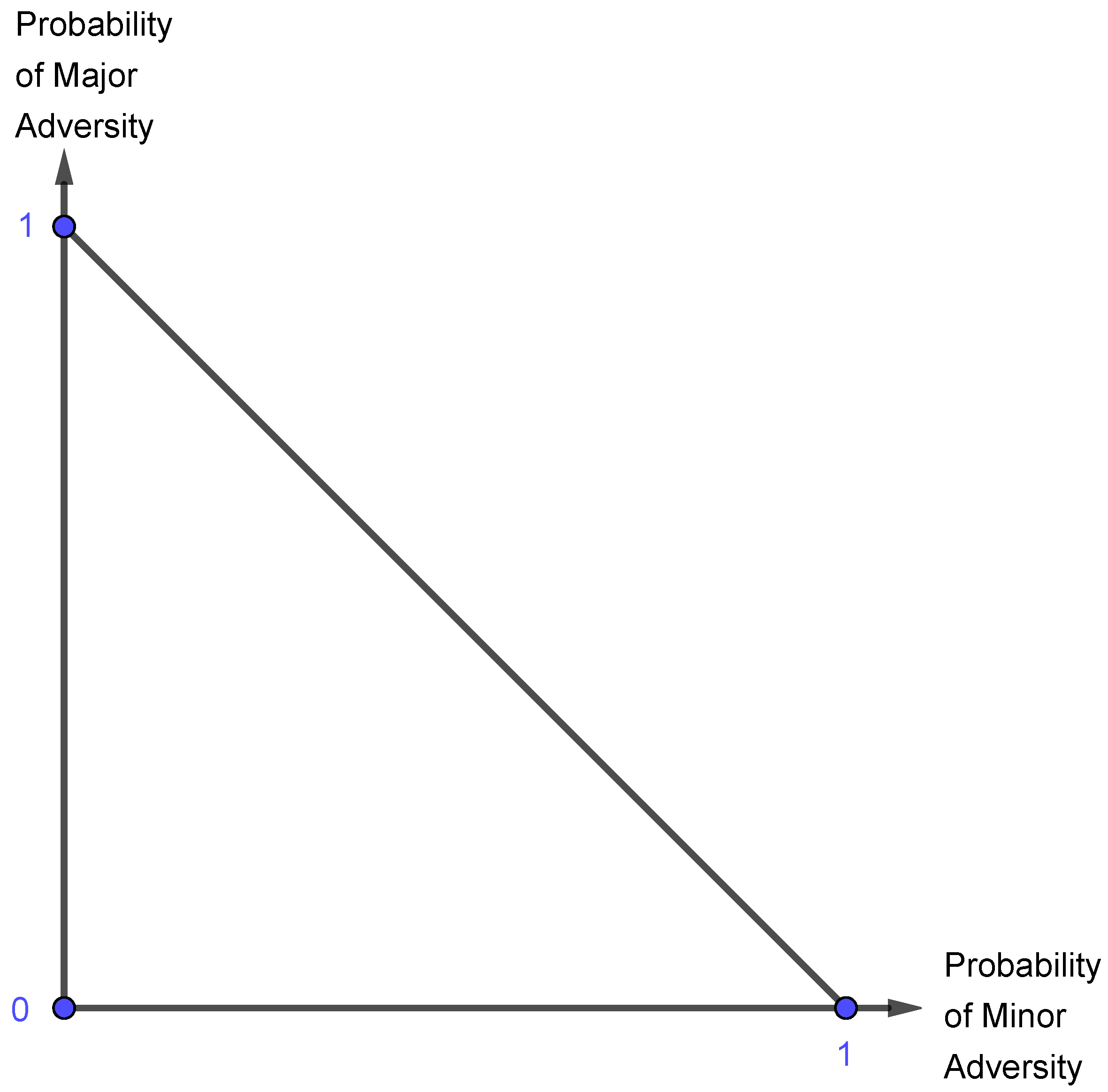
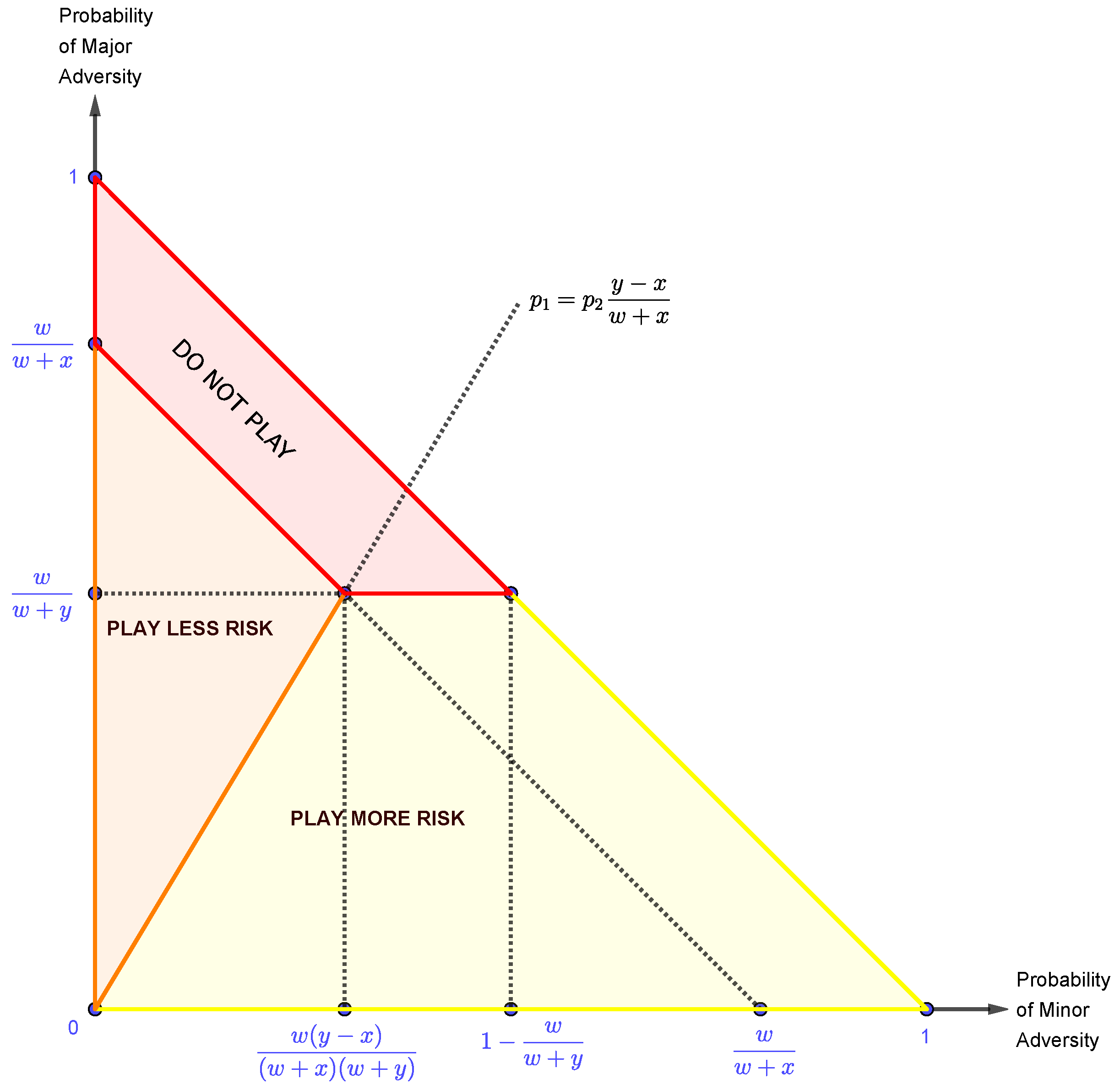
For the diagram, consider the market’s probability of playing Major Adversity on the vertical axis, and the market’s probability of playing Minor Adversity on the horizontal axis. Also, since the highest value either axis can have is

100 %

(because neither condition can prevail more than

100 %

of the time), this implies that all combinations of Major Adversity and Minor Adversity can never sum to more than

100 %

. This being the case, a diagonal line must be drawn between the

100 %

mark on both axis, which will contain all possible combinations of the market’s strategies of Major Adversity and Minor Adversity. Thus, with all of this, we obtain the following probability triangle:

Figure 9. The probability triangle showing the likelihood of loss.

We will divide this probability triangle into several regions, which will reflect when it is more advantageous to accept More or Less Risk, or even when it is advantageous not to play the game at all. Furthermore, since game theory gives us methods to determine when a player is guaranteed a certain payoff, we can solve for when it is optimal to accept either More or Less Risk.

So far, we have concentrated on the speculator’s strategies which involve taking a position in the market. However, in reality, if we know when to take a position (i.e., when to play the game), we also know when not to take a position in the market (i.e., when not to play the game). So we will develop this model in order to determine when it is advantageous to take a position, along with when it is disadvantageous to do so. Thus, conditions where it is disadvantageous to take a position will correspond to the "Do Not Play" region of the probability triangle.

Now, we can determine, with the aid of the game Table 2, the expected payoffs from playing each of the speculator’s strategies:

The Expected Payoff from playing Less Risk ( $R^{-}$ ):

$E_{S} (R^{-}) = (1 - p_{1} - p_{2}) w + p_{1} (- x) + p_{2} (- x) = w - (p_{1} + p_{2}) (w + x)$

(1)
The Expected Payoff from playing More Risk ( $R^{+}$ ):

$E_{S} (R^{+}) = (1 - p_{1} - p_{2}) w + p_{1} w + p_{2} (- y) = w - p_{2} (w + y)$

(2)

Equation (1) represents the expected payoff from playing the pure strategy Less Risk (

R^{-}

) and is written with several variables: the amount that can be won (w), the amount that can be lost due to a small stop (x), and the probability that the market will either give us minor adversity (

p_{1}

) or major adversity (

p_{2}

). Note that the speculator determines the values of w and x by his/hers risk-to-reward appetite, but the market determines the probabilities

p_{1}

and

p_{2}

If the equation 1 is greater than zero, the speculator expects a profit, but if it is less than zero, the speculator expects to lose money. Also, because the speculator is only in control of the variables x and w, we need to express the equation as strict inequality, and solve it in terms of

p_{1}

and

p_{2}

. In other words, we need to find out for which market conditions it is always advantageous to accept Less Risk by finding out when the expected payoff from playing Less Risk is greater than zero. Thus we obtain the following:

E_{S} (R^{-}) > 0 \Leftrightarrow w - (p_{1} + p_{2}) (w + x) > 0 \Leftrightarrow p_{1} + p_{2} < \frac{w}{w + x}

(3)

Note that we are considering a strict inequality because if

E_{S} (R^{-}) = 0

it is not profitable to play the Less Risk strategy, because its expected payoff is zero.

With all of this, we can incorporate equation 3 into the probability triangle yielding the following:

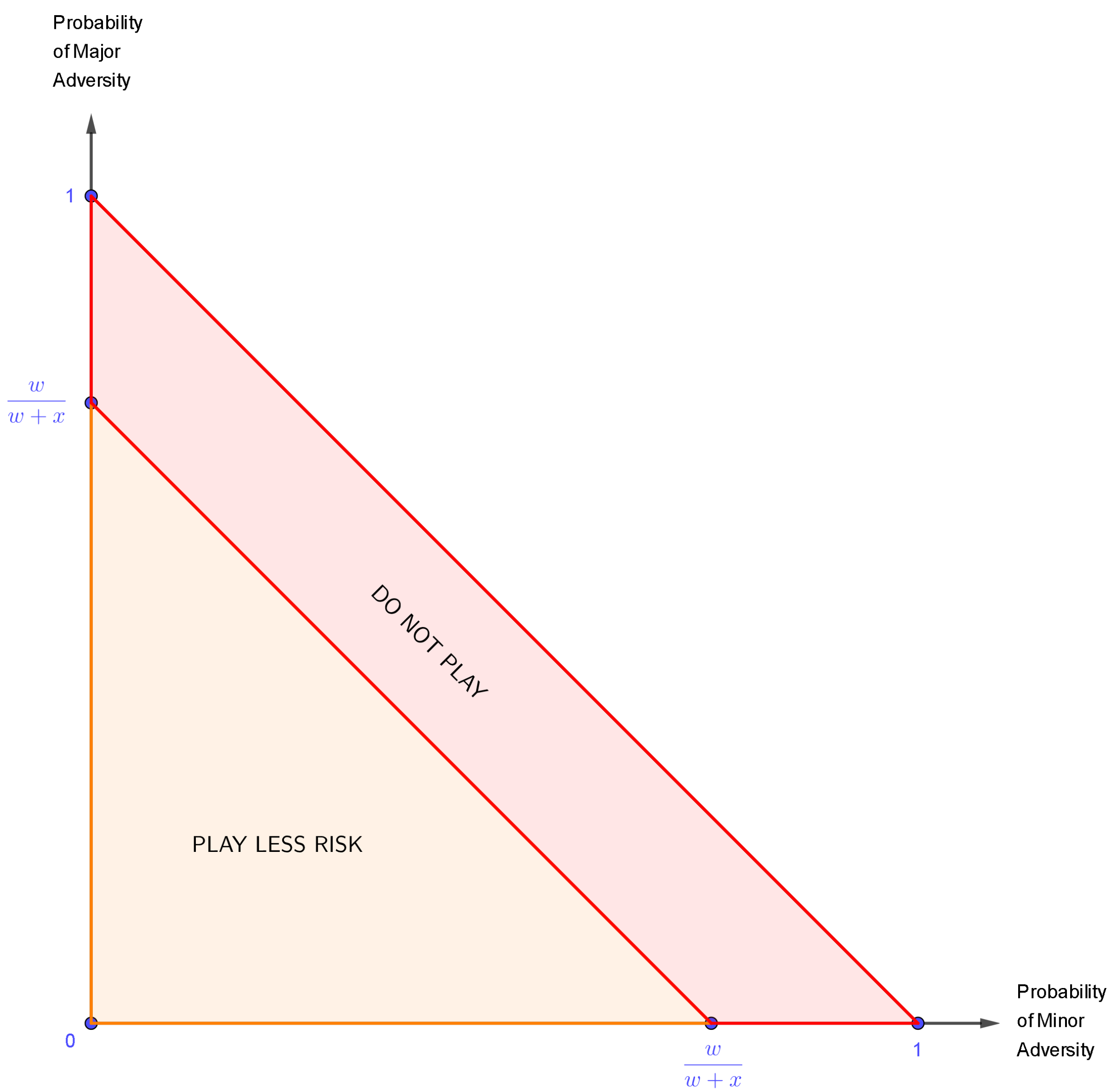
Figure 10. The probability triangle divided into two regions: "Play Less Risk" and "Do not Play".

Remark 6.

Note that, by definition of w and x:

w < w + x \Leftrightarrow \frac{w}{w + x} < 1

(4)

The "Play Less Risk" area contains the points where it is profitable to play the strategy of Less Risk, and the "Do Not Play" region contains money-losing strategies. Also, because equation 3 was developed as a strict inequality, the line diving the two regions is not included in the "Play Less Risk" area, so the points on the line (

E_{S} (R^{-}) = 0

) are included in the area of loss.

Again, the line dividing these areas is determined exclusively by the parameters set by the speculator, so this line will vary from individual to individual, always based on each individual’s risk-to-reward appetites, also the value yielded by

w / (w + x)

is not a constant that holds true for all players in the market. But, since we are developing a model in the general case, it must hold true for each and every person, no matter what their individual circumstances are.

Moving forward, we can now focus on determining when it is advantageous to accept More Risk, however it is not as straightforward as it was for Less Risk, because it is only advantageous to accept More Risk when the market is playing Minor Adversity. And, under this condition, a strategy of Less Risk will cause a small loss, but a strategy of More Risk results in a profit.

Looking back at the game Table 2:

under market conditions of Zero Adversity, both strategies yield a profit, so the speculator is indifferent between the strategies;
under market conditions of Minor Adversity, a strategy of More Risk generates a profit, and the strategy of Less Risk causes a loss, so it is advantageous to utilize the More Risk strategy;
if the market conditions correspond to Major Adversity, both the speculator’s strategies are unprofitable, but the Less Risk strategy causes a smaller loss than does the More Risk strategy, so it is less advantageous to play More Risk.

We know that, by equations 1 and 3, if the expected payoff from the Less Risk strategy is positive, then we are "guaranteed" a positive payoff when Less Risk is played. So, to find out when the strategy of More Risk yields a positive payoff when the strategy of Less Risk does not, we need to analyze equation 2 while 1 is negative.

So, we need to to find out for which market conditions it is always advantageous to accept More Risk by finding out when the Expected Payoff from playing More Risk (

R^{+}

) is greater than zero, assuming that

E_{S} (R^{-}) < 0

. Thus we obtain the following:

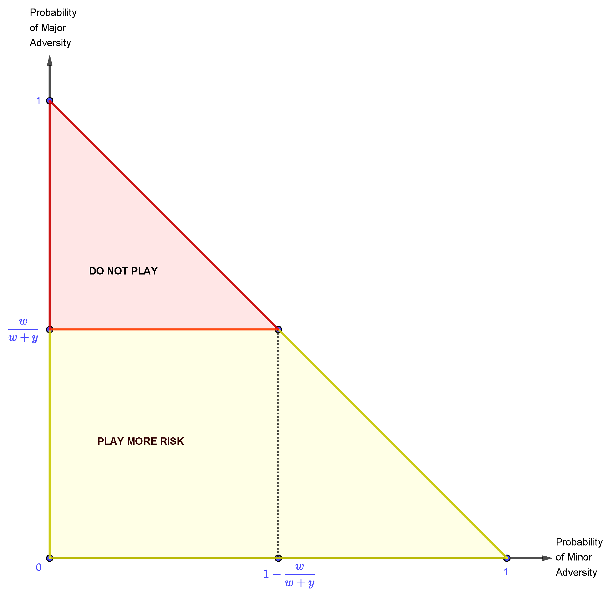
E_{S} (R^{+}) > 0 \Leftrightarrow w - p_{2} (w + y) > 0 \Leftrightarrow p_{2} < \frac{w}{w + y}

(5)

Note that we are considering a strict inequality because if

E_{S} (R^{+}) = 0

it is not profitable to play the More Risk strategy, since its expected payoff is zero. Also, observe that equation 5 is only in terms of Major Adversity (

p_{2}

) and it implies that if the probability of Major is greater than

w / (w + y)

then the trade will lose money, otherwise the trade will make money. In terms of game theory, if the probability of Major Adversity is greater than

w / (w + y)

, then we will not play the game, and if the probability of Major Adversity is less than

w / (w + y)

, then we play the pure strategy of More Risk. Additionally, if the probability of Major Adversity is equal to

w / (w + y)

, then the trade will result in a profit of zero, thus we will also not play the game.

With all of this, we can incorporate equation 5 into the probability triangle yielding the following:

Figure 11. The probability triangle divided into two regions: "Play More Risk" and "Do not Play".

Remark 7.

Regarding the previous probability triangle, note that:

by definition of w and y: $w < w + y \Leftrightarrow \frac{w}{w + y} < 1$ ;
$\{\begin{matrix} p_{2} = \frac{w}{w + y} \\ p_{1} + p_{2} = 1 \end{matrix} \Leftrightarrow \{\begin{matrix} p_{2} = \frac{w}{w + y} \\ p_{1} = 1 - \frac{w}{w + y} \end{matrix}$ .

Here, the lower region contains the conditions where it is advantageous to play the pure strategy of More Risk, and the upper region is where it is disadvantageous to play More Risk. Also, once again, the points in the separating line (

E_{S} (R^{+}) = 0

) are included in the Do Not Play area.

The same reasoning used to understand the implications of playing the pure strategy of Less Risk hold true for the strategy of More Risk, i.e., points within the "Play More Risk" area represent profitable trades and points within the "Do Not Play" area represent losses. Also, once again, the solutions must be interpreted in a probabilistic sense.

Now that we know when it is advantageous to play More Risk (assuming that the result of playing Less Risk is negative), we need determine when it is advantageous to play More Risk despite the result of playing Less Risk, because there is a region of the probability triangle where the two strategies overlap. So we still need to determine when it is advantageous to play More Risk, irrespective of the merit of playing Less Risk. Thus we need to solve the following equations:

$E_{S} (R^{+}) > 0 \Leftrightarrow w - p_{2} (w + y) > 0 \Leftrightarrow p_{2} < \frac{w}{w + y};$

(6)
$E_{S} (R^{-}) < E_{S} (R^{+}) \Leftrightarrow w - (p_{1} + p_{2}) (w + x) < w - p_{2} (w + y) \Leftrightarrow p_{1} > p_{2} \frac{y - x}{w + x} .$

(7)

Consider that equation 2 was developed as an equality, then if the probability of Minor Adversity is equal to zero (i.e.,

p_{1} = 0

), then the probability of Major Adversity has to equal to zero as well (i.e.,

p_{2} = 0

). However, in the inequality, if

p_{1}

were zero, then

p_{2}

would have to be less than zero, but this is in conflict with the variables’ definitions, because probabilities can only take values between zero and one, thus they cannot be negative. Also, the probability of Major Adversity occurring in the real world is not less than zero, because, if this were true, all the players in the market would always win. Moreover, since the formula that expresses the slope of the line (

(y - x) / (w + x)

) is always a positive number (as the variables x, y and w are all positive numbers), whenever

p_{1}

is zero, then

p_{2}

has to be zero, and vice versa. Also, the line itself represents the boundary where it is equally advantageous to play the pure risk strategies of either Less Risk or More Risk, and the area above the line defines where it is advantageous to play Less Risk.

All of these results are combined in the following probability triangle:

Remark 8.

Regarding the previous probability triangle, note that:

$\frac{w}{w + x} > 1 - \frac{w}{w + y} \Leftrightarrow \frac{w (w + y) + w (w + x)}{(w + x) (w + y)} > 1 \Leftrightarrow \frac{2 w^{2} + w x + w y}{w^{2} + w y + w x + x y} > 1 \Leftrightarrow 2 w^{2} + w x + w y > w^{2} + w y + w x + x y \Leftrightarrow w^{2} > x y$ , which is true because, by definition, $w \geq y > x$ ;
$1 - \frac{w}{w + y} > \frac{w (y - x)}{(w + x) (w + y)} \Leftrightarrow 1 > \frac{w}{w + x} \Leftrightarrow x > 0$ , which is true by definition of x;
$\{\begin{matrix} p_{1} = p_{2} \frac{y - x}{w + x} \\ p_{2} = \frac{w}{w + y} \end{matrix} \Leftrightarrow \{\begin{matrix} p_{1} = \frac{w (y - x)}{(w + x) (w + y)} \\ p_{2} = \frac{w}{w + y} \end{matrix}$ ;
$\{\begin{matrix} p_{1} = p_{2} \frac{y - x}{w + x} \\ p_{1} + p_{2} = \frac{w}{w + x} \end{matrix} \Leftrightarrow \{\begin{matrix} p_{1} = \frac{w (y - x)}{(w + x) (w + y)} \\ p_{2} = \frac{w}{w + y} \end{matrix}$ ;
$\{\begin{matrix} p_{1} + p_{2} = \frac{w}{w + x} \\ p_{2} = \frac{w}{w + y} \end{matrix} \Leftrightarrow \{\begin{matrix} p_{1} = \frac{w (y - x)}{(w + x) (w + y)} \\ p_{2} = \frac{w}{w + y} \end{matrix}$ .

In the previous probability triangle, there are three regions: the Do Not Play region, the Less Risk region, and the More Risk region. Also the dotted lines show the location of the original regions, as well some relevant intersection points. Note that all of the interior lines intersect at one point (

p_{1} = (w (y - x)) / ((w + x) (w + y)), p_{2} = w / (w + y)

), and that we included the separation line between the Less Risk and More Risk regions (i.e.,

p_{1} = p_{2} \frac{y - x}{w + x}

) in the Less Risk region, but the intersection point between all the interior lines is considered a part of the Do Not Play region.

Finally, observe that, in all of the obtained probability triangles, a "Do Not Play" region has appeared which is not related to any possible strategy (on the presented financial game) that the speculator can choose from. However, the "Do Not Play" strategy is implicit in the game Table 1 and Table 2. To see this consider the game Table 2 and that the speculator has an additional "Do Not Play" strategy. So, if the speculator chooses this strategy, then he/she will not enter the trade, and thus will not lose or win with the trade. Hence, the payoffs from this strategy are always zero independently of the market’s strategy. So, the game Table 2 becomes:

Table 3. The game table for the financial market game including the "Do Not Play" (D) strategy.

			Speculator
			$q_{1}$	$q_{2}$	$1 - q_{1} - q_{2}$
			$R^{+}$	$R^{-}$	D
Market	$p_{0}$	$0_{A}$	w	w	0
	$p_{1}$	$m_{A}$	w	$- x$	0
	$p_{2}$	$M_{A}$	$- y$	$- x$	0

However, the payoffs from adding this strategy do not change any of the calculations that we made to determine the several probability triangles, also these would only be relevant if we wanted to determine the best mixed strategy for the speculator to play (specifically, the probabilities

q_{1}

q_{2}

and

1 - q_{1} - q_{2}

would be important). But, since we only want to determine the best pure strategy that the speculator should play (i.e., one of the speculator’s probabilities will be equal to one) by taking into account the market’s probabilities (

p_{0}

p_{1}

and

p_{2}

), the "Do Not Play" strategy being explicit or not in the game table is not relevant, but this strategy is still important to the overall, because it complements the speculator’s other two strategies (Play More Risk and Play Less Risk).

So, the complete model, which incorporates all of the previous calculations and graphic representations, has the general form shown by the probability triangle in Figure 12. Also, this probability triangle represents the situation a speculator faces in a financial market, because it takes into account the speculator accepting either More Risk or Less Risk, and the market generating conditions of either Zero Adversity, Minor Adversity, or Major Adversity (always with respect to the speculator’s position). Additionally, the probability triangle has Minor Adversity and Major Adversity as its axes, yet it also shows the condition of Zero Adversity, which is the complete absence of both Major Adversity and Minor Adversity, which is represented by the origin point on the probability triangle.

Always have in mind that the model has to be interpreted in terms of "if these certain probabilities exist, then we should play a specific strategy". So the model cannot tell us what the probabilities are, it only tells us that if certain probabilities exist, then a particular strategy should be employed. Thus, if we play the financial game repeatedly, under some predetermined circumstances, the wins will outweigh the losses, and the net result of our successive plays will be profitable, this is because we need to interpret the model in the probabilistic sense rather than in an absolute sense. For instance, the model does not suggest that each and every trade that falls within the parameters of

w / (w + x)

will necessarily be profitable, only that over time the amount won will be greater than the lost.

Now that we have the complete model, we need to estimate the probabilities of the market playing the strategies of Major Adversity and Minor Adversity. Furthermore, we need to make these estimates as accurate as possible, because if they are not, the model will lose its predictive value. And we will accomplish this in the next section, with the aid of Markov Chains.

2.2. The Markov Chains Model

As we have seen in the previous section, playing the markets is an iterated game, so the next important task that we have to address is the (probabilistic) method that we will use to estimate the probabilities of the market playing Zero Adversity, Minor Adversity and Major Adversity (

p_{0}

p_{1}

and

p_{2}

respectively). However, the financial assets’ prices fluctuate from a variety of ranges (but always strictly positive). Thus we need to split the data into classes in order for us to make some kind of probabilistic analysis. For this, consider the standard deviation (

α

) of a dataset transformed with the percentage change transformation, and define the strategies’ thresholds as:

the Less Risk threshold corresponds to minus two times the standard deviation of the data ( $- 2 α$ );
the More Risk threshold corresponds to minus three times the standard deviation of the data ( $- 3 α$ );
the profit threshold corresponds to three times the standard deviation of the data ( $3 \cdot α$ ).

Since different assets from the stock market have different price ranges and levels of volatility, then by defining the thresholds in this manner, we will maintain a certain coherence across all the datasets. Also, note that the less and More Risk thresholds have to be negative, because they correspond to possible losses. Additionally, since the datasets’ unit of measure is the percentage change, the standard deviation’s unit of measure is also the percentage change.

After defining the thresholds, we can formally say what is the relationship between the market’s chosen strategies with an asset’s price. Thus, to accomplish this, we will assume that:

the asset’s price drops further than the Less Risk threshold if and only if the market chooses to play the Minor Adversity strategy;
the asset’s price drops further than the More Risk threshold if and only if the market chooses to play the Major Adversity strategy;
the asset’s price increases further than the profit threshold if and only if the market chooses to play the Zero Adversity strategy.

Now, consider that we observed the asset’s percentage price change for N successive and mutually independent financial market games, and that we want to determine the mentioned probabilities for the next (

N + 1

) game. Also, the percentage price change of game i is denoted by

X_{i}

i = 1, \dots, N + 1

. Additionally, assume that if the thresholds of Major Adversity or Zero Adversity are reached in a game, suppose that it was on game

k \in {1, \dots, N}

, then the speculator will not play on the following games,

k + 1, \dots, N

, otherwise the speculator will continue to play. We need to assume this because, if the speculator loses or wins on a game, then we will not continue playing, due to the trade being closed, and if the price does not reach one of the thresholds, the speculator will not win nor lose the game, so he/she needs to keep playing, because the trade is still open.

Remark 9.

Note that if the market chooses to play Minor Adversity, the speculator only has to stop playing if he/she played the Less Risk strategy.

With all of this, we can start estimating the desired probabilities for the

{(N + 1)}^{t h}

game, knowing that the probability of the market playing a certain strategy at game

N + 1

is related to the probabilities of the market’s choices on the N previous games, i.e., we want to determine

p_{0} = P (X_{N + 1} \geq 3 \cdot α | X_{1}, \dots, X_{N}),

p_{2} = P (X_{N + 1} \leq - 3 \cdot α | X_{1}, \dots, X_{N}),

p_{1} = 1 - p_{0} - p_{2} .

Remark 10.

Note that we will not directly estimate

p_{1}

, because it is simpler to estimate

p_{0}

and

p_{2}

, due to the way we defined these probabilities. Also, we can do this because

p_{0} + p_{1} + p_{2} = 1

. So, moving forward, we will not reference the estimator of

p_{1}

unless we see fit to do so.

Firstly, suppose that we only consider one game to determine our probabilities, i.e., we will start by considering

N = 1

, so we have the following:

$p_{2} = P (X_{2} \leq - 3 \cdot α | X_{1}) = P (X_{1} \leq - 3 \cdot α);$

(8)
$p_{0} = P (X_{2} \geq 3 \cdot α | X_{1}) = P (X_{1} \geq 3 \cdot α) .$

(9)

We can interpret equation 10 for the probability of the market playing Major Adversity as follows: if the percentage price change reaches the More Risk threshold in game 1, then the speculator stops playing. So, the probability of the price change reaching the More Risk threshold is obtained by simply calculating the probability of the percentage change reaching the More Risk threshold in the previous game, i.e.,

P (X_{1} \leq - 3 \cdot α)

Similarly, the probability of the market playing the Zero Adversity strategy is obtained by calculating the probability of the percentage change reaching the profit objective threshold in the previous game, i.e.,

P (X_{1} \geq 3 \cdot α)

However, since we have access to more historical data of the asset’s price, we can determine these probabilities more accurately by taking into account more games. Now, consider that we will use the results of two past games to determine our probabilities, i.e., we will consider

N = 2

, thus we obtain:

\begin{matrix} \begin{matrix} p_{2} & = P (X_{3} \leq - 3 \cdot α | X_{2}, X_{1}) = & (10) \\ \begin{matrix} = P (X_{1} \leq - 3 \cdot α) + P (- 3 \cdot α < X_{1} \leq 3 \cdot α \land X_{2} \leq - 3 \cdot α); \end{matrix} & (11) \end{matrix} \end{matrix}

\begin{matrix} p_{0} = P (X_{3} \geq 3 \cdot α | X_{2}, X_{1}) = P (X_{1} \geq 3 \cdot α) + P (X_{1} < 3 \cdot α \land X_{2} \geq 3 \cdot α) . \end{matrix}

(12)

Thus we can can interpret the new equation 10 for the probability of the market playing Major Adversity as follows: the speculator stops playing, if the percentage price change reaches the More Risk threshold in game 1 or if the threshold is only reached in game 2 (implying that, in game 1, no threshold was reached). So, the probability of the price change reaching the More Risk threshold is obtained by adding the probability of the percentage change reaching the More Risk threshold in game 1 to the probability of the percentage change reaching the More Risk threshold in game 2 without reaching it in game 1. And, a similar interpretation can be given to equation 11.

Finally, we can obtain even more accurate probabilities if we consider the results of all the played games (i.e., by considering all the historical price data). Thus, considering the results of N games, the equations for the desired probabilities are:

\begin{matrix} \begin{matrix} p_{2} & = P (X_{N + 1} \leq - 3 \cdot α | X_{N}, \dots, X_{1}) = \\ = P (X_{1} \leq - 3 \cdot α) + P (- 3 \cdot α < X_{1} < 3 \cdot α \land X_{2} \leq - 3 \cdot α) + \\ + P (- 3 \cdot α < X_{1} < 3 \cdot α \land - 3 \cdot α < X_{2} < 3 \cdot α \land X_{3} \leq - 3 \cdot α) + \dots + \\ + P (- 3 \cdot α < X_{1} < 3 \cdot α \land - 3 \cdot α < X_{2} < 3 \cdot α \land - 3 \cdot α < X_{3} < 3 \cdot α \land \\ \land \dots \land - 3 \cdot X_{N} \leq - 3 \cdot α) . \end{matrix} \end{matrix}

(13)

\begin{matrix} \begin{matrix} p_{0} & = P (X_{N + 1} \geq 3 \cdot α | X_{N}, \dots, X_{1}) = P (X_{1} \geq 3 \cdot α) + P (X_{1} < 3 \cdot α \land X_{2} \geq 3 \cdot α) + \\ + P (X_{1} < 3 \cdot α \land X_{2} < 3 \cdot α \land X_{3} \geq 3 \cdot α) + \dots + \\ + P (X_{1} < 3 \cdot α \land X_{2} < 3 \cdot α \land X_{3} < 3 \cdot α \land \dots \land X_{N} \geq 3 \cdot α); \end{matrix} \end{matrix}

(14)

The intuition behind the obtained equations 14 and 13 is similar to the one that we used to obtain the equations 8 and 9. Also, because the N games are mutually independent, from basic probability theory we have that the equations 14 and 13 are equivalent to:

\begin{matrix} \begin{matrix} p_{2} & = P (X_{N + 1} \leq - 3 \cdot α | X_{N}, \dots, X_{1}) = \\ = P (X_{1} \leq - 3 \cdot α) + P (- 3 \cdot α < X_{1} < 3 \cdot α) P (X_{2} \leq - 3 \cdot α) + \\ + P (- 3 \cdot α < X_{1} < 3 \cdot α) P (- 3 \cdot α < X_{2} < 3 \cdot α) P (X_{3} \leq - 3 \cdot α) + \dots + \\ + P (- 3 \cdot α < X_{1} < 3 \cdot α) P (- 3 \cdot α < X_{2} < 3 \cdot α) P (- 3 \cdot α < X_{3} < 3 \cdot α) \dots \\ \dots P (- 3 \cdot X_{N} \leq - 3 \cdot α) \end{matrix} \end{matrix}

(15)

\begin{matrix} \begin{matrix} p_{0} & = P (X_{N + 1} \geq 3 \cdot α | X_{N}, \dots, X_{1}) = P (X_{1} \geq 3 \cdot α) + P (X_{1} < 3 \cdot α) P (X_{2} \geq 3 \cdot α) + \\ + P (X_{1} < 3 \cdot α) P (X_{2} < 3 \cdot α) P (X_{3} \geq 3 \cdot α) + \dots + \\ + P (X_{1} < 3 \cdot α) P (X_{2} < 3 \cdot α) P (X_{3} < 3 \cdot α) \dots P (X_{N} \geq 3 \cdot α); \end{matrix} \end{matrix}

(16)

From these equations we can see that, for example, to estimate

p_{0}

(and

p_{2}

), we would have to estimate

(N (N + 1)) / 2

probabilities, which would be computationally inefficient and the error from the final estimate would increase due to the large number of individual estimates. So, to overcome these problems we will use Markov chains to estimate the probabilities

p_{0}

p_{1}

and

p_{2}

Thus, using the same assumptions and notations as before:

the asset’s percentage price change for N successive financial market games is known;
the percentage price change of game i is denoted by $X_{i}$ , $i = 1, \dots, N + 1$ ;
we want to determine the mentioned probabilities the ${N + 1}^{t h}$ game;
if any of thresholds is reached in a game, suppose that it was on game $k \in {1, \dots, N}$ , then the speculator will not play on the following games, $k + 1, \dots, N$ , otherwise the speculator will continue to play.

Now, because we will use Markov Chains, we need to assume that the probabilities associated with each game are related through the Markov property (for further details see [31]):

Definition 1

(Markov Property). A stochastic process

{x_{t}, t = 0, 1, 2, \dots}

with a discrete and finite (or countable) state space S is said to be a Markov chain if for all states

i_{0}, i_{1}, \dots, i_{t - 1}, i, j

and (steps)

t \geq 0

P (x_{t + 1} = j | x_{0} = i_{0}, \dots, x_{t - 1} = i_{t - 1}, x_{t} = i) = P (x_{t + 1} = j | x_{t} = i) = p_{i j}^{t, t + 1} .

So, we obtain the following estimators for

p_{0}

and

p_{2}

$p_{0} = P (X_{N + 1} \geq 3 \cdot α | X_{N}, \dots, X_{1}) = P (X_{N + 1} \geq 3 \cdot α | X_{N});$

(17)
$p_{2} = P (X_{N + 1} \leq - 3 \cdot α | X_{N}, \dots, X_{1}) = P (X_{N + 1} \leq - 3 \cdot α | X_{N}) .$

(18)

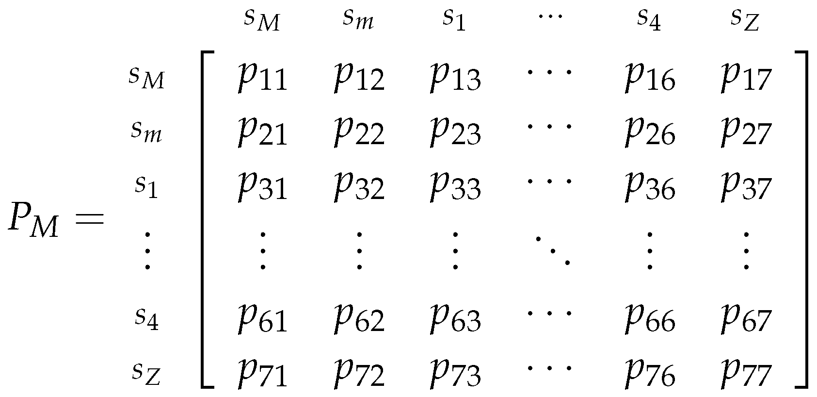
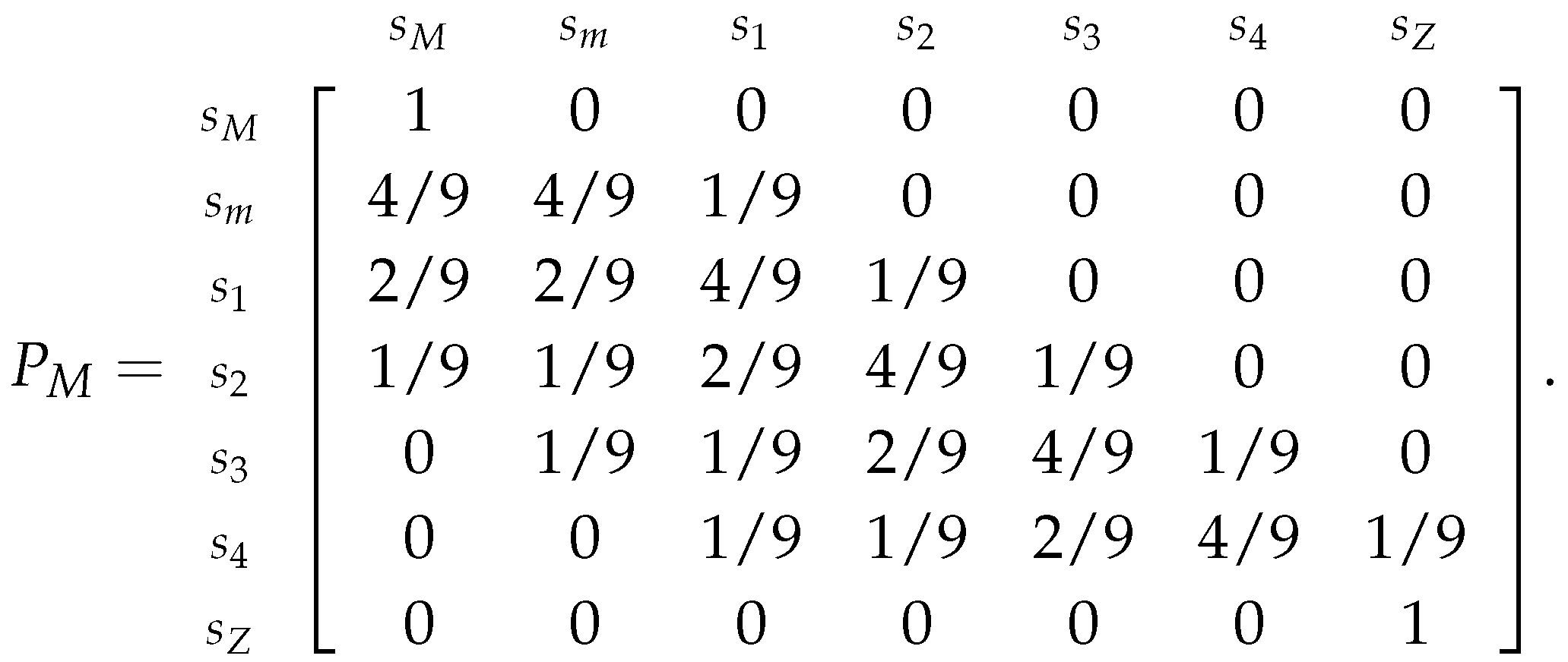
In order for us to be able to use the percentage price change (of a given asset) at game i (i.e., to use

X_{i}

) as the underlying stochastic process of the Markov chain, we need to split the data into classes (or states). Also, by defining the Markov chain we will obtain its probability matrix, which will allow us to estimate

p_{0}

and

p_{2}

Before moving further, we need to note that, for instance, if the price is (at a certain time) on a lower price class (relative to the initial price), then it will have a higher probability of transitioning to a higher price class, due to the nature of the data that we are utilizing, and a similar argument can be made if the price is on a higher class (as we have seen in Chapter 1). However, this is represented by the Markov property, because the probability of the Markov chain being in a certain state at time t only depends on which state the chain was at time

t - 1

, so this probability may change according to which states the chain encounters itself in time

t - 1

. And this fact will also affect on how we will define the chain’s classes.

To define the classes we can utilize the standard deviation (which we previously denoted by

α

) of the dataset, and since we defined (and used) the strategies’ thresholds, we will split the data "around" these thresholds values, also the classes’ ranges and distance between them will be

α

Additionally, due to the mentioned volatility and wide range of the assets’ prices, they may reach one of the thresholds in the first game (or iteration), or they may not reach them at all. So, for these reasons we will define some intermediate classes between the the classes associated with the thresholds (or market strategies). Thus, with all of this, we obtain that the classes (or states) are:

the Major Adversity class is

$s_{M} = {X_{t} : X_{t} \leq - 2.5 \cdot α};$

(19)
the Minor Adversity class is

$s_{m} = {X_{t} : - 2.5 \cdot α < X_{t} \leq - 1.5 \cdot α};$

(20)
the intermediate classes between Minor Adversity and the Zero Adversity classes are:
- $s_{1} = {X_{t} : - 1.5 \cdot α < X_{t} \leq - 0.5 \cdot α};$
  
  (21)
- $s_{2} = {X_{t} : - 0.5 \cdot α < X_{t} \leq 0.5 \cdot α};$
  
  (22)
- $s_{3} = {X_{t} : 0.5 \cdot α < X_{t} \leq 1.5 \cdot α};$
  
  (23)
- $s_{4} = {X_{t} : 1.5 \cdot α < X_{t} \leq 2.5 \cdot α} .$
  
  (24)
the Zero Adversity (or Profit) class is

$s_{Z} = {X_{t} : X_{t} > 2.5 \cdot α} .$

(25)

Remark 11.

Note that, instead of using the previously defined threshold to limit the classes, we chose to define the classes around these thresholds, in order to include them. However, if all the classes maintain a certain coherence according to the thresholds and have the same range (excluding the

s_{M}

and

s_{Z}

classes), then we will obtain similar results after applying our models.

As an example, consider the dataset

{45.00, 44.49, 43.44, 40.17, 41.05, 41.53, 41.36, 40.68, 40.46, 38.42}

(26)

to be the prices of some financial asset for ten consecutive days, then its percentage change transformed dataset (rounded to two decimal cases) is:

{- 1.13, - 2.36, - 7.53, 2.19, 1.17, - 0.41, - 1.64, - 0.54, - 5.04},

(27)

which was obtained by applying the percentage changes transformation. So, the standard deviation of this transformed dataset is

3.00

(which also is a percentage), i.e.,

α = 3.00

. Hence the classes, for this example, are:

$s_{M} = {X_{t} : X_{t} \leq - 2.5 \cdot α} = {X_{t} : X_{t} \leq - 7.5}$ ;
$s_{m} = {X_{t} : - 2.5 \cdot α < X_{t} \leq - 1.5 \cdot α} = {X_{t} : - 7.5 < X_{t} \leq - 4.5}$ ;
$s_{1} = {X_{t} : - 1.5 \cdot α < X_{t} \leq - 0.5 \cdot α} = {X_{t} : - 4.5 < X_{t} \leq - 1.5}$ ;
$s_{2} = {X_{t} : - 0.5 \cdot α < X_{t} \leq 0.5 \cdot α} = {X_{t} : - 1.5 < X_{t} \leq 1.5}$ ;
$s_{3} = {X_{t} : 0.5 \cdot α < X_{t} \leq 1.5 \cdot α} = {X_{t} : 1.5 < X_{t} \leq 4.5}$ ;
$s_{4} = {X_{t} : 1.5 \cdot α < X_{t} \leq 2.5 \cdot α} = {X_{t} : 4.5 < X_{t} \leq 7.5}$ ;
$s_{Z} = {X_{t} : X_{t} > 2.5 \cdot α} = {X_{t} : X_{t} > 7.5}$ .

2.2.1. Defining the Markov Chains

Before formally defining the necessary Markov Chains, we need to make some observations about the described classes. According to our assumptions, if the market chooses to play Major Adversity or Zero Adversity, the speculator will have to stop playing (which will result in a major a loss or in a profit, respectively) independently of the speculator’s chosen strategy, but if the market chooses to play Minor Adversity, the speculator only has to stop playing if he/she chose the Less Risk strategy.

Also, with the aid of game table 2 (from the previous section (2.1)), we can see that the results of the market playing the Major Adversity strategy are only noticeable if the speculator chooses to play the More Risk strategy, because if the speculator chooses the Less Risk strategy he/she will stop playing the game immediately after the Less Risk threshold is reached, thus he/she will not know if the price further increased or decreased.

Thus, assuming that the speculator chose the More Risk strategy, we can determine the probability of the market playing the Major Adversity strategy. Also, if we assume that the speculator chose to play the Less Risk strategy, then we can determine the probability of the market playing the Zero Adversity strategy, this is because, in this case, the speculator only has a profit if the market chooses this strategy.

So, for these reasons we will define two Markov Chains, one where we consider that the speculator chose the Less Risk strategy and another where he/she chose to play the More Risk strategy. However, we will always use the same assumptions, strategies’ thresholds and data for both the Markov Chains, so that we can utilize the probability matrices from each to estimate the probabilities

p_{0}

p_{1}

and

p_{2}

. Also, we will assume that

s_{2} = {X_{t} : 0.5 \cdot α < X_{t} \leq 0.5 \cdot α}

is the initial state for both the Markov chains, because when the speculator enters for trade of a certain asset, then the asset’s initial percentage price change will be

0 %

which is an element of the

s_{2}

class.

Regarding the Markov Chain where we assume that the speculator chose to play the More Risk strategy, we have the following observations about its states (or classes):

The classes $s_{M}, s_{m}, s_{1}, \dots, s_{4}, s_{Z}$ will retain the same definitions as before
To represent the fact that the speculator only stops playing if the price enters the Major Adversity class ( $s_{M}$ ) or the Zero Adversity class ( $s_{Z}$ ) in the Markov Chain, we simply must define these classes as absorbing states, i.e., if the price enters one of these classes, then it will never exit them (for more details see [30,31] and/or [34]).
Since the speculator does not stop playing if the price is in one of the remaining classes, the price may go to any class (including staying in the same class). And, to represent this in terms of Markov Chains, we simply define these classes as transient (for more details see [30,31,34] and/or[35]). Also, these states ( $s_{m}, s_{1}, \dots, s_{4}$ ) communicate between themselves, thus they form a communicating class in the Markov Chain.

In the terms of Markov Chains, for this Markov Chain, we are considering the stochastic process

{X_{t}, t = 1, 2, \dots, N}

, where

X_{t}

is the percentage price change at game t, with a discrete and finite state space

S = {s_{M}, s_{m}, s_{1}, \dots, s_{4}, s_{Z}}

, where for all states

S_{0}, S_{1}, \dots, S_{t - 1}, S_{i}, S_{j} \in S

and steps (or games)

t \in {1, \dots, N}

P (X_{t + 1} = S_{j} | X_{1} = S_{0}, \dots, X_{t - 1} = S_{t - 1}, X_{t} = S_{i}) = P (X_{t + 1} = S_{j} | X_{t} = S_{i}) = : p_{i j}^{t, t + 1} .

Here, the steps of the Markov Chain represent each successive game from 1 up until N, and

S_{i}

represents a state from the state space

S = {s_{M}, s_{m}, s_{Z}, s_{1}, \dots, s_{4}}

, which is composed by the classes that we previously defined, thus they have the mentioned properties. Also, the

7 \times 7

transition matrix

P_{M}

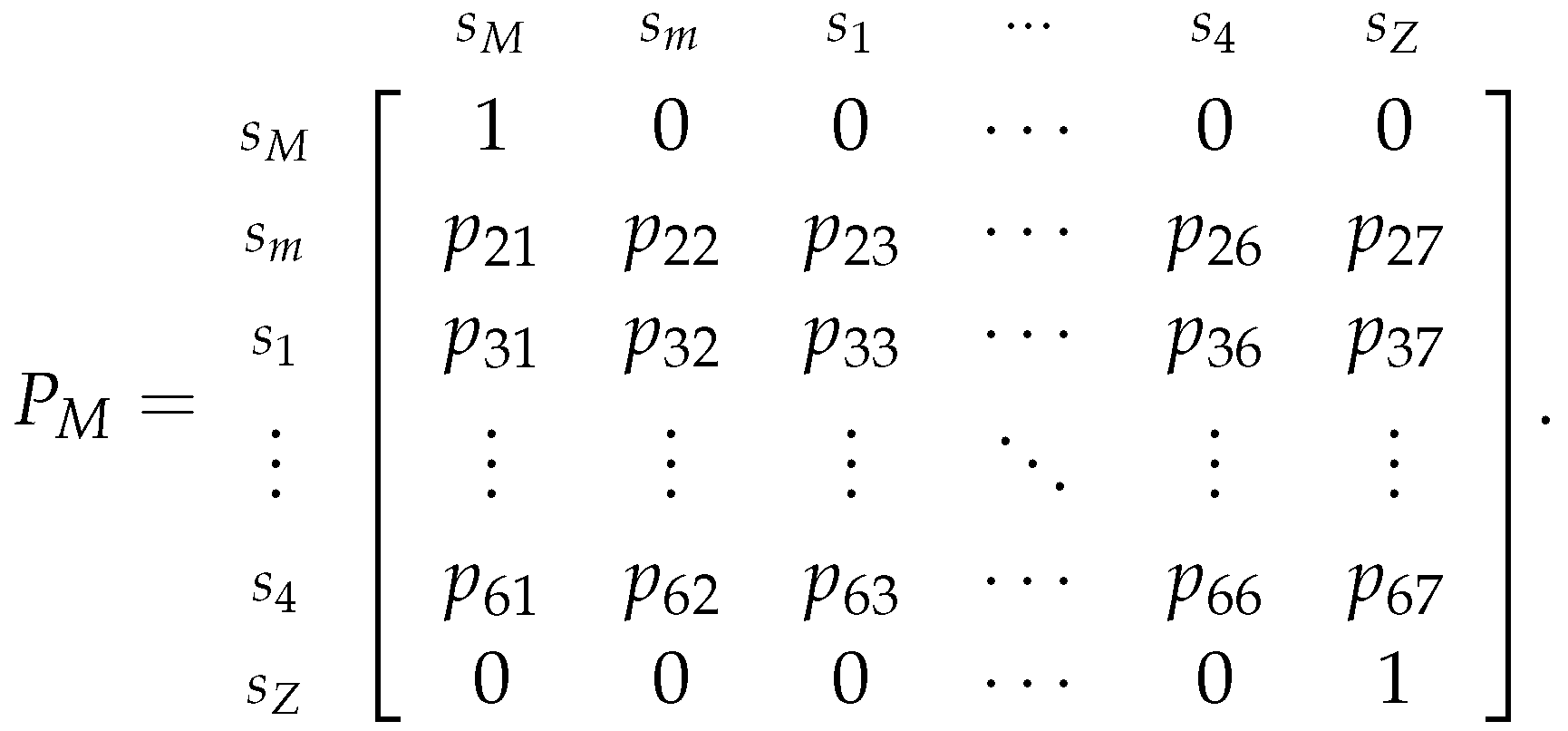
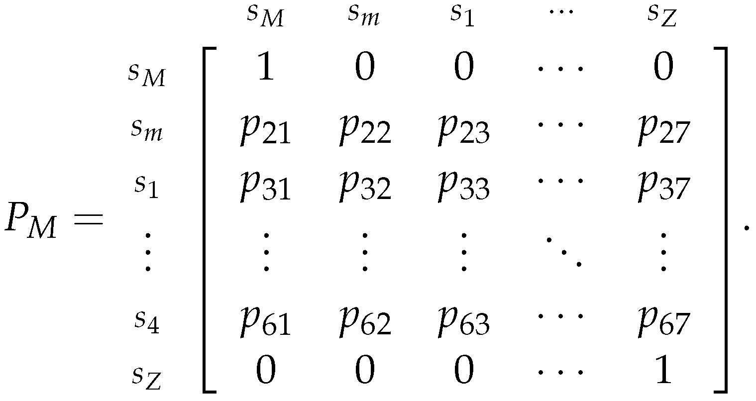
associated with this chain will be defined as:

(28)

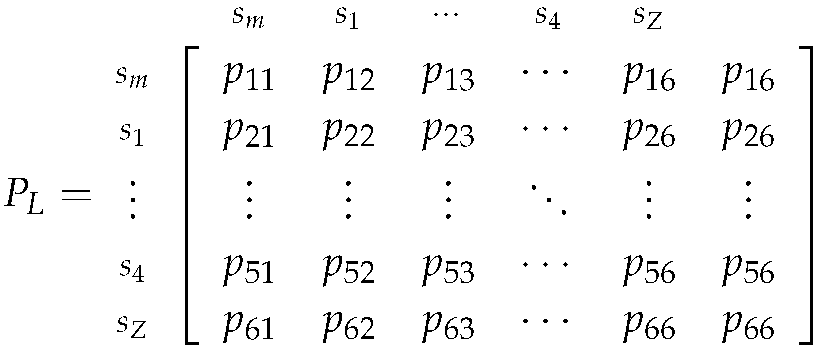
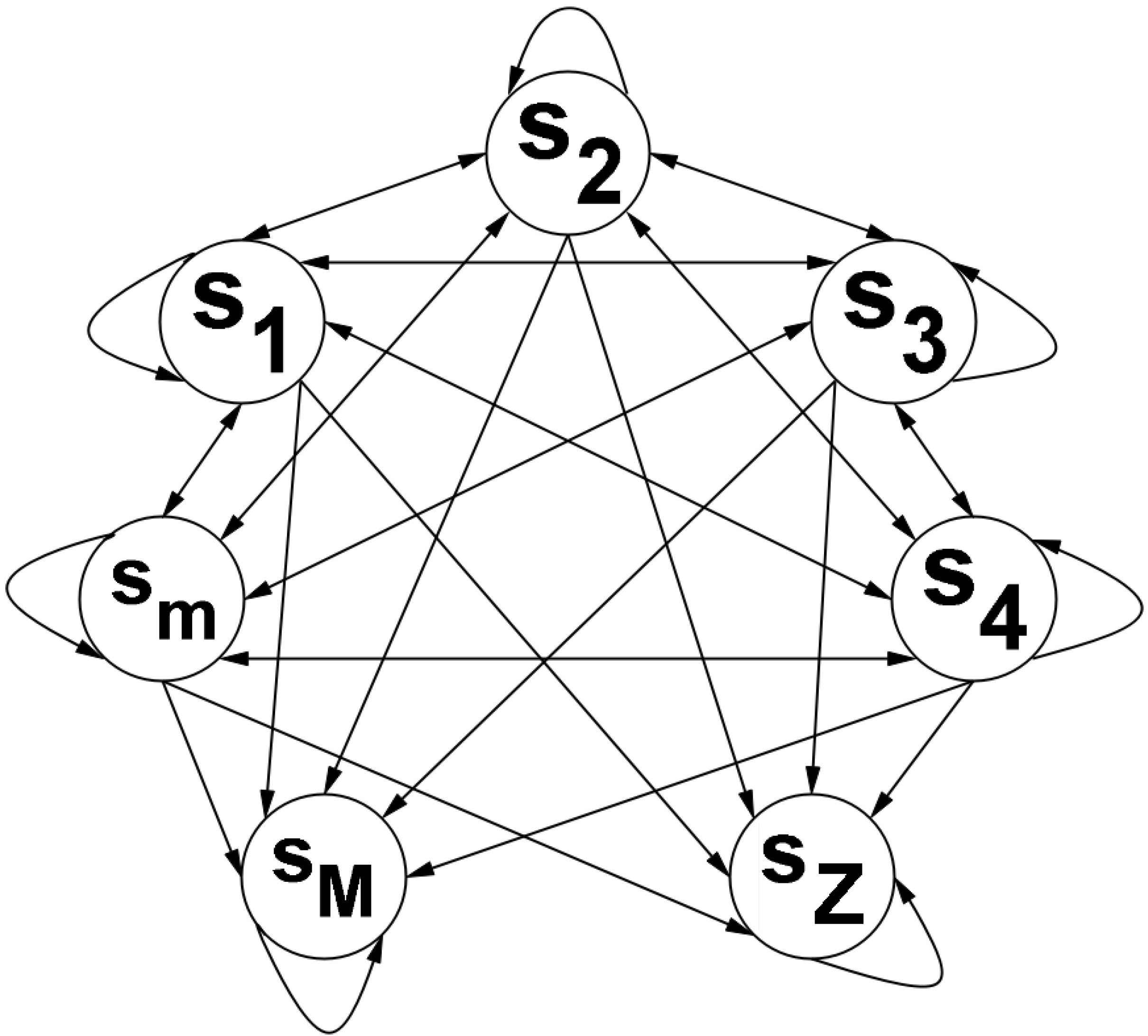
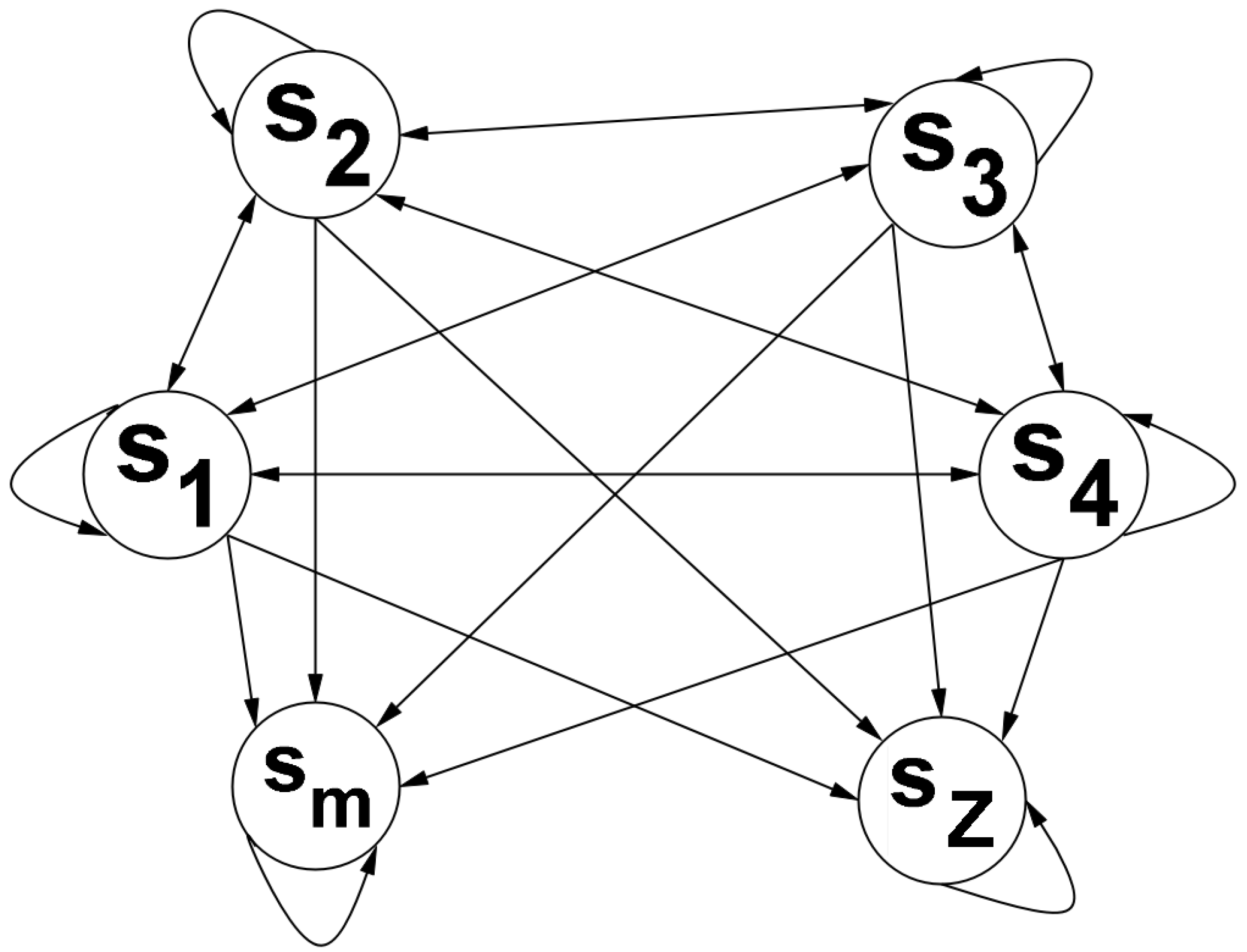
To visualize this Markov Chain we can use the following diagram:

Note that we could have simplified the previous diagram by joining the states

s_{m}, s_{1}, \dots, s_{4}

in the same communicating class. However, it is useful for us to present the Markov chain in this manner, because it allow us to take more conclusions on how the chain develops as we move forward in time.

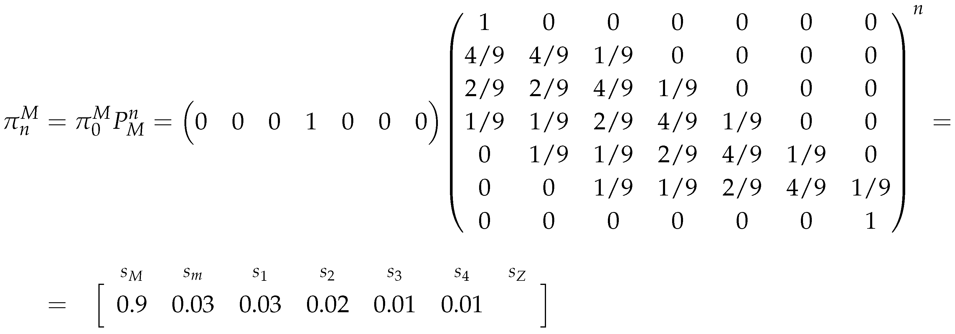
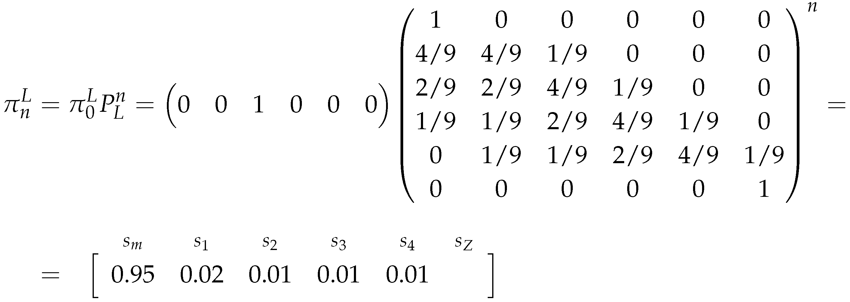
So, assuming that the initial state is

s_{2}

(i.e., assuming that

π = {(0, 0, 0, 1, 0, 0, 0)}^{T}

) and that the transition matrix

P_{M}

related to the Markov chain is well defined, the probability of the market playing the Major Adversity strategy (

p_{2}

) at time (or game) t is given by the first element of

π P_{M}^{t}

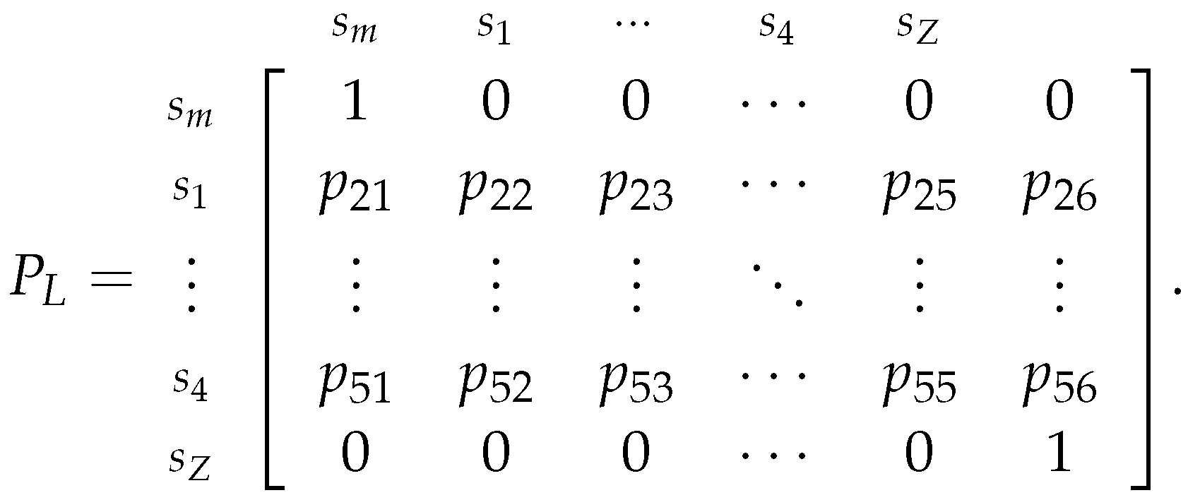
Now, regarding the Markov Chain where we assume that the speculator chose to play the Less Risk strategy, we can make similar observations as before, but with some modifications:

The Major Adversity class is not necessary for this Markov chain, because the speculator will stop playing if the price reaches the Minor Adversity class. So the $s_{M}$ class will be "included" in the $s_{m}$ class, thus $s_{m}$ is altered to $s_{m} = {X_{t} : X_{t} \leq - 1.5 \cdot α}$ (considering Example 26, this class becomes $s_{m} = {X_{t} : X_{t} \leq - 4.5}$ ).
The classes $s_{Z}, s_{1}, \dots, s_{4}$ are defined as before.
To represent the fact that the speculator stops playing if the price enters the Minor Adversity class ( $s_{m}$ ) or the Zero Adversity class ( $s_{Z}$ ) in the Markov Chain, we simply must define these classes as absorbing states, i.e., if the price enters one of these classes, then it will never exit them (for more details see [30,31] and/or [34]).
Since the speculator does not stop playing if the price is in one of the remaining classes, the price may go to any class (including staying in the same class). And, to represent this in terms of Markov Chains, we simply define these classes as transient (for more details see [30,31,34] and/or[35]).

As before, in the terms of Markov Chains, we are considering the same stochastic process

{X_{t}, t = 1, 2, \dots, N}

, where

X_{t}

is the percentage price change at game t, with a discrete and finite state space

S = {s_{m}, s_{Z}, s_{1}, \dots, s_{4}}

, where for all states

S_{0}, S_{1}, \dots, S_{t - 1}, S_{i}, S_{j} \in S

and steps (or games)

t \in {1, \dots, N}

P (X_{t + 1} = S_{j} | X_{1} = S_{0}, \dots, X_{t - 1} = S_{t - 1}, X_{t} = S_{i}) = P (X_{t + 1} = S_{j} | X_{t} = S_{i}) = : p_{i j}^{t, t + 1} .

Here, the steps of the Markov Chain represent each successive game from 1 up until N, and

S_{i}

represents a state from the state space

S = {s_{m}, s_{Z}, s_{1}, \dots, s_{4}}

, which is composed by the classes that we previously defined, thus they have the mentioned properties. Also, the

6 \times 6

transition matrix

P_{L}

associated with this chain will be defined as:

(29)

To visualize this Markov Chain we can use the following diagram:

Regarding this diagram, note that is its similar to the previous one (13), however, in this one, the state

s_{M}

is included in the state

s_{m}

. Additionally, we could have simplified the diagram by joining the states

s_{1}, \dots, s_{4}

in the same communicating class. But again, it is useful for us to present the Markov chain in this manner, for the same reasons as before.

So, assuming that the initial state is

s_{2}

(i.e., assuming that

π = {(0, 0, 1, 0, 0, 0)}^{T}

) and that the transition matrix

P_{L}

related to the Markov chain is well defined, the probability of the market playing the Zero Adversity strategy (

p_{0}

) at time/game t is given by the last element of

π P_{L}^{t}

With all of this, we have the necessary methods to estimate the probabilities of the market playing Zero Adversity, Minor Adversity and Major Adversity, thus we also have a method on how to choose the best strategy for a certain dataset. However, the estimation method for the market’s probabilities is not complete, because we still have to estimate the transition probability matrix for each of the defined Markov chains. So, this is what we will focus on until the end of this section. But, before moving further, note that:

we will always use the same (percentage change transformed) dataset for all of the estimations;
since the $s_{Z}$ state is absorbing in both of the chains, then we do not need to estimate its transition probabilities, i.e., the last row of both the transition matrices (28 and 29) is of the form $(0, \dots, 0, 1)$ ;
the state $s_{M}$ in the Markov chain related to the More Risk strategy, like the $s_{Z}$ state, is absorbing, thus the first row of the transition matrix 28 is of the form $(1, 0, \dots, 0)$ ;
the state $s_{m}$ in the Markov chain related to the Less Risk strategy, like the $s_{Z}$ state, is absorbing, thus the first row of the transition matrix 29 is of the form $(1, 0, \dots, 0)$ .

2.2.2. Estimation of the Transition Probabilities

To estimate the transition probabilities for each of the Markov chains, lets start by considering the one where we assume that the speculator chose to play the More Risk strategy, represented by the following transition matrix (similar to the previously presented matrix 28):

(30)

Now, lets consider that we are departing from state

s_{2} = {X_{t} : 0.5 \cdot α < X_{t} \leq 0.5 \cdot α}

(the assumed initial state of the chain), so to estimate the transition probabilities

{p_{41}, p_{42}, p_{43}, \dots, p_{47}}

, we will just determine the relative frequency of each of the sates using the dataset, and we will use these frequencies on the corresponding row of the transition matrix.

Utilizing the Example 26, the relative frequencies for the transformed dataset for these classes are:

Table 4. Relative frequencies table considering that the starting state is

s_{2}

Table 4. Relative frequencies table considering that the starting state is

s_{2}

$s_{M}$	$s_{m}$	$s_{1}$	$s_{2}$	$s_{3}$	$s_{4}$	$s_{Z}$
$\frac{1}{9}$	$\frac{1}{9}$	$\frac{2}{9}$	$\frac{4}{9}$	$\frac{1}{9}$	$09$	$09$

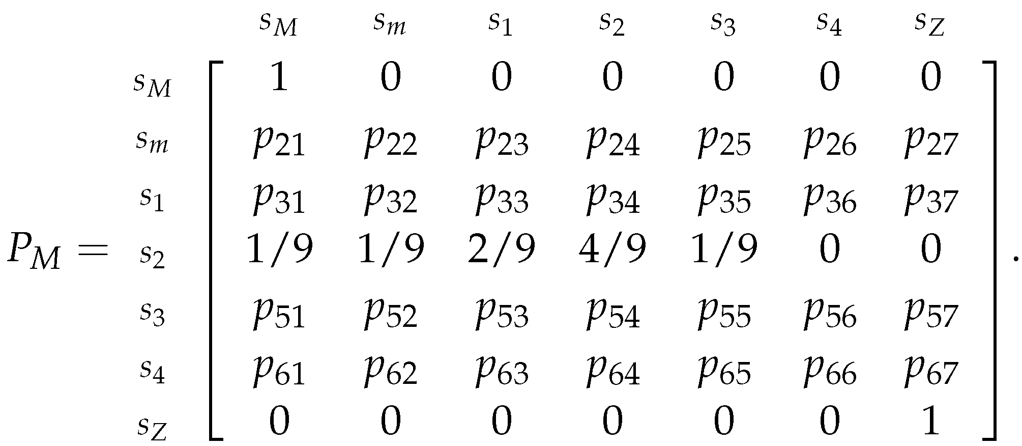
And, replacing in the transition matrix (related to Example 26’s Markov chain), we obtain:

(31)

As it was previously observed, the probabilities of transitioning from state

s_{2}

(to any other state) are not the same as if we considered that we started from a different state. Thus, in order to take this into account and to still use the relative frequency "method" to estimate the transition probabilities, we need to slightly alter the classes on which we will determine the relative frequencies.

For example, consider the classes obtained from Example 26, if the price increased

3 %

(of its initial price) at the first iteration of the chain, i.e., the price went from

100 %

103 %

of its (initial) value (which translates in a

((103 - 100) / 100) * 100 = 3 %

percentage change in price), then the chain moved from state

s_{2}

to the state

s_{3}

. However, if the price is now at the state

s_{3}

and it further increased

3 %

(comparing to the initial price), the chain will not move from the

s_{3}

state to the

s_{4}

state, because , in this case, the price went from

103 %

106 %

of its (initial) value, so the percentage change in price is

((106 - 103) / 103) * 100 \approx 2.91 %

, which is not a member of the

s_{4}

state, thus the chain will remain in the

s_{3}

state. So, the transition from the

s_{3}

state to all of the other states is not the same (in terms of percentage change) as the transition from

s_{2}

to all of the other states. And, a similar argument can be made if we considered that we started from any state different from

s_{2}

With this in mind, if we want to use the relative frequencies of the dataset to estimate the transitions from any state to any other, then we need to "re-calculate" the classes in order for the estimation to be coherent with what we assumed and defined. So, to accomplish this, we need to consider the percentage change of price regarding the previous iteration of the chain, and not the percentage change regarding the initial price.

Again, for example, to estimate the transition from the

s_{3}

state to the

s_{4}

state, we need to assume that the initial state is the

s_{3}

state and that we want to transition to the

s_{4}

state, i.e., we need to assume the percentage price change (relative to the

s_{2}

) is at

103 %

and that we want to know what is the percentage price change if the percentage price change transitioned to

106 %

(relative to the

s_{2}

), which would be

((106 - 103) / 103) * 100 \approx 2.91 %

. Also, because we are dealing with classes, this obtained percentage change between classes will be used as the "new"

α

to determine the limits (and ranges) of the classes, this is because

s_{3}

and

s_{4}

are consecutive classes in terms of their range of values (as

s_{2}

and

s_{3}

were in the base classes). Thus, in this case, the

s_{4}

state (or class) becomes

s_{4} = {X_{t} : 1.46 < X_{t} \leq 4.37}

. So, we need to use these "re-calculated" classes to obtain the relative frequencies table, which will be the estimation for the transition probabilities if we consider that we started from state

s_{3}

To generally define the classes which we will use in the relative frequencies table, we need to consider the direct correspondence

f : {s_{m}, s_{1}, s_{2}, s_{3}, s_{4}} \to {2, 1, 0, - 1, - 2}

defined as:

\begin{matrix} f (s_{m}) = 2 \\ f (s_{1}) = 1 \\ f (s_{2}) = 0 \\ f (s_{3}) = - 1 \\ f (s_{4}) = - 2 \end{matrix}

So, the "altered" classes (or states) obtained considering that we started from state

s \in {s_{m}, s_{1}, s_{2}, s_{3}, s_{4}}

are:

$s_{M} = {X_{t} : X_{t} \leq (- 2.5 + f (s)) \cdot α};$

(32)
$s_{m} = {X_{t} : (- 2.5 + f (s)) \cdot α < X_{t} \leq (- 1.5 + f (s)) \cdot α};$

(33)
$s_{1} = {X_{t} : (- 1.5 + f (s)) \cdot α < X_{t} \leq (- 0.5 + f (s)) \cdot α};$

(34)
$s_{2} = {X_{t} : (- 0.5 + f (s)) \cdot α < X_{t} \leq (0.5 + f (s)) \cdot α};$

(35)
$s_{3} = {X_{t} : (0.5 + f (s)) \cdot α < X_{t} \leq (1.5 + f (s)) \cdot α};$

(36)
$s_{4} = {X_{t} : (1.5 + f (s)) \cdot α < X_{t} \leq (2.5 + f (s)) \cdot α};$

(37)
$s_{Z} = {X_{t} : X_{t} > (2.5 + f (s)) \cdot α} .$

(38)

Note that, the value of

α

used in the equations of the new classes, also needs to be re-calculated, which we will see how to do so after determining the "re-calculated" classes for the Example 26 considering that we started from the

s_{3}

state and with

α = 2.91

, which are:

$s_{M} = {X_{t} : X_{t} \leq - 10.185}$ ;
$s_{m} = {X_{t} : - 10.185 < X_{t} \leq - 7.275}$ ;
$s_{1} = {X_{t} : - 7.275 < X_{t} \leq - 4.365}$ ;
$s_{2} = {X_{t} : - 4.365 < X_{t} \leq - 1.455}$ ;
$s_{3} = {X_{t} : - 1.455 < X_{t} \leq 1.455}$ ;
$s_{4} = {X_{t} : 1.455 < X_{t} \leq 4.365}$ ;
$s_{Z} = {X_{t} : X_{t} > 4.365}$ .

Utilizing the dataset from Example 26, we have the following relative frequencies table for these classes:

Table 5. Relative frequencies table considering that the starting state is

s_{3}

Table 5. Relative frequencies table considering that the starting state is

s_{3}

$s_{M}$	$s_{m}$	$s_{1}$	$s_{2}$	$s_{3}$	$s_{4}$	$s_{Z}$
$09$	$\frac{1}{9}$	$\frac{1}{9}$	$\frac{2}{9}$	$\frac{4}{9}$	$\frac{1}{9}$	$09$

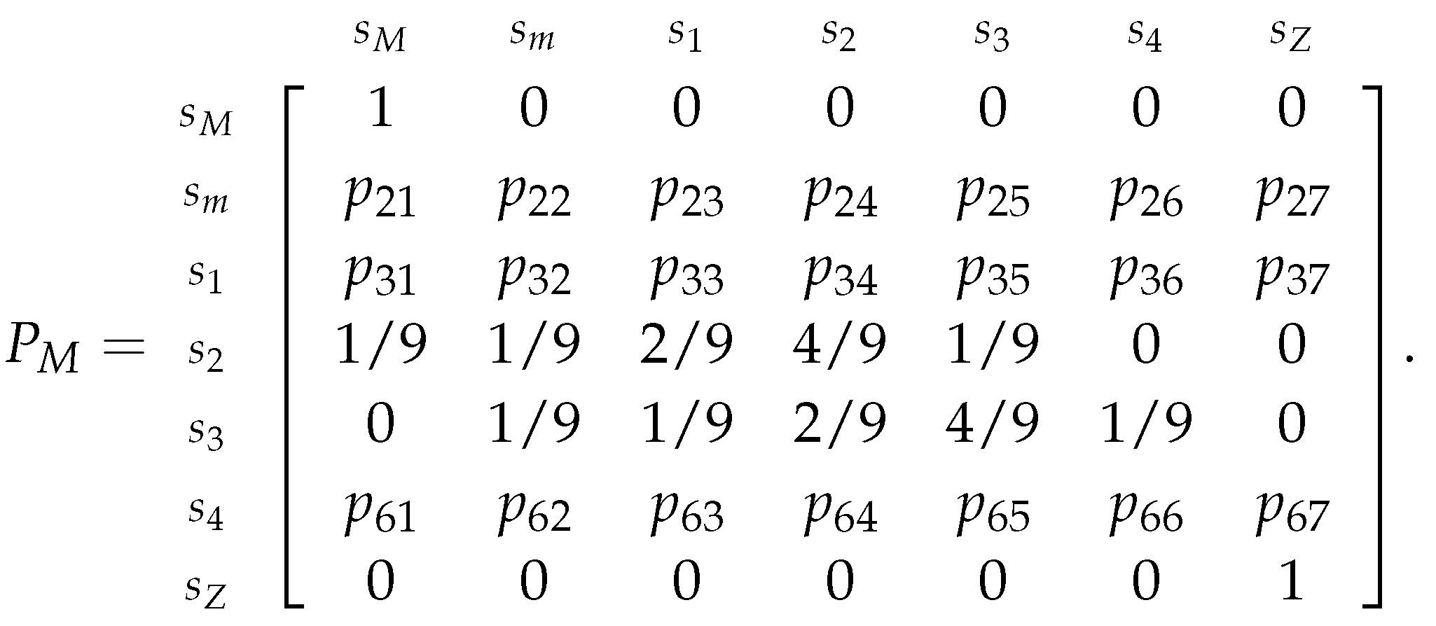
Replacing in the transition matrix 31 (related to Example 26’s Markov chain), we obtain:

(39)

Now, for the general case, consider that we want to determine the relative frequencies assuming that we are departing from the

s_{i} \in {s_{m}, s_{1}, \dots, s_{4}}

state, then we need to determine the range of each class, i.e., we need to determine the

α

that we will use in the previously presented formulas 32-38. For this, we need to consider

s_{i}

’s consecutive class, which is the class that contains the values immediately before the lower limit of

s_{i}

or after the upper limit of

s_{i}

, and we will denote it as

s_{j}

. Also, it is not relevant which of the two that we choose. For instance, if

s_{i} = s_{m}

, then its consecutive classes are

s_{M}

and

s_{1}

, so

s_{j}

can be either

s_{M}

s_{m}

; likewise, the (only) consecutive class of

s_{i} = s_{M}

s_{j} = s_{m}

. Thus, after obtaining the consecutive class, consider

m_{i}

and

m_{j}

to be the midpoints of

s_{i}

and

s_{j}

, respectively. But, if

s_{j}

s_{M}

s_{Z}

m_{j}

will be the

m_{i} + (i n f (s_{i}) - s u p (s_{i}))

m_{i} + (s u p (s_{i}) - i n f (s_{i}))

, respectively.

So, the

α

value is obtained by:

α = |\frac{m_{j} - m_{i}}{m_{i} + 100} 100| .

(40)

Remark 12.

Note that we did not include

s_{M}

and

s_{Z}

into the set of possible states that

s_{i}

can be, this is because the probabilities of departing from these states are fixed, as we saw when we built the transition matrix 30. Also, in the calculation of the α, we need to consider the absolute value, in case

s_{j}

is related to lower limit of

s_{i}

Afterwards, we simply have to determine the classes by replacing the obtained

α

in all of the equations 32-38, which we will use to calculate the relative frequencies table of the (same transformed) dataset. Finally, we just replace the obtained relative frequencies in the row of the transition matrix related to the

s_{i}

state (or class).

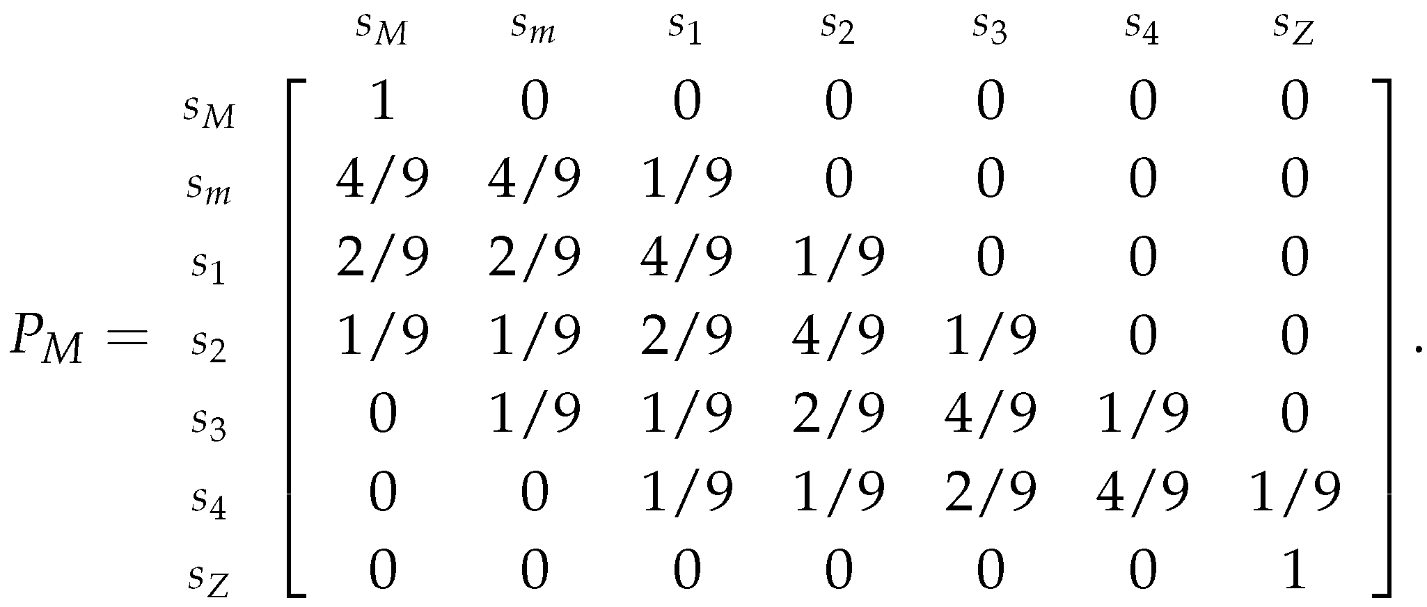
Applying all of this to example 26, we obtain the following transition matrix:

(41)

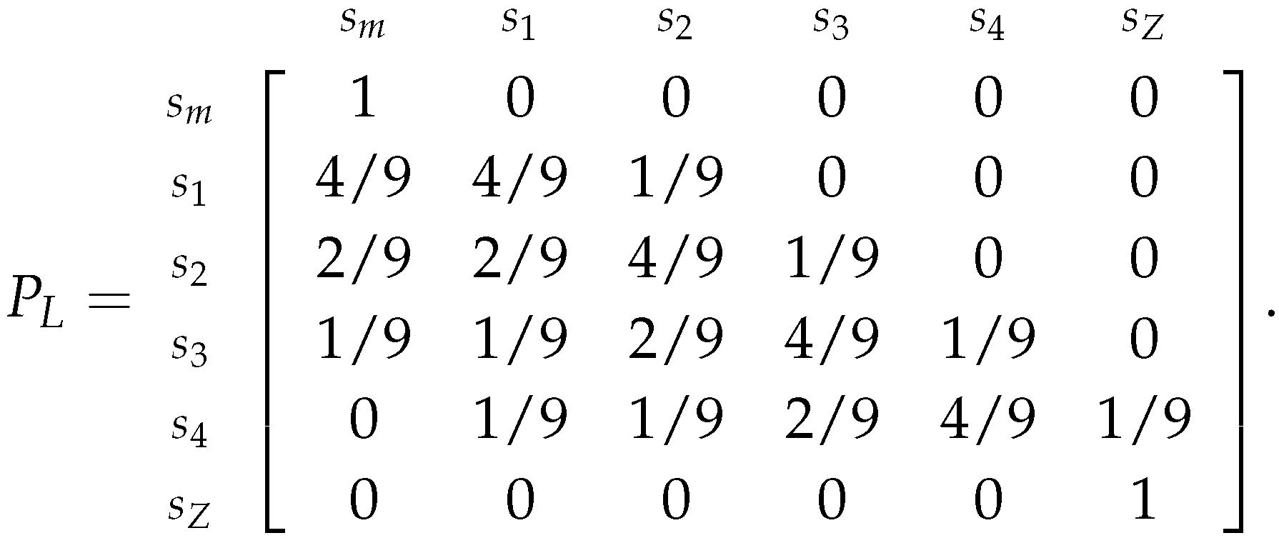
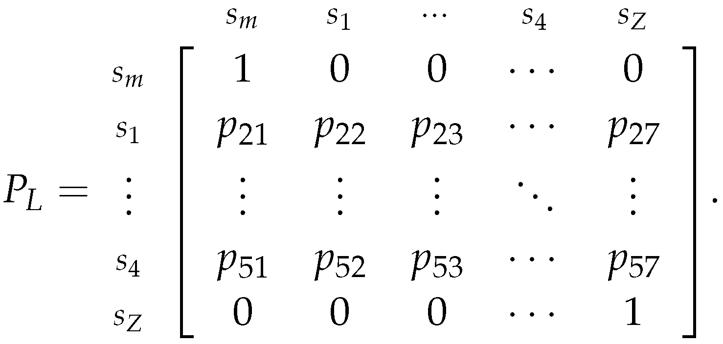
All the presented estimators and examples are related to the Markov Chain where we assume that the speculator chose to play the More Risk strategy. So, to estimate the transition probabilities for the Markov Chain where we assume that the speculator chose to play the Less Risk strategy, which is represented by the following transition matrix (similar to the previously presented matrix 29):

(42)

And, like in the

P_{M}

case, we will determine the relative frequency tables considering that the chain started from each of the sates

s_{1}, \dots, s_{4}

. So, again assume that we are departing from the

s_{i} \in {s_{1}, \dots, s_{4}}

state, then we need to determine the range of each class, i.e., we need to determine the

α

that we will use in formulas similar to the previously presented ones (32-38). So, as before, consider a consecutive class to

s_{i}

, denoted as

s_{j}

. For instance, if

s_{i} = s_{1}

, then its consecutive classes are

s_{m}

and

s_{2}

, so

s_{j}

can be either

s_{m}

s_{2}

; likewise, the (only) consecutive class of

s_{i} = s_{m}

s_{j} = s_{1}

. After obtaining the consecutive class, consider

m_{i}

and

m_{j}

to be the midpoints of

s_{i}

and

s_{j}

, respectively. But, if

s_{j}

s_{m}

s_{Z}

m_{j}

will be the

m_{i} + (i n f (s_{i}) - s u p (s_{i}))

m_{i} + (s u p (s_{i}) - i n f (s_{i}))

, respectively.

So, the

α

value is obtained by:

α = |\frac{m_{j} - m_{i}}{m_{i} + 100} 100| .

(43)

Remark 13.

Note that the equation to obtain α in the

P_{L}

case is the same as the previous equation 40. Also, we did not include

s_{m}

and

s_{Z}

into the set of possible states that

s_{i}

can be, this is because the probabilities of departing from these states are fixed, as we observed when we built the transition matrix 29.

As in the

P_{M}

case, the transition probabilities are not the same as if we considered that the chain started from different states. Thus, in order to take this into account and to still use the relative frequency "method" to estimate the transition probabilities we need to slightly alter the classes on which we will determine the relative frequencies. So, again consider the direct correspondence

f : {s_{1}, \dots, s_{4}} \to {2, 1, 0, - 1, - 2}

defined as:

\begin{matrix} f (s_{1}) = 1 \\ f (s_{2}) = 0 \\ f (s_{3}) = - 1 \\ f (s_{4}) = - 2 \end{matrix}

So, the "altered" classes (or states) for the

P_{L}

matrix considering that we started from a state

s \in {s_{1}, \dots, s_{4}}

are:

$s_{m} = {X_{t} : X_{t} \leq (- 1.5 + f (s)) \cdot α};$

(44)
$s_{1} = {X_{t} : (- 1.5 + f (s)) \cdot α < X_{t} \leq (- 0.5 + f (s)) \cdot α};$

(45)
$s_{2} = {X_{t} : (- 0.5 + f (s)) \cdot α < X_{t} \leq (0.5 + f (s)) \cdot α};$

(46)
$s_{3} = {X_{t} : (0.5 + f (s)) \cdot α < X_{t} \leq (1.5 + f (s)) \cdot α};$

(47)
$s_{4} = {X_{t} : (1.5 + f (s)) \cdot α < X_{t} \leq (2.5 + f (s)) \cdot α} .$

(48)
$s_{Z} = {X_{t} : X_{t} > (2.5 + f (s)) \cdot α} .$

(49)

Now, we will estimate the

P_{L}

matrix for the same dataset

{45.00, 44.49, 43.44, 40.17, 41.05, 41.53, 41.36, 40.68, 40.46, 38.42}

from Example 26, which resulted into the transformed dataset

{- 1.13, - 2.36, - 7.53, 2.19, 1.17, - 0.41, - 1.64, - 0.54, - 5.04} .

Considering that we started from the

s_{3}

state (with the consecutive state

s_{4}

), i.e., considering that:

α = |\frac{m_{j} - m_{i}}{m_{i} + 100} 100| = |\frac{6 - 3}{3 + 100} 100| \approx 2.91 .

We obtain the classes

$s_{m} = {X_{t} : X_{t} \leq - 7.275}$ ;
$s_{1} = {X_{t} : - 7.275 < X_{t} \leq - 4.365}$ ;
$s_{2} = {X_{t} : - 4.365 < X_{t} \leq - 1.455}$ ;
$s_{3} = {X_{t} : - 1.455 < X_{t} \leq 1.455}$ ;
$s_{4} = {X_{t} : 1.455 < X_{t} \leq 4.365}$ ;
$s_{Z} = {X_{t} : X_{t} > 4.365}$ .

And, by replacing the relative frequencies,

P_{L}

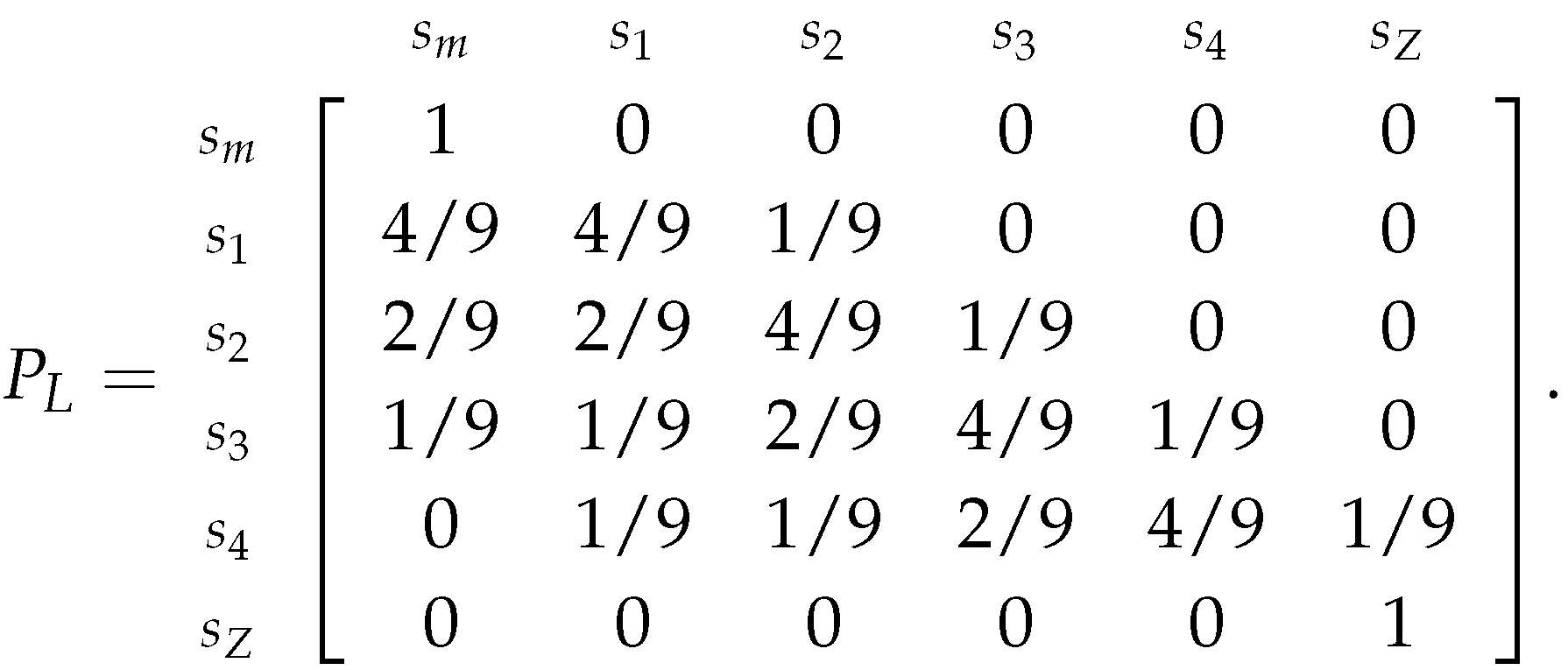
is:

(50)

2.2.3. Estimating the Market’s Probabilities

Now, we have everything that we need to estimate the probabilities of the market playing Zero Adversity (

p_{0}

), Minor Adversity (

p_{1}

) and Major Adversity (

p_{2}

). And, to accomplish this, we will use two Markov chains to estimate

p_{2}

and

p_{0}

, as it was previously explained.

To estimate

p_{2}

we will make the use of the Markov Chain where we assumed that the speculator chose to play the More Risk strategy, which is represented by the transition matrix 30:

(51)

Also, as before, we will assume that the initial state of the chain is

s_{2}

, i.e., the probability distribution of

X_{0}

(the first percentage price change of the chain) is given by the

π_{0}^{M} = {(0, 0, 0, 1, 0, 0, 0)}^{T}

Since we want to predict what will happen to an asset’s price after we buy it, that is, we want to know if we will have a profit or a loss (according to the financial game that we established) after we enter a trade, then it is sensible to consider what will happen immediately after we buy the asset and/or what is the asset’s price tending to. So, to this end, we will consider two separate estimators and analyze the obtained results. Thus,

p_{2}

will be estimated by:

the probability of the chain reaching the $s_{M}$ state after one iteration;
the long-run probability of the chain being at state $s_{M}$ .

Regarding the first estimator, we will just compute the probability of the chain being at state

s_{M}

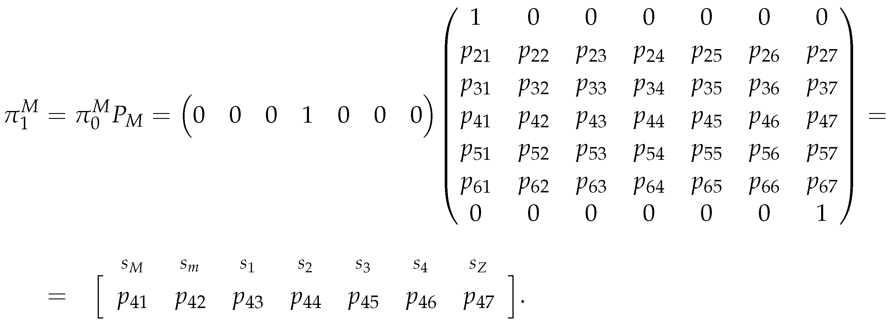
after one iteration of the chain, so we will compute:

Where, after the matrix multiplication, we obtained a

1 \times 7

vector

π_{1}^{M}

, which is the probability distribution of the chain after one iteration. Here, note that

π_{1}^{M}

is simply the transition probabilities starting from the

s_{2}

state, which makes sense considering that the initial state is

s_{2}

and we only want to know the probability distribution after one iteration of the chain. Thus, the first entry of

π_{1}^{M}

is the probability of the chain being in state

s_{M}

after one iteration and our estimator for

p_{2}

is:

p_{2} \approx p_{41} .

As we can see, this estimator is fairly simple, both in theoretical and in practical terms. So, to try to understand how the percentage price will evolve, we will also consider a estimator related to the long term distribution of the chain. However, we need to note that this probability distribution may not exist, because our chain is not irreducible. So, we cannot use Theorem II.C.3 from [31] to guarantee that such distribution exists. Also, if such distribution is to exist, we know (from [30,34]) that the chain will tend to its absorbing states, thus, in our case, the long run probability distribution would be a

1 \times 7

vector

π

where one of the absorbing states (

s_{M}

s_{Z}

) has a probability of one. But, we do not know when this will happen or which state will have probability one. Hence, to overcome these issues, we will compute the probability distribution of the chain after

n < \infty

iterations:

\begin{matrix} π_{n}^{M} & = π_{0}^{M} P_{M}^{n} = (\begin{matrix} 0 & 0 & 0 & 1 & 0 & 0 & 0 \end{matrix}) {(\begin{matrix} 1 & 0 & 0 & 0 & 0 & 0 & 0 \\ p_{21} & p_{22} & p_{23} & p_{24} & p_{25} & p_{26} & p_{27} \\ p_{31} & p_{32} & p_{33} & p_{34} & p_{35} & p_{36} & p_{37} \\ p_{41} & p_{42} & p_{43} & p_{44} & p_{45} & p_{46} & p_{47} \\ p_{51} & p_{52} & p_{53} & p_{54} & p_{55} & p_{56} & p_{57} \\ p_{61} & p_{62} & p_{63} & p_{64} & p_{65} & p_{66} & p_{67} \\ 0 & 0 & 0 & 0 & 0 & 0 & 1 \end{matrix})}^{n} = \end{matrix}

(52)

(53)

Thus, after the matrix multiplication, we obtain a

1 \times 7

vector

π_{n}^{M}

, and its first entry is the probability of the chain being in state

s_{M}

after n iterations, so our estimator for

p_{2}

is:

p_{2} \approx π_{n 1} .

Observe that we cannot apply the Theorem II.C.3 from [31] to determine the long-run probability distribution

π

of the chain, because it is not irreducible. So, we do need to compute the n matrix multiplications.

Now, similarly to the estimator of

p_{2}

, we will estimate

p_{0}

using the Markov Chain where we assumed that the speculator chose to play the Less Risk strategy, which is represented by the transition matrix 42:

(54)

As before, we will assume that the initial state of the chain is

s_{2}

, i.e., we will assume that

π_{0}^{L} = {(0, 0, 1, 0, 0, 0)}^{T}

. So, for the same reasons as before,

p_{0}

will be estimated by:

the probability of the chain reaching the $s_{Z}$ state after one iteration;
the long-run probability of the chain being at state $s_{Z}$ .

Regarding the first estimator, we will just compute the probability of the chain being at state

s_{Z}

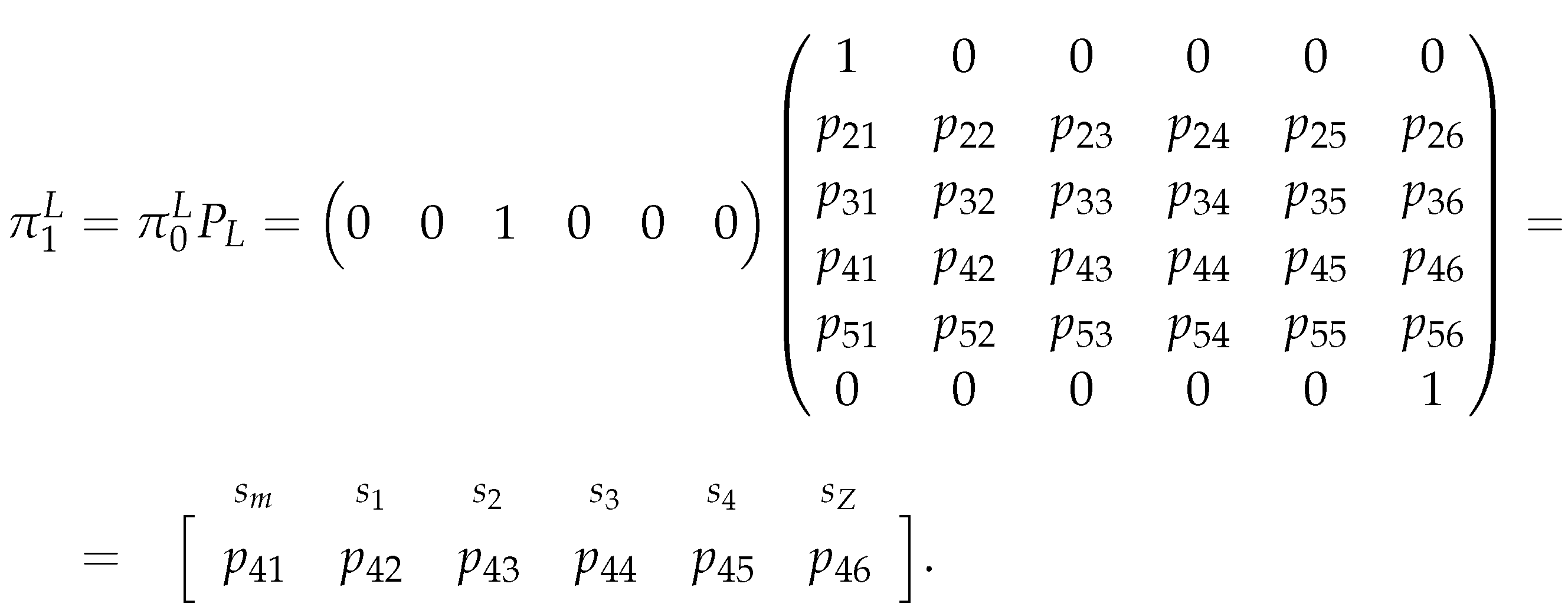
after one iteration of the chain, i.e. we will compute:

Where, after the matrix multiplication, we obtain a

1 \times 6

vector

π_{1}^{L}

. And, again, note that

π_{1}

is simply the transition probabilities starting from the

s_{2}

state. Also, the last entry of

π_{1}^{L}

is the probability of the chain being in state

s_{Z}

after one iteration, so our estimator for

p_{0}

is:

p_{0} \approx p_{46} .

As before, this estimator is fairly simple, and because this chain is also not irreducible, we will compute the probability distribution (

π_{n}^{L}

) of the chain again after

n < \infty

iterations:

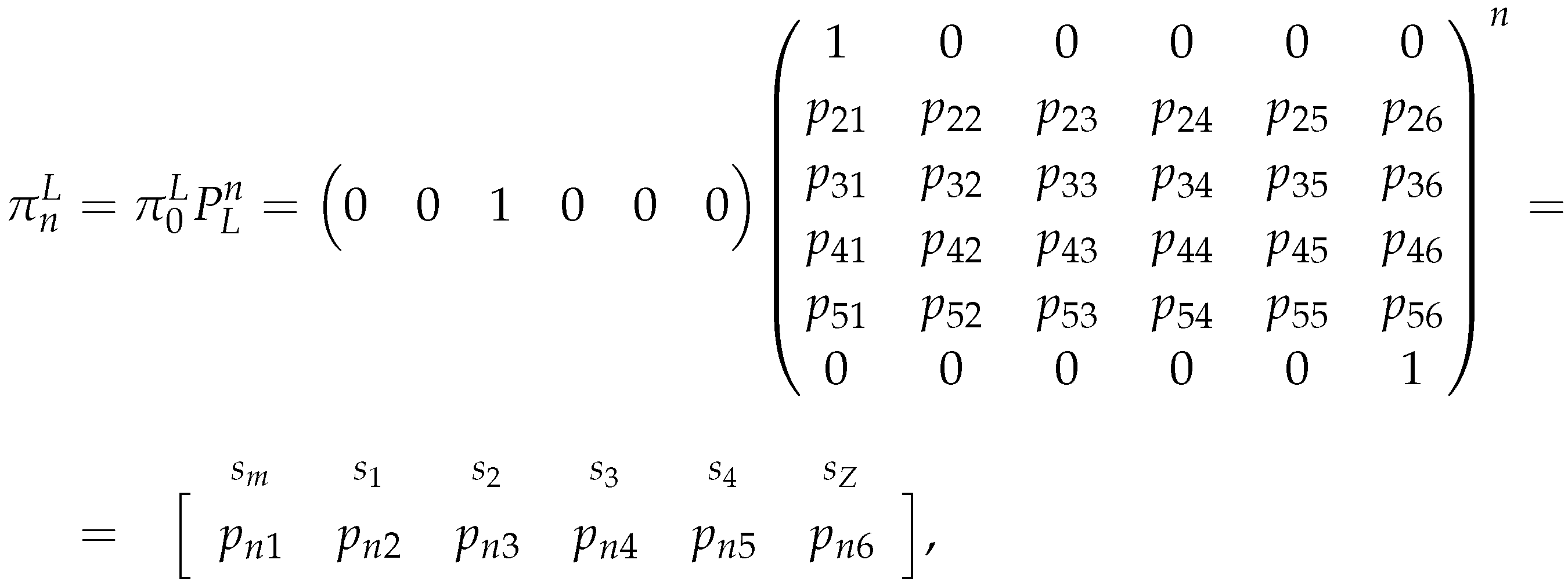
which, after the matrix multiplication, yields a

1 \times 6

vector

π_{n}

. And, its last entry is the probability of the chain being in state

s_{Z}

after n iterations, so our estimator for

p_{0}

is:

p_{0} \approx p_{n 6} .

Observe that we had the same issues in both estimators, because the chains were not irreducible, also we used the same number of iterations n (to determine the long-run estimator) in both chains, so that we can compare the obtained results from the different chains. Finally, we need to note that these estimators (for

p_{0}

and

p_{2}

) sum up to a value

\leq 1

, because, by Section 2.2, the theoretical probabilities that we are estimating have this property, and by the fact that we are under-estimating the market’s probabilities, since theoretically we should determine the long-run estimator by using infinite iterations (and not only n).

Remark 14.

Even though the used notations for both estimators are similar, the obtained estimated probabilities result from (n iterations of) different chains, so they represent different probabilities. Additionally, the estimator for

p_{1}

is simply

p_{1} = 1 - p_{0} - p_{2}

, for both cases.

So, with all of this, we can estimate the probabilities of the market playing a certain strategy and thus choose the speculator’s optimal strategy according to the previously presented financial game.

To finalize this section we will just pick up the dataset from the Example 26 (from the previous section) and compute the estimators for the market’s probabilities. For this, recall that the obtained transition matrix related to the chain where we assumed the More Risk strategy is:

(55)

The obtained transition matrix related to the chain where we assumed the Less Risk strategy is:

(56)

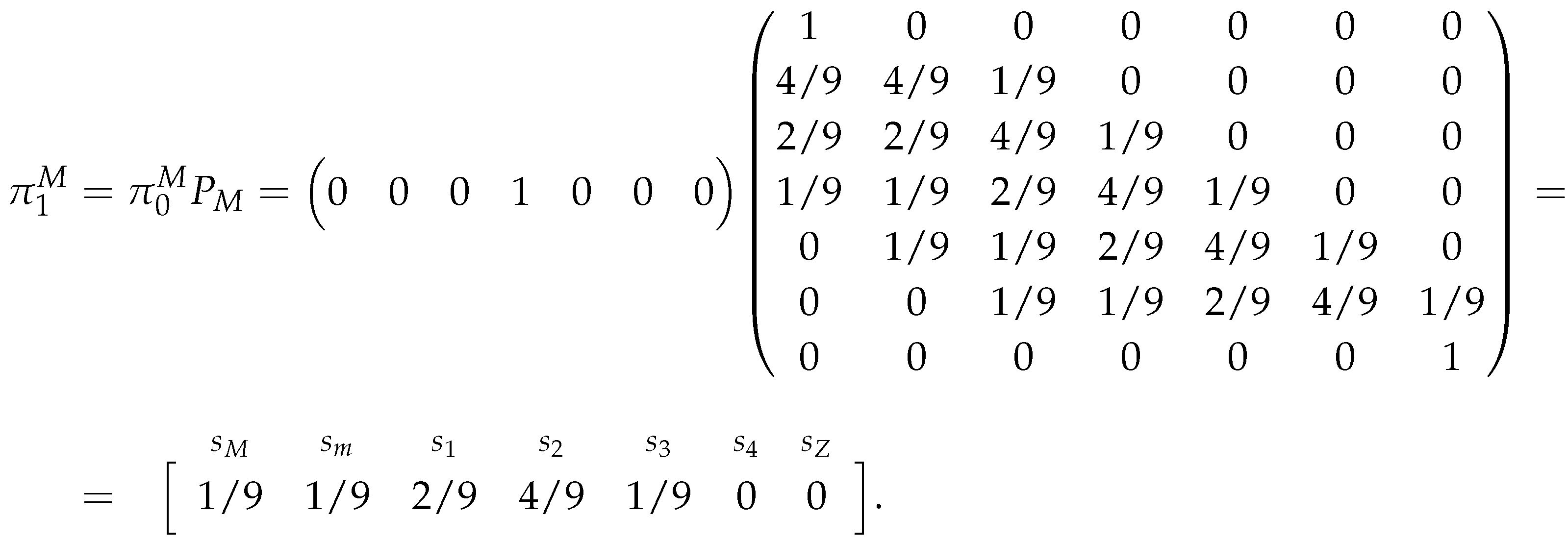
So, assuming

π_{0}^{M} = {(0, 0, 0, 1, 0, 0, 0)}^{T}

, we have that:

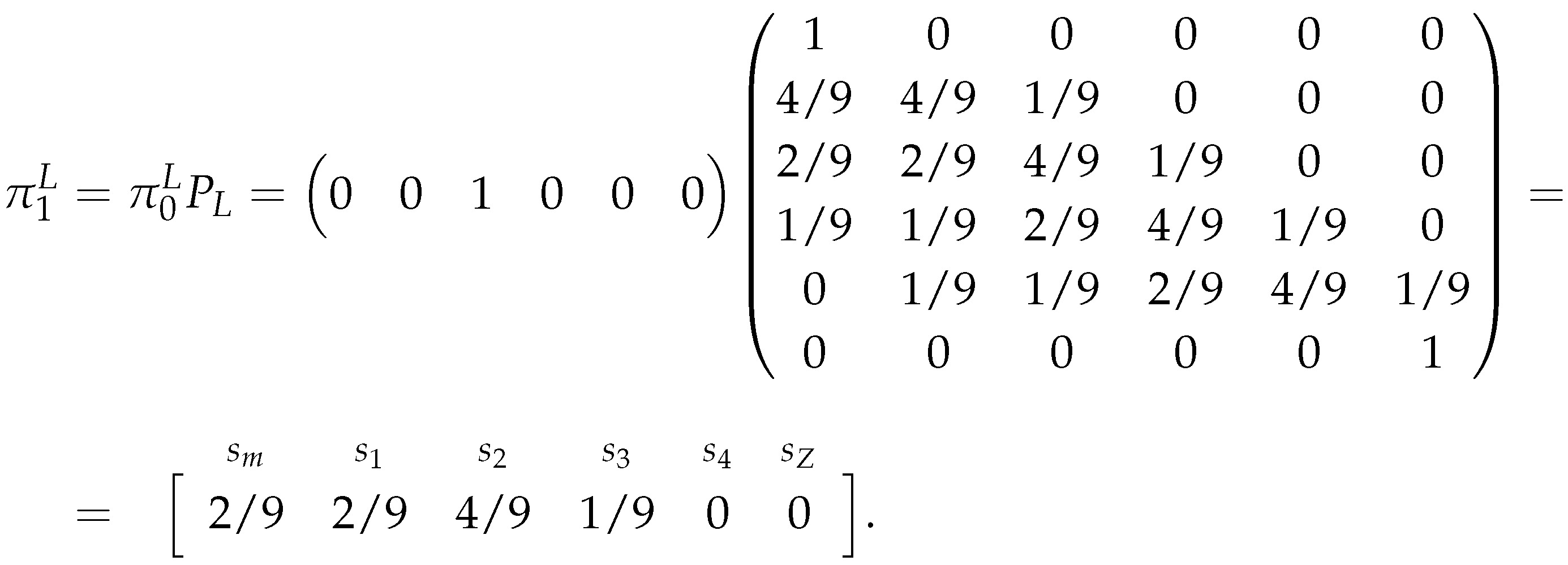
And with

π_{0}^{M} = {(0, 0, 0, 1, 0, 0, 0)}^{T}

we have:

So the one iteration estimators for the market’s probabilities, for this example, are:

\begin{matrix} p_{0} = 0 \\ p_{1} = 8 / 9 \approx 0.89 \\ p_{2} = 1 / 9 \approx 0.11 \end{matrix}

Regarding the long run estimator with

n = 10

iterations, we have that:

Remark 15.

Note that the presented values are rounded with two decimal cases.

So the long-run estimators for the market’s probabilities, for this example, are:

\begin{matrix} p_{0} = 0.01 \\ p_{1} = 0.09 \\ p_{2} = 0.9 \end{matrix}

Note that the estimated probabilities, in this example, change drastically from one estimator to the other, also they suggest that the market (as the iterations of the chain increase) is increasing its probability of choosing the Major Adversity strategy.

Table 6. Example 26’s game table for the financial market game.

		Speculator
			q	$1 - q$
			$R^{+}$	$R^{-}$
Market	$p_{0}$	$0_{A}$	9	9
	$p_{1}$	$m_{A}$	9	$- 6$
	$p_{2}$	$M_{A}$	$- 9$	$- 6$

To finalize, the previously presented game Table 2 related to the financial game, for this example, becomes:

These payoffs (or strategy thresholds) were obtained by applying the theory on Section 2.1 and considering the standard deviation of the transformed dataset (i.e., considering

α = 3

), where we obtained

w = 9

x = 6

and

y = 9

Now, with the one iteration estimators and considering the probability triangle (also presented in Section 2.1, but considering these new values), for this case, the speculator should choose to play the More Risk strategy, because:

p_{2} = 0.11 < \frac{w}{w + y} = 0.5 and \frac{p_{1}}{p_{2}} \approx 8.09 > \frac{y - x}{w + x} = 0.2 .

(57)

And, considering the long run estimator and the same probability triangle, the speculator should choose not to play, because:

p_{1} + p_{2} = 0.99 > = \frac{w}{w + y} = 0.5 and p_{2} = 0.9 > \frac{w}{w + y} = 0.5 .

(58)

Thus, as we can see the two estimators yield different strategies for the speculator to choose. All of this because the market "changes" its behavior as the iterations increase.

2.3. The SARIMA and GARCH Models

Now that we have discussed the specific game theoretical and Markov chains models that we will use, it is time to describe how we will use the SARIMA and GARCH models to predict the market’s behavior, and then compare the accuracy of the three approaches. However, we cannot simply apply the time series models to the raw dataset and make a prediction for the future value of the time series, because, in order to make the comparison of the models possible, we need to apply all the models to the same dataset and try to predict the same objects, which in our case means predicting the strategies that the market will choose. Thus, we will apply the time series models to the same percentage change transformed datasets that we have been using on the previous sections. So, if we make predictions based on these models, we obtain percentage change transformed predictions of the asset’s price (which is useful, but it is not our ultimate goal).

To obtain a prediction of the market’s strategy, firstly we will estimate the optimal time series models for the dataset. Then, using these estimated models, we will perform K simulations each with N observations, thus obtaining K simulations of percentage change prices for each of the models and each one starting on the last observation of the transformed dataset.

Remark 16.

All of this will be done with the aid of the R software, which we will elaborate further on Section 2.4.

Now, as in the previous sections, consider the speculator’s More Risk strategy thresholds in terms of the dataset’s standard deviation

α

the Profit Objective threshold: $s_{P} \geq 3 \cdot α$ ;
the More Risk threshold: $s_{R} \leq - 3 \cdot α$ .

Finally, for each of the K simulations, we need to check which of the thresholds was reached first, because the speculator will exit the trade (or the game) when one of these is reached. And with this we obtain the absolute frequencies of each of the thresholds, and also its relative frequencies if we divide by K.

Remark 17.

Note that, as we are performing simulations involving a model which includes a probability distribution, if we ran the same code several times, we would obtain different results after each run. However, these results will not have major differences between them.

Hence, we will estimate the probability of the market playing the Major Adversity strategy (

p_{2}

) with the relative frequency related to the More Risk threshold, and similarly the probability of the market playing the Zero Adversity strategy (

p_{0}

) with the relative frequency related to the Profit Objective threshold. Also, by default, the estimation for probability of the market playing the Minor Adversity strategy (

p_{1}

) is simply

1 - p_{2} - p_{0}

. Additionally, since we have the market’s probabilities, then we can choose the speculator’s optimal strategy according to the probability triangle presented in Section 2.1.2. But, before moving on, note that we need to determine these probabilities for both the SARIMA and the GARCH models, so we need to make an estimation for each of these models (but always using the same dataset), i.e., we need to perform K simulations for each model estimation and then determine the probabilities for each set of estimations. So, we will obtain two optimal strategies, one for each of the models.

Thus, for all the models presented so far (specifically, Markov Chain, SARIMA and GARCH), the speculator will obtain a optimal strategy for each of them, which is done by estimating the market’s probabilities (which may differ for each model) and then we will apply the same probability triangle for each set of probabilities.

2.4. Procedures

Now that we have all the necessary models and estimators, it is time to describe how we will use each model to choose the optimal strategy for a certain dataset. Also, we need to explain how we will check if the predictions were accurate and how accurate.

Consider an abstract dataset composed by strictly positive values, which will represent the price of a certain financial asset for

n + 1

consecutive iterations (it can be

n + 1

consecutive minutes, days,...). Since we worked with percentage change data in the game theoretical model, then we will apply the percentage change transformation to the dataset, obtaining a transformed dataset

C = {c_{1}, \dots, c_{n}}

composed with percentage changes of

n + 1

consecutive iterations. So, we will apply all of our models to this dataset C. Also, in order to check the accuracy of our models, we will split the dataset into training (

C_{1}

) and test (

C_{2}

) sets, where the training set will be composed by the first

80 %

of the observations and the remaining will belong to the test set. Thus, considering the set

C = {c_{1}, \dots, c_{n}}

, the training set will be

C_{1} = {c_{1}, \dots, c_{k}}

and the test set

C_{2} = {c_{k + 1}, \dots, c_{n}}

, for

k < n

The general procedure applied to a (transformed and divided) dataset C, consists on estimating the market’s probabilities for each of the models (Markov chains, SARIMA and GARCH), thus obtaining three "pairs" of probabilities, then we will use them to determine the speculator’s optimal strategy, also obtaining three optimal strategies. Afterwards, we will use the test set to check if the obtained strategies were accurate predictions for the current training set.

To accomplish this, consider the speculator’s More Risk strategy thresholds (as we did in the previous section) in terms of the dataset’s standard deviation

α

the Profit Objective threshold: $s_{P} = 3 α$ ;
the More Risk threshold: $s_{R} = - 3 α$ .

Then, using the test set, we will check which of the thresholds was reached first. So, this information together with the chosen optimal strategies, gives us the accuracy of the predictions, specifically:

considering that optimal chosen strategy was the More Risk strategy, then we will consider that strategy to be accurate if the first threshold to be reached in the test set was the Profit Objective threshold, otherwise the strategy will be considered to be not accurate;
considering that optimal chosen strategy was the Less Risk strategy, then we will consider that strategy to be accurate if the first threshold to be reached in the test set was the Profit Objective threshold, otherwise the strategy will be considered to be not accurate;
considering that optimal chosen strategy was the Do Not Play strategy, then we will consider that strategy to be accurate if the first threshold to be reached in the test set was the More Risk threshold, otherwise the strategy will be considered to be not accurate.

Note that the Less Risk threshold was not necessary to determine the accuracy of the strategies. Also, due the nature of the data, none of the thresholds may be reached, so, in this case, we will not consider the strategy to be accurate nor inaccurate. Hence, in this situation, we can decrease the thresholds and recalculate the optimal strategies, or we can just consider that the accuracy cannot be determined due to the nature of the data.

Finally, in order to have more samples to analyze, we will increase the training set by one observation and decrease the test set by one observation, thus obtaining the sets

C_{1} = {c_{1}, \dots, c_{k}, c_{k + 1}}

and

C_{2} = {c_{k + 2}, \dots, c_{n}}

. Then we will redo what we described before, but considering these new sets as training and test sets, respectively. Thus, we will obtain new accuracy data for the new optimal strategies.

To summarize, consider the transformed dataset

C = {c_{1}, \dots, c_{n}}

split between a training set

C_{1} = {c_{1}, \dots, c_{k}}

and a test set

C_{2} = {c_{k + 1}, \dots, c_{n}}

, then the procedure to be applied is:

Considering the training set $C_{1}$ :
- estimate the market’s probabilities using the Markov chains model and determine the optimal strategy for speculator using the game theoretical model;
- estimate the optimal SARIMA model, estimate the market’s probabilities using the model’s simulations and determine the optimal strategy for the speculator using the game theoretical model;
- estimate the optimal GARCH model, estimate the market’s probabilities using the model’s simulations and determine the optimal strategy for the speculator using the game theoretical model.
Considering the test set $C_{2}$ :
- check the accuracy of the three obtained optimal strategies, using the previously described method;
- store the accuracy results for each of the models.
Increase the training set $C_{1}$ by one observation and shorten the test set $C_{2}$ also by one observation, thus we will now consider the training set to be $C_{1} = {c_{1}, \dots, c_{k}, c_{k + 1}}$ and the test set to be $C_{2} = {c_{k + 2}, \dots, c_{n}}$ .
Perform all of the previous steps considering the "new" training and test sets, but end the procedure when the test set only has one observation remaining.

After applying this procedure, we need to analyze the obtained results, which we will do next.

3. Results

Now, we can put what was presented into practice with some real-time data from the financial markets, compare the models’ accuracy results and thus derive some conclusions from them.

Firstly, we will make our analysis for some controlled datasets, with the objective to check how the models perform in "well-behaved" scenarios, and then move on to datasets with daily and intraday data. But, before moving further, let us recall that a model is said to be accurate if the speculator’s obtained optimal strategies were the correct ones (when comparing to the test set) after the procedure described in Section 2.4 (from Chapter 2) ended. Likewise, the model is said to be inaccurate if the speculator’s obtained optimal strategies were the incorrect ones (when comparing to the test set) after the same procedure ended. However, if a model’s accuracy could not be determined (at a certain time) then it is said to have null accuracy. Additionally, we will also present (and analyze) the following characteristics obtained from applying the described procedures:

The percentage of times that the several models obtained the same strategies. This was done in order to check how often different approaches would lead to the same optimal strategies. Also, we will present these results regarding pairs of models, for instance we will present the percentage of times that the Markov chains and the SARIMA models obtained the same strategies.
The average time (in the same units as the corresponding dataset) that it took for the trade to close (in the test set), after a strategy was given. This average time was obtained by determining the number necessary iterations for the several test sets to reach one of the speculator’s thresholds.
The percentage of the speculator’s obtained strategies that were "Play Less Risk", "Play More Risk" and/or "Do Not Play".
We used the obtained strategies and entered a fictional market with an initial monetary value of 10000, where we only bought one item of each financial asset. This was done in order to see the profit that we would obtain if we entered a financial market and used the speculator’s obtained strategies (for each of the models) to enter (and then exit) a trade.

To facilitate the presentation, we will round all of the results up to two decimal cases, but, if needed to, we will display some results in scientific notation. Thus, the values that will be presented are approximations of the actual results.

Remark 18.

In order to make the text lighter, we will refer to the Markov chains model considering the one iteration estimator as the MC1 model, and to the Markov chains model considering the long-run estimator as the MCn model.

Finally, the following sections will be structured in the same manner, that is, a brief explanation of the dataset(s), followed by the presentation of each model’s obtained accuracy results (and related conclusions), ending with the analysis of some characteristics resultant from the models’ appliance.

3.1. Controlled Datasets

For this section, we will start by explaining how we constructed each dataset and make an overall analysis of the obtained results.

The first dataset was constructed with the purpose to check how the models perform in a "mild" Major Adversity scenario, i.e., the price of the asset will not always be decreasing but its trend will. And to obtain such a dataset we followed the presented steps until we obtained 1000 observations:

defined the first value of the dataset as 1000;
the second value of the dataset is just an increase of $3 %$ of the previous one;
the third value of the dataset is a decrease of $9 %$ of the previous one;
the even observations are obtained with an increase of $3 %$ of the previous value;
the odd observations are obtained with a decrease of $9 %$ of the previous value.

We constructed the dataset in this manner in order to mimic an event of Major Adversity, so for the models to "perform well" in this dataset, the speculator’s obtained optimal strategy must always be "Do Not Play", because the market, ultimately, is choosing to decrease the asset’s price in the long-run.

The second dataset was constructed with the purpose to check how the models perform in an "extreme" Major Adversity scenario, i.e., the price of the asset will always be decreasing. To obtain such a dataset, we just defined it as 1000 observations starting from 1000, always decreasing by

3 %

of the previous value and adding a random value from a standard normal distribution. We constructed the dataset in this manner in order to mimic an extreme event of Major Adversity. So, for the models to "perform well" in this dataset, the speculator’s obtained optimal strategy must always be "Do Not Play", because the market will always choose the Major Adversity strategy.

The third dataset was constructed with the purpose to check how the models perform in a "mild" Zero Adversity scenario, i.e., the price of the asset will not always be increasing but its trend will. And to obtain such a dataset we followed the presented steps until we obtained 1000 observations:

defined the first value of the dataset as 1000;
the second value of the dataset is just an decrease of $3 %$ of the previous one;
the third value of the dataset is a increase of $9 %$ of the previous one;
the even observations are obtained with a decrease of $3 %$ of the previous value;
the odd observations are obtained with an increase of $9 %$ of the previous value.

We constructed the dataset in this manner in order to mimic an event of Zero Adversity, so for the models to "perform well" in this dataset, the speculator’s obtained optimal strategy must either be "Play Less Risk" or "Play More Risk", because the market, ultimately, is choosing to increase the asset’s price in the long-run.

The last dataset was constructed with the purpose to check how the models perform in an "extreme" Zero Adversity scenario, i.e., the price of the asset will always be increasing. To obtain such a dataset, we just defined it as 1000 observations starting from 1000, always increasing by

3 %

of the previous value and adding a random value from a standard normal distribution. We constructed the dataset in this manner in order to mimic an extreme event of Zero Adversity. So, for the models to "perform well" in this dataset, the speculator’s obtained optimal strategy must always be "Play Less Risk" (or even "Play More Risk"), because the market will always choose the Zero Adversity strategy.

Now that we have explained how each dataset was constructed, we will make a global analysis of the obtained results for the controlled datasets (considering that

20 %

of the data belongs to the test set), obtaining:

The highest standard deviation of the transformed datasets was $α \approx 3$ (obtained in Datasets 1 and 3) and the lowest was $α \approx 0$ (in Dataset 2).
The MC1 model was $75 %$ more accurate then the other models, i.e., on 3 datasets this model had higher (or equal) accuracy results than all the other models. Also, the highest accuracy result was $100 %$ (obtained in Datasets 2 and 4), while the lowest was $0 %$ (on Dataset 1).
The MCn, SARIMA and GARCH models were $100 %$ more accurate then the other models. Additionally, the highest accuracy result was $100 %$ (obtained in Datasets 2 and 4), while the lowest was $98.5 %$ (on Dataset 3).

From these results we can see that the MCn, SARIMA and GARCH models are the models with the best accuracy results, which means that if the speculator used these models (for these datasets), he/she would obtain more strategies that would result in a profit (or at least a smaller loss). Consequently, the MC1 model obtained the worst accuracy results. Also we need to note that the lowest accuracy results were always obtained in the same datasets, while the highest was almost always in the same one.

Finally,

50 %

of the datasets presented no null accuracy results for all the models, meaning that the thresholds were always reached in all of the test sets. In Dataset 1,

0.5 %

of the models resulted in null accuracy results, which was the same for all the models. While this percentage was

1.5 %

for Dataset 3.

Moving to the obtained characteristics (which resulted from the explained procedures) for these controlled datasets were:

The percentage of times that the several models obtained the same strategies:

-

The MCn model fully coincided in all the datasets with the time series models, i.e., in all the dataset these models always resulted in the same strategies

-

The MC1 model fully coincided in $50 %$ of the datasets with all the other models, but on the other hand, it never coincided with any model in the other datasets.
The average time (in iterations) for all of the datasets was the same across all of the models. Also, the highest average time was 3.475 iterations (in Dataset 3) and the lowest was 1 iteration (on Datasets 2 and 4).
The percentage of the speculator’s obtained strategies for each of the models was:

-

For the MC1 model:

*

in $50 %$ of the datasets always chose the More Risk strategy;

*

in $25 %$ of the datasets always chose the Less Risk strategy;

*

in $25 %$ of the datasets always chose the Not Play strategy.

-

For the MCn, SARIMA and GARCH models:

*

in $50 %$ of the datasets always chose the Less Risk strategy;

*

in $50 %$ of the datasets always chose the Not Play strategy.

The obtained possible profits using each model were:

-

For the MC1 model:

*

negative in $25 %$ of the datasets, null in $25 %$ and positive in the remaining ones;

*

the lowest profit (or highest loss) was in Dataset 1;

*

the highest profit was in Dataset 3.

-

For the MCn, SARIMA and GARCH models:

*

null in $50 %$ of the datasets and positive in the remaining datasets;

*

the lowest profit (or highest loss) was in Datasets 1 and 2;

*

the highest profit was in Dataset 3.

As it was said before, the MCn, SARIMA and GARCH models fully coincided between them, in terms of accuracy results and chosen strategies. But, on the other hand, the MC1 model never coincided with all the other models in

50 %

of the datasets.

The MC1 model in

50 %

of the datasets always chose the More Risk strategy, and then switched between all the strategies in the remaining datasets. Meanwhile, the other models always chose the Less Risk strategy in

50 %

of the datasets, and then the Not play strategy on the other datasets.

In terms of possible profits, the MCn, SARIMA and GARCH models obtained positive profits in

50 %

of the datasets and null profits on the other ones, while the MC1 model obtained negative profits in

25 %

of the datasets, null profits in

25 %

and the remaining were positive.

From all of these results, we can see that the MCn, SARIMA and GARCH models obtained better accuracy and profits results, because they chose the expected optimal strategies for each of the datasets. While the MC1 model was the worst in all of the same aspects.

Finally, the average time it took the models to reach a threshold always coincided between models and its range was approximately from 1 to 3 iterations. Also, we need to note that both the highest and lowest profits were always obtained in the same datasets.

3.2. Daily Datasets

For this section, we will analyze datasets which are only composed with daily closing prices of several financial assets, this means that we are going to analyze the assets’ prices at the end of each day (specifically, at the closing of the financial market).

We applied our models to 100 different datasets, but we will not analyze each of them, rather we will make a global analysis of the results. Also, note that whenever we refer to a specific dataset, we are actually referring to the price data that we obtained for a certain financial asset. Additionally, all the datasets have exactly 1000 observations of the closing price at the end of the day.

Thus, after applying our models to these datasets, considering that

20 %

of the data belongs to the test set, we obtained that:

The highest standard deviation of the transformed datasets was $α \approx 3.44$ (obtained in dataset TNXP) and the lowest was $α \approx 0$ (in dataset PSON).
The MC1 model was $41 %$ more accurate then the other models, i.e., on 41 datasets this model had higher (or equal) accuracy results than all the other models. Also, the highest accuracy result was $66.5 %$ (obtained in dataset AAPL), while the lowest was $33.5 %$ (on dataset TNXP).
The MCn model was $50 %$ more accurate then the other models. And, the highest accuracy result was $66.5 %$ (obtained in datasets AAPL and TNXP), while the lowest was $34.5 %$ (on dataset NOS).
The SARIMA model was $42 %$ more accurate then the other models. And, the highest accuracy result was $66.5 %$ (obtained in dataset AAPL), while the lowest was $35 %$ (on dataset GFS).
The GARCH model was $40 %$ more accurate then the other models. And, the highest accuracy result was $66.5 %$ (obtained in dataset AAPL), while the lowest was $35.5 %$ (on dataset NOS).

From these results we can see that the MCn model is the one with the best accuracy results, which means that if the speculator used this model (for these datasets), he/she would obtain more strategies that would result in a profit (or at least a smaller loss). Additionally, the MC1, SARIMA and GARCH models obtained very similar accuracy results.

Regarding the time series models, the SARIMA model obtained slightly higher accuracy results than the GARCH model, which is the opposite of what was expected, since the GARCH models were specifically developed for this kind of data, as such it would be expected for them to perform better in terms of accuracy.

Finally, the obtained null accuracy results were the same across all the models and were almost always zero, also the highest percentage of null models was

6 %

(obtained in dataset TWTR). Additionally, we need to note that the highest accuracy results were always obtained in the same dataset.

The obtained characteristics (which resulted from the explained procedures) for these datasets were:

The percentage of times that the several models obtained the same strategies:

-

The Markov chains models fully coincided between them in $81 %$ of the datasets, i.e., in 81 datasets these two models always resulted in the same strategies. Also they never coincided in $5 %$ of the datasets and, on the other datasets, the percentage of coinciding models ranged from $2 %$ to $99 %$ .

-

The MC1 model never coincided (in all the datasets) with the time series models.

-

The MCn model never coincided in $81 %$ of the datasets with the SARIMA model and, on the other datasets, the percentage of coinciding models ranged from $1 %$ to $98 %$ .

-

The MCn model never coincided in $82 %$ of the datasets with the GARCH model and, on the other datasets, the percentage of coinciding models ranged from $0.5 %$ to $98.5 %$ .

-

The SARIMA model fully coincided with the GARCH model in $6 %$ of the datasets and, on the other datasets, the percentage of coinciding models ranged from $51.5 %$ to $99.5 %$ .

The average time (in days) for all the datasets was the same across all the models. Also, the highest average time was 9.35 days (in dataset GFS) and the lowest was 1.015 days (on dataset PSON).
The percentage of the speculator’s obtained strategies for each of the models was:

-

The MC1 model always chose to play the More Risk strategy on all of the datasets.

-

For the MCn model:

*

in $81 %$ of the datasets always chose the More Risk strategy;

*

in $1 %$ of the datasets always chose the Less Risk strategy;

*

in $4 %$ of the datasets always chose the Not Play strategy;

*

in $1 %$ of the datasets chose between the play More Risk and Less Risk strategies;

*

in $13 %$ of the datasets only chose between the More Risk and Not Play strategies.

-

For the SARIMA model:

*

in $5 %$ of the datasets always chose the Less Risk strategy;

*

in none of the datasets always chose the More Risk and Not Play strategies;

*

in the remaining datasets only chose between the Less Risk and Not Play strategies. Also, the percentage of times the Less Risk strategy was chosen (instead of the Not Play strategy) is less than $50 %$ in only $3 %$ of all the datasets.

-

For the GARCH model:

*

in $26 %$ of the datasets always chose the Less Risk strategy;

*

in none of the datasets always chose the More Risk and Not Play strategies;

*

in the remaining datasets only chose between the Less Risk and Not Play strategies. Also, the percentage of times the Less Risk strategy was chosen (instead of the Not Play strategy) is less than $50 %$ in only $1 %$ of all the datasets.
The obtained possible profits using each model were:

-

For the MC1 model:

*

negative in $18 %$ of the datasets and positive in the remaining datasets;

*

the lowest profit (or highest loss) was in dataset CCL;

*

the highest profit was in dataset AZN.

-

For the MCn model:

*

negative in $16 %$ of the datasets, null in $4 %$ of the datasets and positive in the remaining datasets;

*

the lowest profit (or highest loss) was in dataset CCL;

*

the highest profit was in dataset AZN.

-

For the SARIMA model:

*

negative in $25 %$ of the datasets and positive in the remaining datasets;

*

the lowest profit (or highest loss) was in dataset CCL;

*

the highest profit was in dataset AVV.

-

For the GARCH model:

*

negative in $19 %$ of the datasets and positive in the remaining datasets;

*

the lowest profit (or highest loss) was in dataset CCL;

*

the highest profit was in dataset AZN.

From the first item we can see that no model fully coincided in terms of chosen strategies with another one, but, on the other hand, the MC1 model never coincided with the time series models (SARIMA and GARCH), similarly the MCn model almost never coincided with the time series models. Also, the Markov chains models almost always coincided between them. Regarding the time series models, they almost always coincided between them, even though they only fully coincided in

6 %

of the datasets.

The MC1 model always chose the More Risk strategy across all of the datasets, while this only happened in

81 %

of the datasets for the MCn model. But, unlike the Markov chains models, the time series models never chose the More Risk strategy.

From all of these results, we can see that the MCn model performed better both in terms of accuracy results and of possible profits. Meanwhile, the MC1 model performed similarly to the time series models, both in terms of accuracy results and of possible profits. Also, regarding the time series models, the SARIMA model had slightly higher accuracy results than the GARCH model, however it had the highest percentage of unprofitable datasets.

Finally, the average time it took the models to reach a threshold always coincided between models and its range was from approximately a day to two weeks (each week in the financial markets is composed by five days). Also, we need to note that the lowest profit was always obtained in the same dataset, while the highest one was almost always obtained in the same one.

3.3. Intraday Datasets

For this section, we will analyze datasets which are only composed with 1000 observations of intraday closing prices of several financial assets, this means that we are going to analyze the assets’ prices at the end of each minute for several days. Also, we applied our models to 100 different datasets, but we will not analyze each of them, rather we will make a global analysis of the results. Also, note that whenever we refer to a specific dataset, we are actually referring to the price data that we obtained for a certain financial asset.

Thus, after applying our models to these datasets, considering that

20 %

of the data belongs to the test set, we obtained that:

The highest standard deviation of the transformed datasets was $α \approx 2.13$ (obtained in dataset TNXP), also this value was the only value for the standard deviation greater than 1. Furthermore, all the other values for the standard deviation were smaller than 0.4, where the lowest was $α \approx 0$ (in dataset Z).
The MC1 was $27 %$ more accurate then the other models, i.e., on 27 datasets this model had higher (or equal) accuracy results than all the other models. Also, the highest accuracy result was $68.5 %$ (obtained in dataset NOS), while the lowest was $0.5 %$ (on dataset TWTR).
The MCn model was $43 %$ more accurate then the other models. And, the highest accuracy result was $78.5 %$ (obtained in dataset FCX), while the lowest was $0.5 %$ (on dataset TWTR).
The SARIMA model was $43 %$ more accurate then the other models. And, the highest accuracy result was $74 %$ (obtained in dataset BCP), while the lowest was $2.5 %$ (on dataset TWTR).
The GARCH model was $33 %$ more accurate then the other models. And, the highest accuracy result was $67.5 %$ (obtained in dataset O), while the lowest was $14 %$ (on dataset TWTR).

From these results we can see that the MCn and SARIMA models were the ones with the best accuracy results, which means that if the speculator used one of these models (for these datasets), he/she would obtain more strategies that would result in a profit (or at least a smaller loss). Meanwhile, the MC1 model was the one with the lowest accuracy results.

Regarding the time series models, the SARIMA model obtained higher accuracy results than the GARCH model, which is the opposite of what was expected, since the GARCH models were specifically developed for this kind of data.

Finally, the obtained null accuracy results were the same across all the models and were almost always zero, where the highest percentage of null models was

12.5 %

(obtained in dataset TWTR). Also, we need to note that the smallest accuracy results were always obtained in the same dataset.

The obtained characteristics (which resulted from the explained procedures) for these controlled datasets were:

The percentage of times that the several models obtained the same strategies:

-

The Markov chains models fully coincided between them in $61 %$ of the datasets, i.e., in 61 datasets these two models always resulted in the same strategies. Also, they never coincided in $17 %$ of the datasets and, on the other datasets, the percentage of coinciding models ranged from $1 %$ to $98.5 %$ .

-

The MC1 model never coincided in all the datasets with the time series models.

-

The MCn model fully coincided with the SARIMA model in $1 %$ of the datasets, never coincided in $67 %$ of the datasets and, on the other datasets, the percentage of coinciding models ranged from $1 %$ to $87.5 %$ .

-

The MCn model never coincided with the GARCH model in $76 %$ of the datasets and, on the other datasets, the percentage of coinciding models ranged from $0.5 %$ to $95.5 %$ .

-

The SARIMA model fully coincided with the GARCH model in $4 %$ of the datasets and, on the other datasets, the percentage of coinciding models ranged from $12.5 %$ to $99.5 %$ .
The average time (in minutes) for all the datasets was the same across all the models. And, the highest average time was 52.56 minutes (in dataset TWTR), while the lowest was 1.035 minutes (on dataset Z).
The percentage of the speculator’s obtained strategies for each of the models was:

-

The MC1 model always chose to play the More Risk strategy on all of the datasets.

-

For the MCn model:

*

in $61 %$ of the datasets always chose the More Risk strategy;

*

in $1 %$ of the datasets always chose the Less Risk strategy;

*

in $16 %$ of the datasets always chose the Not Play strategy;

*

in $22 %$ of the datasets only chose between the More Risk and Not Play strategies.

-

For the SARIMA model:

*

in $5 %$ of the datasets always chose the Less Risk strategy;

*

in none of the datasets always chose the More Risk and Not Play strategies;

*

in the remaining datasets only chose between the Less Risk and Not Play strategies. Also, the percentage of times the Less Risk strategy was chosen (instead of the Not Play strategy) is less than $50 %$ in only $7 %$ of all the datasets.

-

For the GARCH model:

*

in $27 %$ of the datasets always chose the Less Risk strategy;

*

in none of the datasets always chose the More Risk;

*

in the remaining datasets, only chose between the Less Risk and Not Play strategies. Also, the percentage of times the Less Risk strategy was chosen (instead of the Not Play strategy) is less than $50 %$ in only $3 %$ of all the datasets.
The obtained profits using each model were:

-

For the MC1 model:

*

negative in $41 %$ of the datasets and positive in the remaining datasets;

*

the lowest profit (or highest loss) was in dataset RB;

*

the highest profit was in dataset AZN.

-

For the MCn model:

*

negative in $37 %$ of the datasets, null in $16 %$ and positive in the remaining datasets;

*

the lowest profit (or highest loss) was in dataset RB;

*

the highest profit was in dataset AHT.

-

For the SARIMA model:

*

negative in $40 %$ of the datasets and positive in the remaining datasets;

*

the lowest profit (or highest loss) was in dataset RB;

*

the highest profit was in dataset AZN.

-

For the GARCH model:

*

negative in $43 %$ of the datasets and positive in the remaining datasets;

*

the lowest profit (or highest loss) was in dataset RB;

*

the highest profit was in dataset AZN.

From the first item we can see that no model fully coincided in terms of chosen strategies with another one, but the MC1 model never coincided with the time series models (SARIMA and GARCH), and the MCn model almost never coincided with the time series models. Also, the Markov chains models almost always coincided between them. Similarly, the time series models almost always coincided between them, even though they only fully coincided in

4 %

of the datasets.

The MC1 model always chose the More Risk strategy across all the datasets, while this only happened in

61 %

of the datasets for the MCn model. But, unlike the Markov chains models, the time series models never chose the More Risk strategy.

The average time it took the models to reach a threshold always coincided between models and its range was from approximately 1 to 53 minutes. Also, the lowest profit was always obtained in the same dataset, while the highest was almost always obtained in the same one.

Finally, from all of these results, we can see that the MCn and SARIMA models were the ones with the best accuracy results, however, the MCn model had the lowest percentage of unprofitable datasets and was a model which resulted in all kinds of strategies. Additionally, regarding the time series models, the SARIMA model had better accuracy and profit results than the GARCH model.

4. Conclusions

Now that we have all the results for all the datasets, we can make a summary of what we obtained and then withdraw some conclusions from it.

Firstly, from all the obtained results, we can note that the lowest standard deviation of the transformed datasets was

α \approx 0

, while the highest was

α \approx 3

. Also, we need to note that, in the Intraday datasets,

99 %

of the transformed datasets had a standard deviation lower than

0.4

Regarding the obtained accuracy results for the models, we can see that the MCn model obtained the best accuracy results for each type of datasets (Controlled, Daily and Intraday), but on the Controlled datasets it tied with the time series models, while this happened with the SARIMA model in the Intraday datasets. About the maximum and minimum accuracy results, we obtained that:

for the Controlled datasets, the lowest accuracy result was almost always obtained in the same dataset, while the highest was always obtained in the same one;
for the Daily datasets, only the highest accuracy result was always obtained in the same dataset;
for the Intraday datasets, only the lowest accuracy result was always obtained in the same dataset.

Additionally, in all of the datasets both the null accuracy results and the average closing times were the same across the models. However, we need to note that, in terms of maximum results, the intraday datasets resulted in higher null results and higher average closing times.

For the percentage of equal strategies across the models we obtained that:

For the controlled datasets, the MCn model always coincided with the time series models. Meanwhile, the MC1 model fully coincided with the other models in $50 %$ of the datasets, whilst it never coincided in the other datasets.
For both the daily and intraday datasets, the Markov chains models almost always coincided between them. But the MC1 model never coincided with the time series models, and, consequently, the MCn model almost never coincided with the time series models. Regarding the time series models, they almost always had a high percentage of coinciding strategies between them, but they almost never fully coincided between them.

Now, regarding the percentage of chosen strategies for each of the models we obtained that:

For the controlled datasets, the MC1 model almost always chose the More Risk strategy (sometimes switching to the other strategies), while the other models chose between the Less Risk and Not Play strategies.
For both the daily and intraday datasets: the MC1 model always chose the More Risk strategy; the MCn model almost always chose the More Risk strategy, but it also chose between the other strategies; the time series models chose between the Less Risk and Not Play strategies.

Finally, regarding the obtained possible profits resulting from applying the different models we can see that the MCn model obtained the least percentage of unprofitable datasets for each type of datasets, but on the Controlled datasets it tied with the time series models, on the other hand, the MC1 model obtained the highest percentage of strictly positive profits in the Daily datasets, while the same happened for the Intraday datasets with the SARIMA model. About the maximum and minimum obtained possible profits, we have that:

for the Controlled datasets, the lowest and highest possible profits were always obtained in the same datasets;
for both the Daily and Intraday datasets, the lowest possible profit was always obtained in the same dataset (CCL and RB, respectively) and the highest was almost always obtained in the same one (AZN for both types).

Thus, gathering all these results, we can see that the Markov chains model (considering the long-run estimator) behaved better both in terms of accuracy and possible profits, than the other models, additionally, this model resulted in all kinds of strategies, unlike all the other models. So, with the Markov chains model (considering the long-run estimator), we obtained better results than all the other presented models.

Finally, the game theoretical model that we used as the decision model to make predictions (and to buy and sell financial assets) is a useful and accurate tool (both for the Markov chains models and the time series models), because it gives us an optimal strategy chosen in terms of these market probabilities, also these strategies are the same as the ones commonly used by the markets’ investors (and speculators). So, instead of directly predicting a financial asset’s price (and then acting upon this predictions), we can obtain a probabilistic model that lets us see how the financial markets behaved and where they may be going in terms of the assets’ prices.

4.1. Future Work

From the presented theory and subsequently results, a number of possible extensions can be made, such as:

create a new decision model that incorporates both the Markov chains and time series models;
add more classes to the Markov chains model, add more strategies to the game theoretical model and/or alter the existing classes/strategies;
study on how these models can be adapted to all kinds of data.

Also, we can study the possible relationships between the volatility, type and/or length of the datasets to:

the obtained optimal model (both in terms of accuracy and possible profit results);
the obtained values for the accuracy and possible profit results;
the standard deviations, the average closing time and the percentage of null models.

All of this should be studied in order to better model and predict the financial markets, and then extend to all kinds of data.

Author Contributions

This work is financed by: National Funds through the Portuguese funding agency, FCT - Fundação para a Ciência e a Tecnologia, within project LA/P/0063/2020; CMUP - Centro de Matemática da Universidade do Porto.

Institutional Review Board Statement

Not applicable.

Informed Consent Statement

Not applicable.

Data Availability Statement

The data presented in this study are openly available in https://www.kaggle.com/jfcf0802/daily-and-intraday-stock-data.

Conflicts of Interest

The authors declare no conflict of interest.

References

McDonald, J.B. Probability Distributions for Financial Models. Handbook of Statistics 1996, 14, 427–461. [Google Scholar]
Jackwerth, J.C.; Rubinstein, M. Recovering Probability Distributions from Option Prices. The Journal of Finance 1996, 51, 1661. [Google Scholar] [CrossRef]
Errunza, V.R.; Losq, E. The Behavior of Stock Prices on LDC Markets. Journal of Banking and Finance 1985, 9, 561–575. [Google Scholar] [CrossRef]
Mandelbrot, B.; Taylor, H.M. On the Distribution of Stock Price Differences. Operations Research 1967, 15, 1057–1062. [Google Scholar] [CrossRef]
Pishro-Nik, H. Introduction to Probability, Statistics, and Random Processes; Kappa Research, 2014.
Stewart, J. Calculus, 8 ed.; Cengage Learning, 2016.
McMillan, L.G. Options as a Strategic Investment, 4 ed.; Prentice Hall Press, 2001.
Murphy, J.E. Stock Market Probability: How to Improve the Odds of Making Better Investment Decisions; Probus Publishing, 1988.
Box, G.; Jenkins, G. Time Series Analysis, Forecasting and Control; Holden-Day, 1970.
Hipel, K.; McLeod, A. Time Series Modelling of Water Resources and Environmental Systems; Elsevier, 1994.
Gottlieb, G.; Kalay, A. Implications of the Discreteness of Observed Stock Prices. The Journal of Finance 1965, 11, 135–153. [CrossRef]
Scott, J.; Stumpp, M.; Xu, P. Overconfidence Bias in International Stock Prices. The Journal of Portfolio Management 2003, pp. 80–89.
Royal, J.; Arielle, O. What is the Average Stock Market Return?, 2020. [Online; accessed 24-April-2020].
Hume, D. A Treatise of Human Nature; 1739.
Hardin, G. The Tragedy of the Commons. Science 1968, 162, 1243–48.
Luce, R.D.; Raiffa, H. Games and Decisions; John Wiley & Sons, 1957.
Wald, A. Statistical Decision Functions; John Wiley & Sons, 1950.
Cournot, A. Researches into the Mathematical Principles of the Theory of Wealth; 1897.
Nash, J. Equilibrium Points in n-Person Games. Proceedings of the National Academy of Sciences 1950, 36, 48–49. [CrossRef]
Harsanyi, J. Games with Randomly Distributed Payoffs: A New Rationale for Mixed Strategy Equilibrium Points. International Journal of Game Theory 1973, 2, 1–23. [CrossRef]
Aumann, R. Subjectivity and Correlation in Randomized Strategies. Journal of Mathematical Economics 1974, 1, 67–96.
Aumann, R. Agreeing to Disagree. Annals of Statistics 1976, 4, 1236–1239.
Farber, H. An Analysis of Final-Offer Arbitration. Journal of Conflict Resolution 1980, 35, 683–705. [CrossRef]
Bertrand, J. Théorie Mathématique de la Richesse Sociale. Journal des Savants 1883, pp. 499–508.
Pearce, D. Rationalize Strategic Behavior and the Problem of Perfection. Econometrica 1984, 52, 1029–50.
Szép, J.; Forgó, F. Introduction to the Theory of Games; D. Reidel Publishing Company, 1985.
Fudenberg, D.; Tirole, J. Game Theory; The MIT Press, 1991.
Gibbons, R. A Primer in Game Theory; Pearson Education, 1992.
Biswas, T. Decision-Making Under Uncertainty; MAcMillan Press Ltd, 1997.
Kemeny, J.; Shell, J. Finite Markov Chains; Van Nostrand Company, 1960.
Bowerman, B.L. Nonstationary Markov decision processes and related topics in nonstationary Markov chains. Retrospective theses and dissertations. 6327, Iowa State University, Iowa, USA, 1974.
Fismen, M. Exact Simulation Using Markov Chains. Diploma-thesis (master-thesis) in statistics, Department of Mathematical Sciences, The Norwegian University of Science and Technology, Trondheim, Norway, 1997.
Welton, N.; Ades, A. Estimation of Markov Chain Transition Probabilities and Rates from Fully and Partially Observed Data: Uncertainty Propagation, Evidence Synthesis, and Model Calibration. MRC Health Services Research Collaboration 2005. [CrossRef]
Fette, B. Cognitive Radio Technology, 2 ed.; Academic Press, 2009.
Stewart, W.J. Probability, Markov chains, queues and simulation, 1 ed.; Princeton University Press, 2009.
Himmelmann, S.; www.linhi.com. HMM: HMM - Hidden Markov Models. R package version 1.0 2010.
Jackson, C.H. Multi-State Models for Panel Data: The msm Package for R. Journal of Statistical Software 2011, 38, 1–29. [CrossRef]
Wreede, L.; Fiocco, M.; Putter, H. mstate: An R Package for the Analysis of Competing Risks and Multi-State Models. Journal of Statistical Software 2011, 38, 1–30. [CrossRef]
Kobayashi, H.; Mark, B.L.; Turin, W. Probability, Random Processes and Statistical Analysis; Cambridge University Press, 2012.
Geyer, C.J.; Johnson, L..T. mcmc: Markov Chain Monte Carlo. R package version 0.9-2 2013.
Spedicato, G.A.; Kang, T.S.; Yalamanchi, S.B.; Yadav, D.; Cordón, I. The markovchain Package: A Package for Easily Handling Discrete Markov Chains in R. The R Journal 2017.
Box, G.; Jenkins, G. Time Series Analysis, Forecasting and Control; Holden-Day, 1976.
Engle, R.F. Autoregressive conditional heteroscedasticity with estimates of the variance of United Kingdom inflation. Econometrica 1982, 50, 987–1007. [CrossRef]
Bollerslev, T. Generalized autoregressive conditional heteroscedasticity. J. Econ. 1986, 31, 307–327. [CrossRef]
Hamilton, J.D. Time Series Analysis; Princeton University Press, 1994.
Box, G.; G.Jenkins.; Reinsel, G. Time Series Analysis, Forecasting and Control; Wiley, 2008.
Hyndman, R.; Khandakar, Y. Automatic time series forecasting: The forecast package for R. Journal of Statistical Software 2008, 27, 1–22. [CrossRef]
Shumway, R.H.; Stoffer, D.S. Time Series Analysis and Its Applications, 3 ed.; Springer Texts in Statistics, Springer, 2011.
Brockwell, P.; Davis, R. Introduction to Time Series and Forecasting, 3 ed.; Springer Texts in Statistics, Springer, 2016.
Shelton, R.B. Gaming the Market; Wiley Trading Advantage, John Wiley & Sons, 1997.

Figure 1. AAPL Daily Closing Price from 22/01/2016 to 10/01/2020

Figure 2. AAPL Intraday Closing Price from 03/02/2020 09:31 to 07/02/2020 16:00

Figure 3. GALP Daily Closing Price from 17/03/2016 to 13/02/2020

Figure 4. GALP Intraday Closing Price from 11/02/2020 04:00 to 17/02/2020 11:29

Figure 12. The probability triangle with all the analyzes done so far, which is divided into three regions: "Play Less Risk", "Play More Risk" and "Do Not Play".

Figure 13. The Markov Chain where we assume that the speculator chose to play the More Risk strategy.

Figure 14. The Markov Chain where we assume that the speculator chose to play the Less Risk strategy.

Disclaimer/Publisher’s Note: The statements, opinions and data contained in all publications are solely those of the individual author(s) and contributor(s) and not of MDPI and/or the editor(s). MDPI and/or the editor(s) disclaim responsibility for any injury to people or property resulting from any ideas, methods, instructions or products referred to in the content.

© 2024 by the authors. Licensee MDPI, Basel, Switzerland. This article is an open access article distributed under the terms and conditions of the Creative Commons Attribution (CC BY) license (http://creativecommons.org/licenses/by/4.0/).

Copyright: This open access article is published under a Creative Commons CC BY 4.0 license, which permit the free download, distribution, and reuse, provided that the author and preprint are cited in any reuse.

MDPI Initiatives

Important Links

Choose an area of interest and we will send you notifications of new preprints at your preferred frequency.

Disclaimer

Game Theory for Predicting Stocks’ Closing Prices

Abstract

1. Introduction

2. Models

2.1. The Game Theoretical Model

2.1.1. The Financial Game

2.1.2. The Probability Triangle

2.2. The Markov Chains Model

2.2.1. Defining the Markov Chains

2.2.2. Estimation of the Transition Probabilities

2.2.3. Estimating the Market’s Probabilities

2.3. The SARIMA and GARCH Models

2.4. Procedures

3. Results

3.1. Controlled Datasets

3.2. Daily Datasets

3.3. Intraday Datasets

4. Conclusions

4.1. Future Work

Author Contributions

Institutional Review Board Statement

Informed Consent Statement

Data Availability Statement

Conflicts of Interest

References

MDPI Initiatives

Important Links

Subscribe