Augmented Feature Diffusion on Sparsely Sampled Subgraph

Preprint

Article

Augmented Feature Diffusion on Sparsely Sampled Subgraph

Altmetrics

Downloads

128

Views

Comments

A peer-reviewed article of this preprint also exists.

This version is not peer-reviewed

Submitted:

18 July 2024

Posted:

22 July 2024

You are already at the latest version

Alerts

Abstract

Link prediction is a fundamental problem in graphs. Currently, SubGraph Representation Learning (SGRL) methods provide state-of-the-art solutions for link prediction by transforming the task into a graph classification problem. However, existing SGRL solutions suffer from high computational costs and lack scalability. In this paper, we propose a novel SGRL framework called Augmented Feature Diffusion on Sparsely Sampled Subgraph (AFD3S). The AFD3S first uses a conditional variational autoencoder to augment the local features of the input graph, effectively improving the expressive ability of downstream Graph Neural Networks. Then, based on a random walk strategy, sparsely sampled subgraphs are obtained from the target node pairs, reducing computational and storage overhead. Graph diffusion is then performed on the sampled subgraph to achieve specific weighting. Finally, the diffusion matrix of the subgraph and its augmented feature matrix are used for feature diffusion to obtain operator-level node representations as inputs for the SGRL-based link prediction. Feature diffusion effectively simulates the message-passing process, simplifying subgraph representation learning, thus accelerating the training and inference speed of subgraph learning. Our proposed AFD3S achieves optimal prediction performance on several benchmark datasets, with significantly reduced storage and computational costs.

Keywords:

Subject: Computer Science and Mathematics - Artificial Intelligence and Machine Learning

1. Introduction

The application of complex networks is becoming increasingly widespread in various fields [1], such as social networks [2,3,4], biological networks [5,6], transportation networks [7] and video processing tasks [8,9,10,11,12,13,14,15,16,17,18,19,20,21,22,23,24,25,26,27]. Among them, link prediction is one of the significant research directions in complex networks, aiming to predict the unobserved links between nodes or the likelihood of future links based on known nodes and network structures [16,20]. The research on link prediction not only helps us better understand the internal structure and evolution mechanisms of networks but also has extensive applications in practical fields such as social network analysis [2], bioinformatics [6], skeletal action recognition [8,10,13,14,15,16,17,18,19,20], and recommendation systems [28], demonstrating significant research significance and application value in the real world.

In recent years, researchers have proposed various methods and techniques for link prediction, ranging from early simple heuristic methods (e.g., Common Neighbors [29], Adamic Adar [2], Katz [30], etc.) to Graph Neural Networks (GNNs) [31,32,33,34,35]. Among these methods, GNNs have become widely accepted and successful solutions [14,15,16,17,18,19,20]. Early GNNs used shallow encoders to learn representations of source and target nodes, then they aggregated these independent node representations as link representations, neglecting the relative positions between nodes [36,37], resulting in inferior link representations [38].To address this issue, SubGraph Representation Learning (SGRL) methods [39,40,41,42,43,44] significantly enhanced the expressive power of GNNs by learning the enclosing subgraphs around target node pairs instead of learning the embeddings of both ends independently. This approach provides state-of-the-art solutions for link prediction. However, as the graph size increases and the hop of subgraphs grows, the storage and computational costs for extracting, preprocessing, and learning enclosing subgraphs for any target node pair also grow exponentially, leading to high complexity and low computational efficiency [16,20].

To improve the computational efficiency of these models, Scaled [45] achieved better scalability by extracting sparsely sampled subgraphs, while WSEE [46] employed weighted sampling based on node features as weights to reduce the overhead required for scaling to larger graphs while maintaining the basic information of the original graph. SSP-AA [41] utilizes sparse subgraphs based on an adaptive attention mechanism for link prediction. Although these methods enable processing large-scale graphs through sparse subgraph sampling, they sometimes have to sacrifice some predictive performance as a trade-off.

We propose a Link Prediction Algorithm via Augmented Feature Diffusion on Sparsely Sampled Subgraph (AFD3S) to address the issues above. Firstly, we perform local feature augmentation on the original graph by a generative model to learn the feature distribution of neighbor nodes conditioned on the central node’s features. The generated features are then fused with the original features to obtain a feature augmentation matrix, which improves the expressive power of downstream GNNs. Next, we adopt a random walk approach between the target node pairs to extract sparsely sampled subgraphs, thereby reducing the storage and computational costs of the subgraphs. Subsequently, predefined graph diffusion operations are performed on these subgraphs to obtain graph diffusion matrices. Finally, we perform feature diffusion operations on the subgraph’s diffusion matrix and its corresponding feature augmentation matrix to get the operator-level node representations of the subgraph. This representation is then used as input for downstream link prediction tasks. Feature diffusion simulates the message-passing process between nodes within the subgraph, simplifying subgraph representation learning and accelerating its training and inference speed, ultimately reducing the overall model runtime. Extensive experiments on real-world datasets demonstrate that AFD3S outperforms all baseline models in link prediction, requiring less training time and memory and achieving significant speedups.

2. Preliminary

Notations.

Let

G = (V, E)

be an input graph, where

V = {v_{1}, v_{2}, . . ., v_{N}}

denotes the set of nodes in graph G, N represents the number of nodes, and

E \subseteq V \times V

is the set of edges. The adjacency matrix is defined as

A \in {0, 1}^{N \times N}

, where

A_{i, j} = 1

if and only if

(v_{i}, v_{j}) \in E

. Let

N_{i} = {ν_{j} ∣ A_{i, j} = 1}

represent the set of neighbors (neighborhood) of a node

v_{i}

, and D represents the diagonal degree matrix, where

D_{i, i} = \sum_{j = 1}^{n} A_{i, j}

. The feature matrix is denoted as

X \in R^{N \times d}

, where each node v is associated with a d-dimensional feature vector

X_{ν}

Definition 1

(Enclosing Subgraph). Given a graph G and a target node pair

T = {u, v}

, the h-hop enclosing subgraph of T is a subgraph

G_{u ν}^{h}

induced from G, with a node set

{j ‖ d (j, x) \leq h or d (j, y) \leq h}

, where

d (i, j)

represents the shortest distance between node i and node j.

Definition 2

(Sampled Subgraph). In a given graph G, the randomly walked sampled h-hop enclosing subgraph of a target node pair

T = {u, v}

is obtained by inducing a subgraph

G_{u ν}^{h, k}

from G, with a node set

V_{u ν}^{h k} \in S_{u}^{h, k} \cup S_{ν}^{h, k}

, where

S_{i}^{h, k}

represents the set of nodes visited by performing k random walks of length h starting from node i.

Link Prediction. The goal is to infer the existence of edges between target node pairs

T = {u, v}

based on the observed adjacency matrix

A

and features

X

. The learning task is to find a likelihood (or scoring) function f that assigns an interaction likelihood value (or score) to each target node pair

(u, v) \notin E

, where a higher value indicates a higher probability of the existence of a link.

Early link prediction methods mainly relied on network heuristic algorithms, such as common neighbors [29], Jaccard index [47], and Katz index [30]. While these methods are simple and direct, their generalization ability on different graph structures is limited. To address this challenge, researchers proposed various GNN methods, which can independently learn feature representations of node pairs and predict link probabilities by aggregating these representations [36,37]. However, GNNs still have limitations in capturing the automorphism of graphs and the nodes’ different roles in the link formation process [38]. To overcome this limitation, SEAL [44] innovatively transformed link prediction into a graph classification problem on enclosing subgraphs and enhanced the expressive power of node features by introducing structural labels. This led to the emergence of SGRLs, which have achieved significant progress in link prediction tasks and demonstrate state-of-the-art performance.

However, despite the breakthrough in SGRLs’ performance for link prediction tasks, they often face exponential growth in storage and computational costs as the size of graph data and the hop of subgraphs increase. This results in high temporal and spatial complexity, lacking scalability, which has become a crucial obstacle to their practical application and deployment. Therefore, improving the computational efficiency and processing capability of SGRLs has become an important challenge in current research.

Therefore, our work proposes a new SGRL framework to address the existing problems in subgraph representation learning. It uses local feature augmentation to enhance the expressive power of downstream GNNs and employs sparsely sampled subgraphs to effectively reduce the storage and computational requirements of subgraphs. In addition, introducing subgraph-level diffusion operators that are easy to pre-compute simplifies the subgraph representation learning process by using feature diffusion operations to replace traditional expensive message-passing schemes, further accelerating the training and inference processes of SGRL.

3. Our Model

3.1. Model Framework

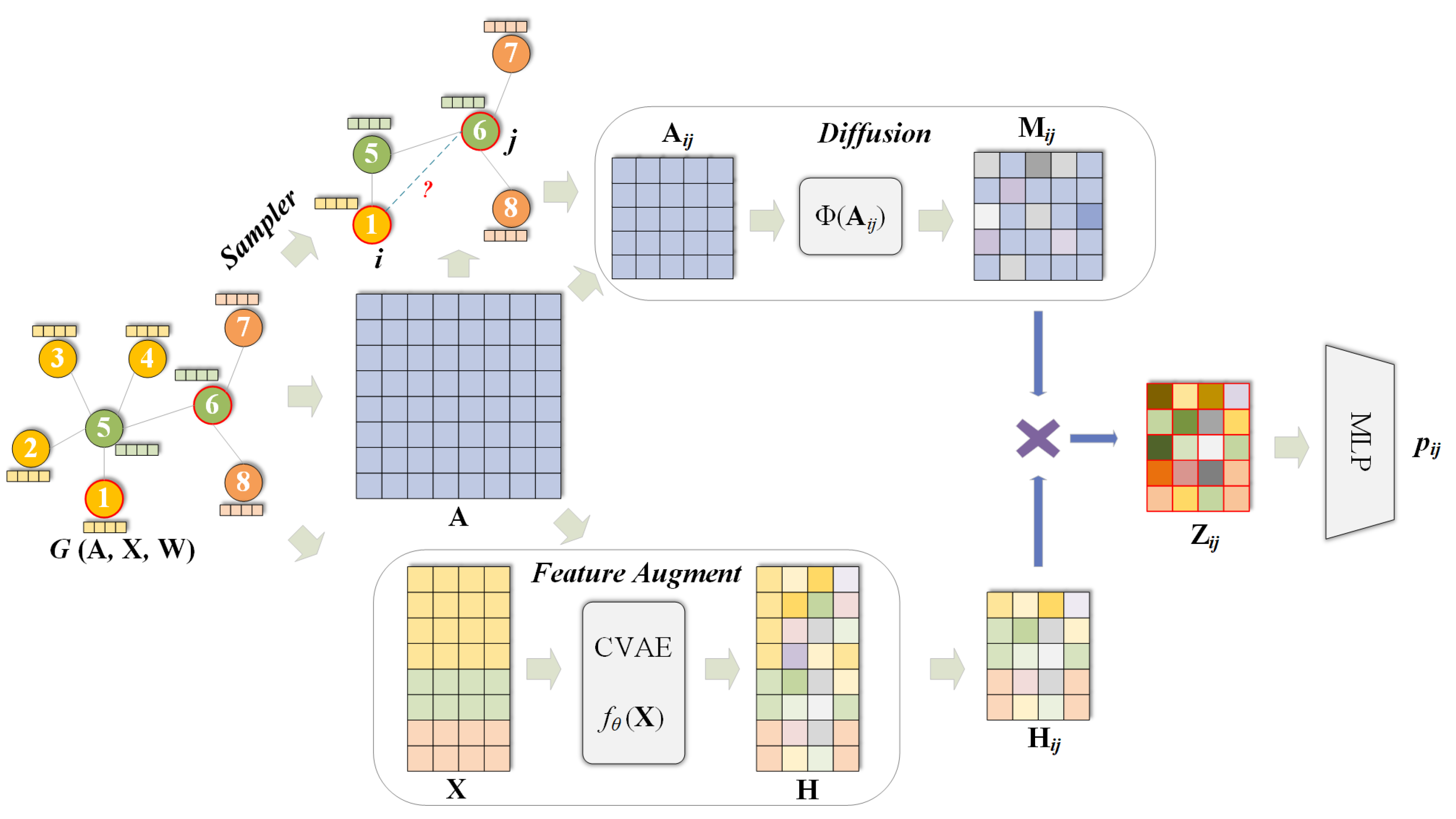
The Augmented Feature Diffusion on Sparsely Sampled Subgraph (AFD3S) process consists of four steps, as Figure 1 illustrates. Firstly, local feature augmentation is applied to the input graph to obtain a feature augmentation matrix. Secondly, sparsely sampled subgraphs are extracted using a random walk strategy, starting from the target node pair. Then, a special weighting operation is performed on the subgraphs, which involves applying a predefined graph diffusion operator to these subgraphs to obtain the diffusion matrix. Finally, the diffusion matrix performs feature diffusion with the previously obtained feature augmentation matrix, resulting in an operator-level node representation of the subgraph. This representation serves as input for downstream link prediction tasks.

3.2. Local Feature Augmentation

Existing GNNs [42] mainly focus on designing message-passing schemes to utilize local information in graphs to obtain node representations. Although GNNs have achieved remarkable performance in various graph-based tasks [8,10,13,14,15,16,17,18,19,20], for the limited local neighborhood information of node numbers, existing GNNs may not fully aggregate such information, thus affecting the learning effect of the models. To address this issue, we propose a local augmentation strategy on graphs, which generates feature distributions of neighbor nodes conditioned on the features of central nodes and utilizes these generated features during the training process to enhance the expressive power of downstream GNNs.

To generate more features within the neighborhood

N_{ν}

of a node v, it is first necessary to know the feature distribution of its neighbor nodes. Since this distribution is related to the central node v, a generative model is used to learn its distribution conditional on the features of the central node. In this paper, we use a Conditional Variational Autoencoder (CVAE) [48] to learn the conditional distribution of the features of the connected neighbor node u (

u \in N_{ν}

) given the central node v. Since the feature distribution of neighbor node u is related to

X_{ν}

, we condition it on

X_{ν}

. The latent variable z is generated from a prior distribution

p_{θ} (z | X_{ν})

, and the generated feature

X_{u}

is produced through a generative distribution conditioned on both z and

X_{ν}

p_{θ} (X ∣ X_{ν}, z)

, i.e.,

z \sim p_{θ} (z | X_{ν})

X_{u} \sim p_{θ} (X ∣ X_{ν}, z_{ν})

. Using

ϕ

to represent variational parameters and

θ

to represent generative parameters, we have:

\begin{matrix} log p_{θ} (X_{u} ∣ X_{ν}) = \int q_{ϕ} (z ∣ X_{u}, X_{ν}) log \frac{p_{θ} (X_{u}, z ∣ X_{ν})}{q_{ϕ} (z ∣ X_{u}, X_{ν})} dz \\ + K L (q_{ϕ} (z ∣ X_{u}, X_{ν}) ∥ p_{θ} (z ∣ X_{u}, X_{ν})) \\ \geq \int q_{ϕ} (z ∣ X_{u}, X_{ν}) log \frac{p_{θ} (X_{u}, z ∣ X_{ν})}{q_{ϕ} (z ∣ X_{u}, X_{ν})} dz \end{matrix}

(1)

the corresponding Evidence Lower Bound (ELBO) [49] can be defined as:

\begin{matrix} L (X_{u}, X_{ν}; θ, ϕ) = - K L (q_{ϕ} (z | X_{u}, X_{ν}) ∥ p_{θ} (z | X_{ν})) + \frac{1}{L} \sum_{l = 1}^{L} \log_{2} p_{θ} (X_{u} | X_{ν}, z^{(l)}) \end{matrix}

(2)

where

z^{(l)} = g_{ϕ} (X_{_{v}}, X_{_{u}}, ϵ^{(l)})

ϵ^{(l)} \sim N (0, I)

, L represents the number of neighbors of node v,

K L

refers to the Kullback-Leibler Divergence [50], also known as relative entropy. In information theory and machine learning,

K L

divergence measures the difference between two probability distributions. In this paper, it is used to measure the difference between the posterior distribution and the prior distribution.

Algorithm 1 CVAE model training

Input:: Input graph G, adjacency matrix $A$ , feature matrix $X$
Output:: Feature generation model $Q_{ϕ}$
1:: Initialize $Q_{ϕ}$
2:: while not convergence do
3:: for each $v \in V$ do
4:: $N_{ν} = g e t_n e i g h b o r s (A, ν)$
5:: $z = e n c o d e r (X_{ν}, Q_{ϕ})$
6:: $X_{_{u}} = g e n e r a t o r (z, X_{_{v}}, N_{_{v}}, Q_{_{ϕ}})$
7:: $l o s s = c o m p u t e_ELBO (X_{ω}, X_{ν}, z, Q_{ϕ})$
8:: $l o s s . b a c k w a r d ()$
9:: $o p t i m i z e r . s t e p ()$
10:: end for
11:: end while
12:: return $Q_{ϕ}$

A CVAE model is trained for all nodes during the experiments. The objective during the training phase is to maximize the ELBO, i.e., Equation (2), by taking pairs of adjacent nodes (

X_{ν}, X_{u}, u \in N_{ν}

) as input. In the Variational Autoencoders (VAE) context, ELBO is typically considered a loss function. During the training of a VAE, the objective is to maximize the ELBO, which is the opposite of minimizing a loss function. Maximizing the ELBO is equivalent to minimizing the sum of the reconstruction error and the

K L

divergence, which helps the model learn latent representations that can generate the data while preserving the structural information in the latent space. During the generation phase, node features

X_{ν}

are used as conditions, and a latent variable

z \sim N (0, I)

is sampled as input to the decoder. Then, a generated feature vector

{\bar{X}}_{ν}

associated with node v can be obtained. Algorithm 1 describes the training process of the CVAE feature generation model.

After training, the generative model is applied to the input graph, and the generated features

{\bar{X}}_{ν}

are used as additional input to perform calculations with the original features

X

to obtain augmented feature representations

H

for the nodes, thus improving the expressive power of downstream GNNs, as shown in Equation (3).

\begin{matrix} H = σ (X, \bar{X}) \end{matrix}

(3)

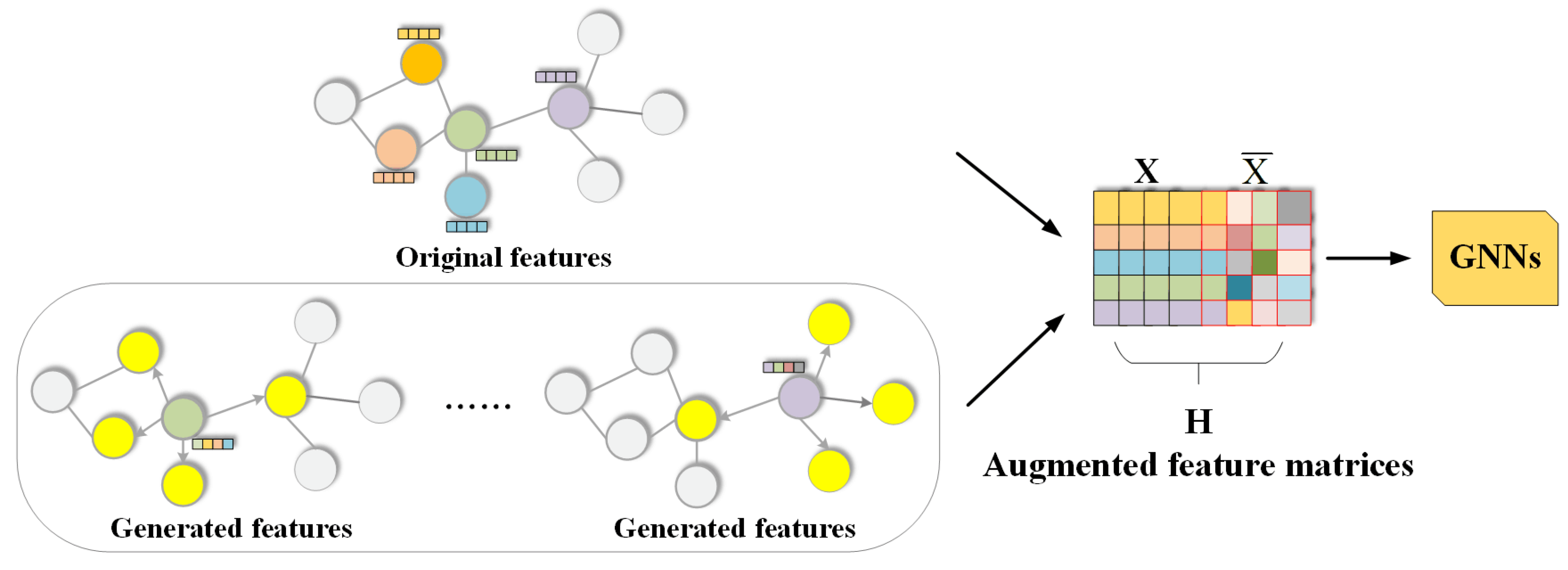
where

σ

represents a specific operation. We provide two ways of using the generated features: concatenation and averaging. Figure 2 illustrates the local feature augmentation using concatenation.

3.3. Subgraph Sampling and Graph Diffusion

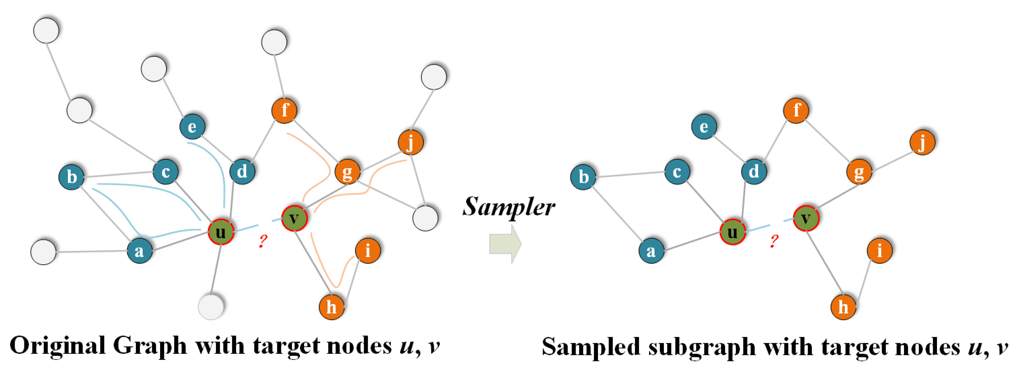
Since SEAL [44] and its variants (WESLP [51], WalkPool [52], etc.) lack scalability, the size of subgraphs grows exponentially as the hop h increases. Nodes with high degrees tend to have very large enclosing subgraphs, even for small hops, resulting in the models’ high temporal and spatial complexity. Therefore, the proposed model utilizes sparsely sampled subgraphs (Definition 2) instead of enclosing subgraphs when extracting subgraphs for a target node pair. By introducing sparsely sampled subgraphs, the model can effectively reduce the size of subgraphs while maintaining sufficient information, thus lowering the temporal and spatial complexity of the model. Figure 3 illustrates the extraction of a sampled subgraph for the target node pair

(u, v)

S_{u}^{h, k} = {a, b, c, d, e}

S_{ν}^{h, k} = {f, g, h, i, j}

V_{u ν}^{h, k} = {a, b, c, d, e, f, g, h, i, j, u, v}

, where the walk length h is 2, and the number of walks k is 3.

By comparing the definitions of enclosing subgraph (Definition 1) and sparsely sampled subgraph, we can draw the following important conclusions: (i) The sampled subgraph

G_{u ν}^{h, k}

is a subgraph of enclosing subgraph

G_{u ν}^{h}

, because random walks of length h cannot reach nodes that are more than h steps away from the starting node; (ii) The size of the sampled subgraph is limited to

O (h k)

, which can be linearly controlled by adjusting the parameters of walk length h and several walks k, in contrast to the exponential growth of enclosing subgraph in Definition 1. By replacing dense enclosing subgraphs with their corresponding sparsely sampled subgraphs, AFD3S reduces the computational and storage overhead of subgraphs, providing scalability while still maintaining the flexibility to control the degree of sparsity and scalability through its sampling parameters h and k.

To obtain the sparsely sampled subgraph

G_{u ν}^{h, k}

for the target node pair

T = {u, v}

, with the corresponding adjacency matrix

A_{u ν}

, to further capture the structural relationships and similarities between nodes, while simulating the process of information diffusion between nodes, the AFD3S utilizes predefined graph diffusion operators to perform specific weighted operations on the sampled subgraph and obtain the corresponding diffusion matrix:

\begin{matrix} M_{u ν} = ψ (A_{u ν}) \end{matrix}

(4)

where,

M_{u ν}

represents the diffusion matrix of the sampled subgraph, and

G_{u ν}^{h, k}

denotes the specific graph diffusion operator.

ψ

can be varied by using different diffusion operators to capture different structural features in the graph, such as adjacency matrices/Laplacian operators for capturing connectivity, triangle/motif-based operators [53] for capturing inherent community structures, and Personalized PageRank (PPR)-based operators [54] for identifying important connections. Each operator and its powers can constitute different diffusion operators in AFD3S. The graph diffusion operator used in this model is the multiple powers of the adjacency matrix, which captures and represents the multi-hop neighborhood relationships of nodes in the graph, providing rich topological features for graph structure analysis and GNNs.

3.4. Feature Diffusion

The diffusion matrix

M_{u v}

of the sampled subgraph is used to perform feature diffusion operations with the corresponding feature augmentation matrix

H_{u v}

, obtaining the operator-level node representation

Z_{u v}

of the subgraph:

\begin{matrix} Z_{u ν} = M_{u ν} \cdot H_{u ν} \end{matrix}

(5)

Feature diffusion simulates the process of information diffusion between nodes, simplifying subgraph representation learning. The operator-level node feature representation not only contains its information but also integrates information from its neighbor nodes, thus capturing the structural characteristics within the subgraph. Specifically, feature diffusion operations help with:

Feature smoothing: In deep GNNs, information may propagate excessively between nodes, leading to overly similar node representations and the issue of over-smoothing. Adjusting the diffusion matrix can somewhat alleviate this problem, maintaining the diversity of node representations.
Enhancing node representations: A node’s feature vector can integrate features from its direct and indirect neighbors through diffusion operations, making the node representation richer and more comprehensive.
Simulating graph structure: The diffusion matrix essentially reflects the structural information of the graph. Multiplying it with the feature augmentation matrix can simulate information transmission between nodes based on the graph structure, simplifying the subgraph representation learning process and accelerating training and inference speeds.
Improving prediction performance: In link prediction tasks, this node representation fused with structural information can improve the model’s accuracy in predicting potential links, as it can better capture the interdependencies between nodes.
Computational efficiency: Compared to performing complex graph neural network operations on the entire graph, this subgraph-level diffusion operation can significantly reduce the amount of computation, making the model more efficient for applications on large-scale graphs.

In experiments, one can apply a set of different graph diffusion operators to the same sampled subgraph to obtain a set of linear diffusion matrices

M_{u ν}^{(0)}, . . ., M_{u ν}^{(r)}

. These diffusion matrices are then applied to the feature augmentation matrix

H_{u ν}

of the subgraph to yield a set of operator-level node representations

Z_{u ν}^{(0)}, . . ., Z_{u ν}^{(r)}

. Furthermore, it holds that:

\begin{matrix} Z_{u ν}^{(i)} = M_{u ν}^{(i)} \cdot H_{u ν} \end{matrix}

(6)

where

M_{u ν}^{(i)}

represents the diffusion matrix corresponding to the adjacency matrix of the subgraph when the i-th diffusion operator is applied. Then, the operator-level node representation matrices

Z_{u ν}^{(i)}

of all sampled subgraphs are concatenated to form the final joint node representation, which is given by

\begin{matrix} Z_{u ν} = ⨁_{i = 0}^{r} Z_{u ν}^{(i)} \end{matrix}

(7)

where the ⨁ symbol represents the concatenation operation of a set of feature vectors. When concatenating node representation matrices with mismatched dimensions, it is necessary to ensure that the rows belonging to the same node are properly aligned. For any missing rows, zero-padding is used, similar to the zero-padding strategy in graph pooling, thus ensuring the uniformity of matrix dimensions and data integrity.

3.5. Training and Prediction

After obtaining the final operator-level node feature matrix

Z_{u ν}

of the sampled subgraph, the first step is to reduce the dimensionality of the node representation matrix. This can be achieved through a fully connected layer consisting of a learnable weight matrix

W

and a nonlinear activation function

δ

. The purpose of this step is to reduce the dimensionality of the node representation while preserving important information. Next, a pooling operation is performed on the reduced representation. This typically involves aggregating the representations of the target node and its common neighbors. Pooling methods can be center pooling or center-common-neighbor pooling, which help further extract and integrate critical information. Finally, the pooled representation is input into a learnable function

ζ

, such as a Multi-Layer Perceptron(MLP), which transforms the node representation into the probability

p_{u ν}

of a link existing. This probability can then be used for link prediction tasks. The above process is formulated as follows:

\begin{matrix} p_{u ν} = ζ (p o o l (δ (Z_{u ν} W))) \end{matrix}

(8)

During the training process, the model optimizes the weight matrix

W

and the parameters of function

ζ

by minimizing the difference between the predicted link probability and the actual existence of the link. This is typically achieved through optimization techniques such as backpropagation and gradient descent. The training loss function employs the binary cross-entropy loss function, whose formula is as follows:

\begin{matrix} L = - \frac{1}{|E_{l a b e l}|} \sum_{(u, ν) \in E_{l a b e l}} [y_{u ν} log p_{u ν} + (1 - y_{u ν}) log (1 - p_{u ν})] \end{matrix}

(9)

where

E_{l a b e l}

represents the entire training set,

|E_{l a b e l}|

represents the number of samples,

y_{u ν}

indicates whether there exists an edge between nodes u and v, and

p_{u ν}

represents the predicted probability of the existence of an edge. This loss function minimizes the cross-entropy between the predicted results and the true labels. Algorithm 2 describes the process of AFD3S for link prediction training.

Algorithm 2 Augmented Feature Diffusion on Sparsely Sampled Subgraph (AFD3S)

Input:: Input graph G, adjacency matrix $A$ , feature matrix $X$
Output:: Link prediction model $Ω$
1:: Initialize $Ω, W, δ$
2:: $H = l o c a l_a u g m e n t (A, X, σ)$
3:: while not convergence do
4:: for each $(u, v) \in E$ do
5:: $G_{u v}^{h, k}, A_{u v} = S a m p l e r (A, h, k, u, v)$
6:: for $i = 1 \to r$ do
7:: $M_{u v}^{(i)} = ψ^{(i)} (A_{u v})$
8:: $Z_{u v}^{(i)} = M_{u v}^{(i)} \cdot H_{u v}$
9:: end for
10:: $Z_{u v} = a g g r e g a t e_Z (Z_{u v}^{(0)}, . . ., Z_{u v}^{(r)})$
11:: $p_{u v} = ζ (p o o l (δ (Z_{u v} W)))$
12:: $l o s s = c o m p u t e_l o s s (Ω, p_{w}, y_{w})$
13:: $l o s s . b a c k w a r d ()$
14:: $o p t i m i z e r . s t e p ()$
15:: end for
16:: end while
17:: return $Ω$

4. Experiment

4.1. Datasets and Baselines

Datasets: We used nine real-world network datasets, including weighted and unweighted, undirected, attributed, and non-attributed graph data. The experiments divided these datasets into two categories: non-attributed and attributed datasets. For both attributed and non-attributed datasets, except for Cora, CiteSeer, and PubMed, which were divided into 70% training set, 10% validation set, and 20% test set according to specific experimental settings, the edges of the remaining datasets were randomly divided into 85% training set, 5% validation set, and 10% test set. The experimental datasets include NS [55], a collaboration network of network science researchers, Power [43], an electrical power grid of the western United States, Yeast [56], a protein-protein interaction network, PB [57], a political blog network, Cora [58], a citation network in the field of machine learning, CiteSeer [59], a scientific publication citation network, PubMed [59], a diabetes-related scientific publication citation network, and Texas and Wisconsin [60], web page datasets collected by computer science departments of different universities.

Table 1 details the statistical information of these datasets, with the first four being non-attributed networks and the last five being attributed networks. Node represents the number of nodes, Edge represents the number of edges, Avg Deg represents the average degree of the network, Feat represents the feature dimension of the nodes, and Type represents the network type.

Baselines: In this section, we experimentally analyze the proposed link prediction model AFD3S and compare it with nine existing advanced link prediction models on nine different real-world datasets. These include two message-passing graph neural network (MPGNNs) models: GCN [61] and GIN [62]; three autoencoder (AE) models: GAE, VGAE [63], and GIC (Graph InfoClust) [64]; and four SGRLs: SEAL [44], WESLP [51], Scaled [45], and WalkPool [52].

4.2. Experimental Setup

Experimental Environment: Equipped with AMD Ryzen 7 5800H CPU, 32GB memory The hardware environment of NVIDIA GeForce RTX 3070 Laptop GPU (8GB graphics memory) runs on the Windows 11 64-bit operating system, using PyCharm 2023.2.1 as the development tool, Python 3.10.9 as the development language, and PyTorch 1.12.1 and PyTorch Geometry 2.0.9 as the development framework.

Experimental Settings: For SGRLs and the AFD3S method on non-attributed datasets, the hop of the enclosing subgraphs, h, is typically set to 2 (except for the WalkPool on the Power dataset, where h is set to 3). For sparsely sampled subgraphs, the walk length h is set to 2, and the number of walks k is set to 50. On attributed datasets, the hop of the enclosing subgraphs, h, is generally set to 3 (while the WalkPool sets it to 2). The settings for sparsely sampled subgraphs are the same as for non-attributed datasets. Additionally, in the AFD3S, the zero-one [38] labeling scheme is uniformly adopted to label all datasets, while models like SEAL and Scaled use DRNL [44] for labeling. The central common neighbor pooling readout function employs a simple mean aggregation approach. These settings and choices aim to ensure consistency and performance optimization of the models while accommodating the characteristics of different datasets and models. Moreover, for all datasets, the percentages of training, validation, and test sets across all models are uniformly set to 85%, 5%, and 10%, respectively, with a 1:1 sampling ratio for positive and negative samples.

In the AFD3S model, the neural network utilizes SIGN [65], and for the non-attributed datasets, Node2Vec is employed to generate 256-dimensional feature vectors for each node. In the process of feature augmentation,

σ

uniformly adopts concatenation as the augmentation method. For all datasets, the hidden dimension after pooling in Equation (8) is set to 256, and an MLP with a 256-dimensional hidden layer is adopted in the experiments. To maintain consistency, the dropout rate is set to 0.5 for all models, the learning rate is set to 0.0001, and the Adam optimizer is used for 50 training epochs. During the training process, except for the MPGNN model, which uses full-batch training on the input graph, the batch size for other models is set to 32. These settings ensure the experiments’ fairness and comparability while fully utilizing the potential of the AFD3S model.

Evaluation Metrics: This paper adopts AUC and AP as the evaluation standards for model performance, aiming to accurately assess the performance of the AFD3S in solving the link prediction problem. Additionally, to fully demonstrate the computational efficiency and scalability of the AFD3S, this study further compares the performance of the AFD3S with existing popular SGRLs in terms of average preprocessing time, average training time, average inference time, and total running time.

4.3. Results and Analysis

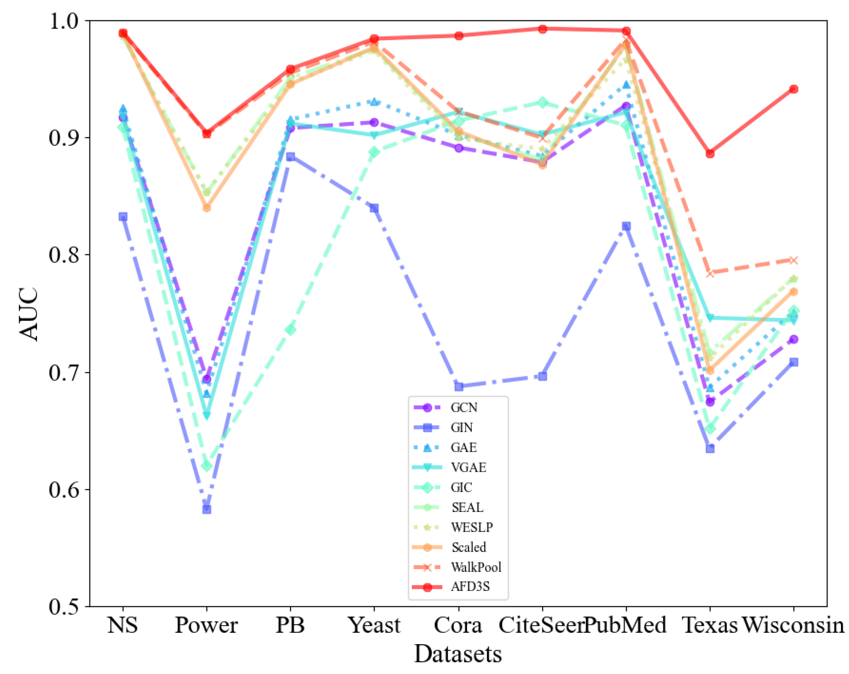
Link Prediction: For all models, on both attributed and non-attributed datasets, this study presents the average AUC and AP scores over 10 runs with different fixed random seeds on the test data. Table 2 displays the AUC results for both non-attribute and attribute datasets, while Table 3 displays the AP results for both non-attribute and attribute datasets. The optimal values are marked in bold.

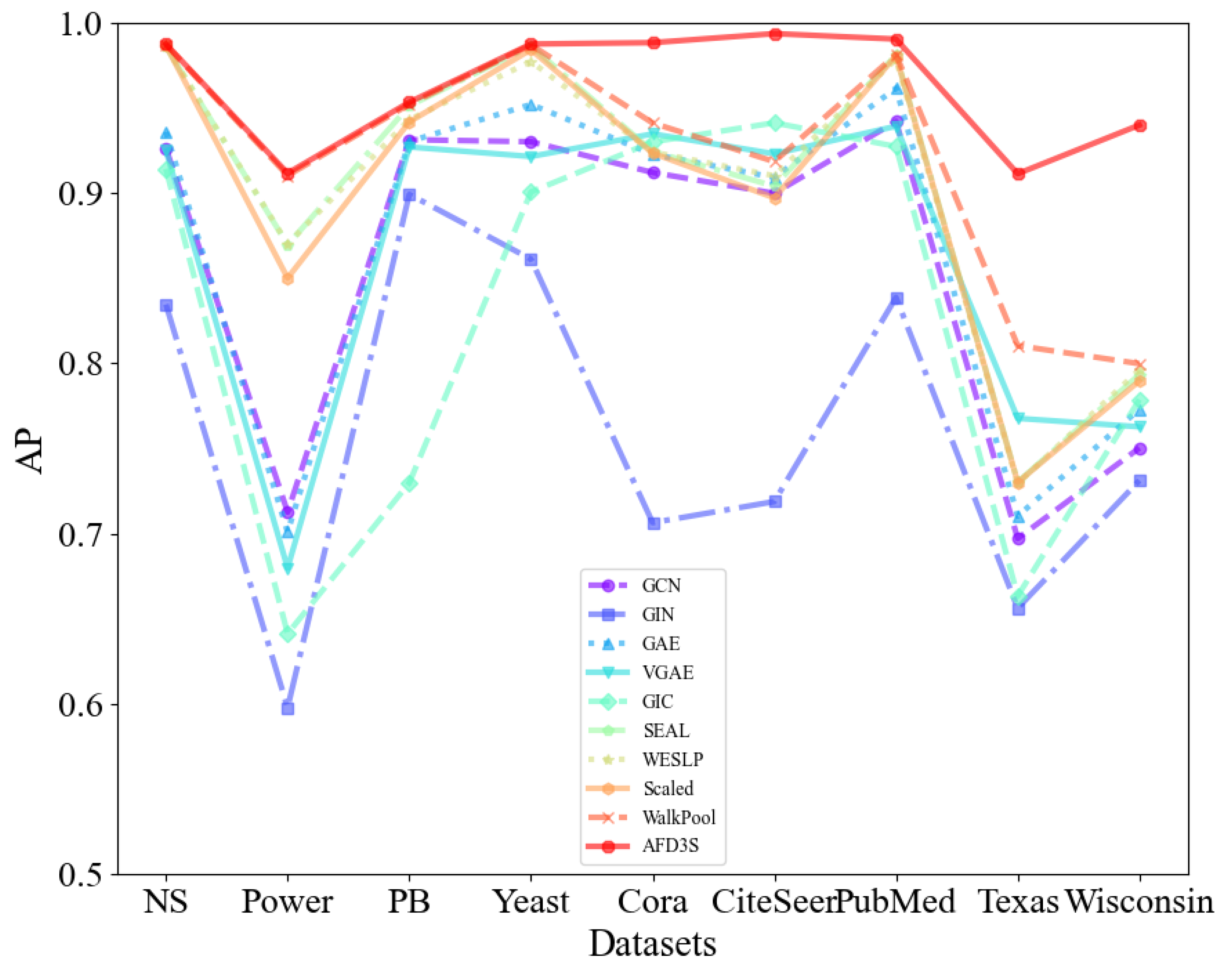
Based on the data in Table 2 and Table 3, it is evident that the proposed AFD3S demonstrates exceptional performance in terms of average AUC and AP results on both non-attributed and attributed datasets, achieving optimal levels. Specifically, on attributed datasets, compared to the advanced benchmark model WalkPool, the AUC results of the AFD3S show improvements of 6.44% on Cora, 9.32% on CiteSeer, 10.23% on Texas, and 14.57% on Wisconsin. Simultaneously, the AUC and AP results of the AFD3S on non-attributed datasets also exhibit a certain degree of improvement.

Figure 4. The average AUC of all models on attributed and non-attributed datasets (over 10 runs).

Figure 5. The average AP of all models on attributed and non-attributed datasets (over 10 runs).

The significant advantage is the importance of node features in node classification and graph classification tasks. The node features of attributed datasets provide direct, rich, and semantically clear information whose expressive power is often superior to node features generated based on random walks. This direct utilization of original node features helps improve the interpretability and stability of the model while reducing additional computational costs. Furthermore, the AFD3S incorporates the neighboring node features of the central node during the local feature augmentation process, enabling it to capture complex relationships between nodes. This approach fully utilizes the multi-source information of graph data, providing superior performance for downstream tasks of GNNs. Therefore, the superior performance of the AFD3S on various datasets demonstrates its effectiveness and practicability in link prediction tasks.

Computational Efficiency: To further validate the computational efficiency and scalability of the AFD3S, this paper selects three currently popular and performance-advanced SGRLs—SEAL, GCN+DE (distance encoding) [60], and WalkPool, and conducts comparative experiments on all datasets. The comparative experiments mainly focus on four key indicators: preprocessing time, average training time (50 epochs), average inference time, and total runtime (50 epochs), aiming to comprehensively demonstrate the computational efficiency of the AFD3S in practical applications. Table 4 and Table 5 present the experimental results on non-attributed and attributed datasets. In these tables, “Train” represents the average training time for 50 epochs, “Inference” represents the average inference time, “Preproc.” represents the preprocessing time, and “Runtime” represents the average runtime for 50 epochs. The fastest values are bolded, and the maximum (minimum) speedup ratio in “Speed up” refers to the ratio of the time required by the slowest (fastest) SGRL methods to the AFD3S model.

Through experimental results, we can observe that the AFD3S proposed in this paper has achieved significant acceleration in training, inference, and running time compared with other SGRLs on all datasets. Specifically, the training speed is improved by 3.34 to 17.95 times, the inference speed is accelerated by 3 to 61.05 times, and the overall running time is shortened by 2.27 to 14.53 times. Although the preprocessing time of the AFD3S model is relatively high, due to the significant improvement in training and inference speeds, this difference is effectively offset, making the maximum acceleration reach 14.53 times on the Yeast dataset. It is worth noting that as the scale of the dataset increases, the computational time acceleration effect of the AFD3S becomes particularly evident. The highest acceleration multiples are achieved on the three large PubMed, PB, and Yeast datasets, demonstrating the excellent performance of the AFD3S in computational efficiency and scalability.

This gain is primarily attributed to the innovative strategies employed by the AFD3S. Adopting a random walk-based strategy to sample sparse subgraphs instead of enclosing subgraphs significantly reduces subgraphs’ storage and computational overhead. As the graph size increases, the scale of extracted subgraphs decreases from exponential to linear, reducing computational complexity and improving model efficiency. Additionally, the randomness in random walks brings additional regularization benefits to the model, further enhancing its performance. Meanwhile, the AFD3S utilizes easily pre-computed subgraph-level diffusion operators to replace expensive message-passing schemes through feature diffusion, significantly improving training and inference speeds. These optimization measures collectively enable the AFD3S to demonstrate excellent computational efficiency and scalability in link prediction tasks.

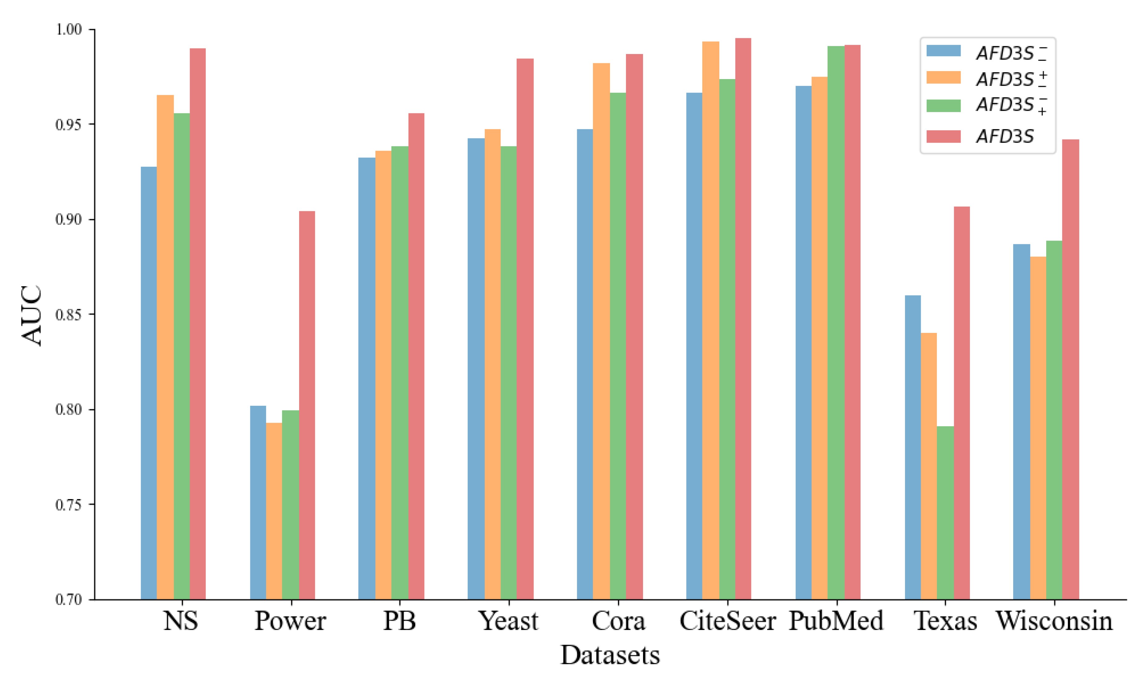
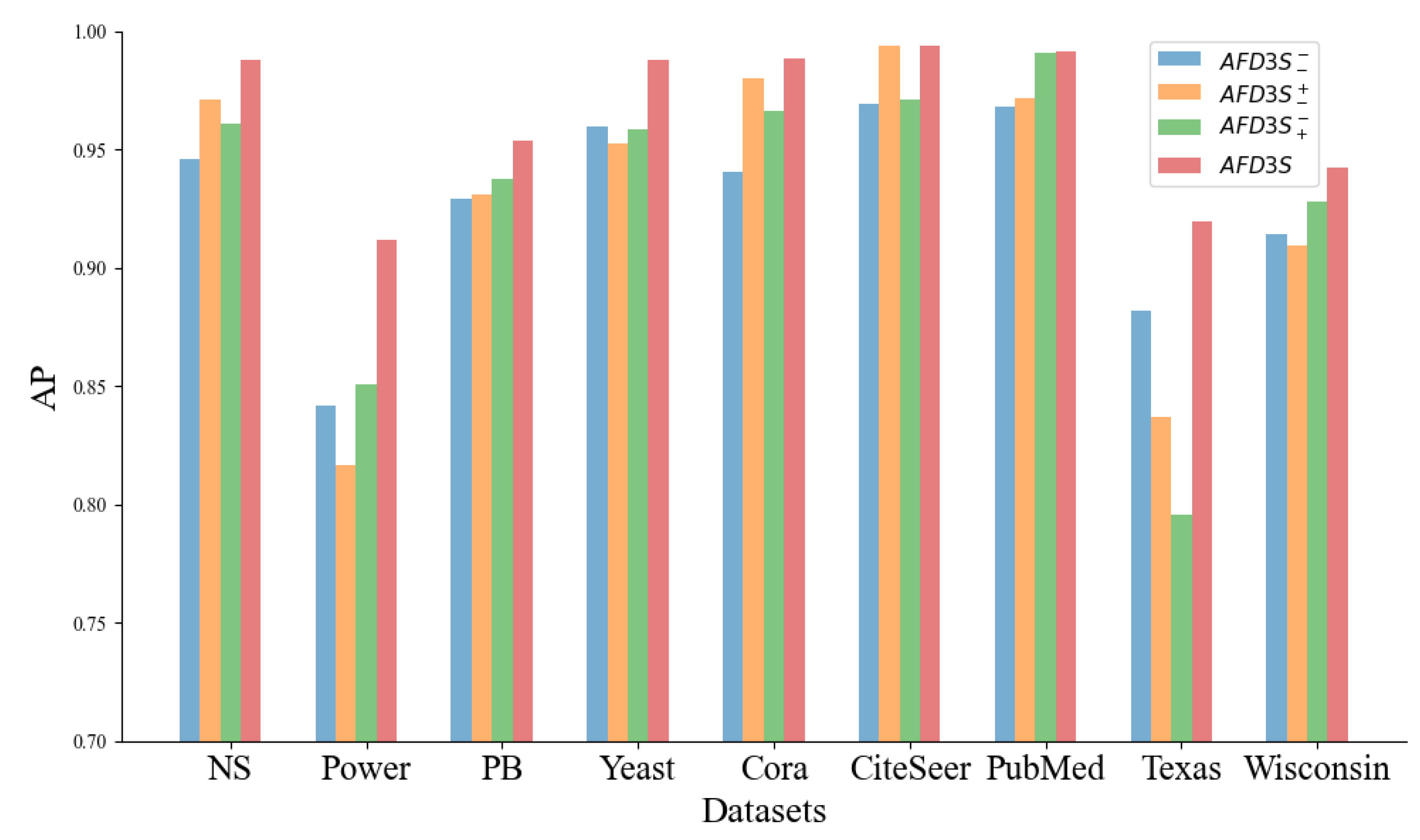
Ablation Study: We conducted an ablation study to further explore the key factors contributing to the performance gains of the AFD3S, specifically verifying the effectiveness of local feature augmentation and graph diffusion operations on the predictive performance of the AFD3S. Three variants of the AFD3S were designed and compared with the original AFD3S in terms of AUC and AP metrics for link prediction across all datasets. The three variants are: 1) Variant

AFD 3 S_{-}^{-}

, which does not perform local feature augmentation and graph diffusion operations; 2) Variant

AFD 3 S_{-}^{+}

, which performs local feature augmentation but does not perform graph diffusion operations; 3) Variant

AFD 3 S_{+}^{-}

, which performs graph diffusion operations but does not perform local feature augmentation. The experimental results are presented in Figure 6 and Figure 7.

Observing the experimental results, it can be seen that on most datasets, among the three variants of AFD3S, the link prediction performance of Variant

AFD 3 S_{-}^{+}

using local augmentation alone and Variant

AFD 3 S_{+}^{-}

using graph diffusion alone both show some degree of improvement compared to Variant

AFD 3 S_{-}^{-}

without any augmentation. This proves the effectiveness of the two augmentation strategies proposed in this paper for AFD3S in link prediction tasks. Furthermore, when local feature augmentation and graph diffusion operations are used simultaneously (i.e., the original AFD3S), the performance is improved on all datasets, with significant improvements on most datasets. The main reason is that after local feature augmentation, the subsequent graph diffusion operation amplifies this augmentation effect, significantly improving subsequent prediction performance.

Specifically, since the AFD3S extracts sparsely sampled subgraphs of target node pairs to reduce subgraphs’ storage and computational efficiency, it cannot, in most cases, include all h-hop neighbor nodes of the target node pairs as enclosing subgraphs can. However, the local feature augmentation operation is based on the original input graph, fusing features from other neighbor nodes of the central node through feature augmentation, thus compensating for the shortcomings of sparse subgraphs. This augmentation is further amplified by the graph diffusion operation, and it can capture the structural relationships and similarities between nodes. At the same time, it simulates the information diffusion process between nodes through feature diffusion to simplify the information transmission and aggregation operations in subgraph representation learning, accelerating the training and inference speed of downstream tasks.

In summary, AFD3S improves the link prediction performance and reduces subgraphs’ storage and computational overhead, enhancing the model’s computational efficiency and scalability. It provides an efficient and practical solution for graph analysis tasks.

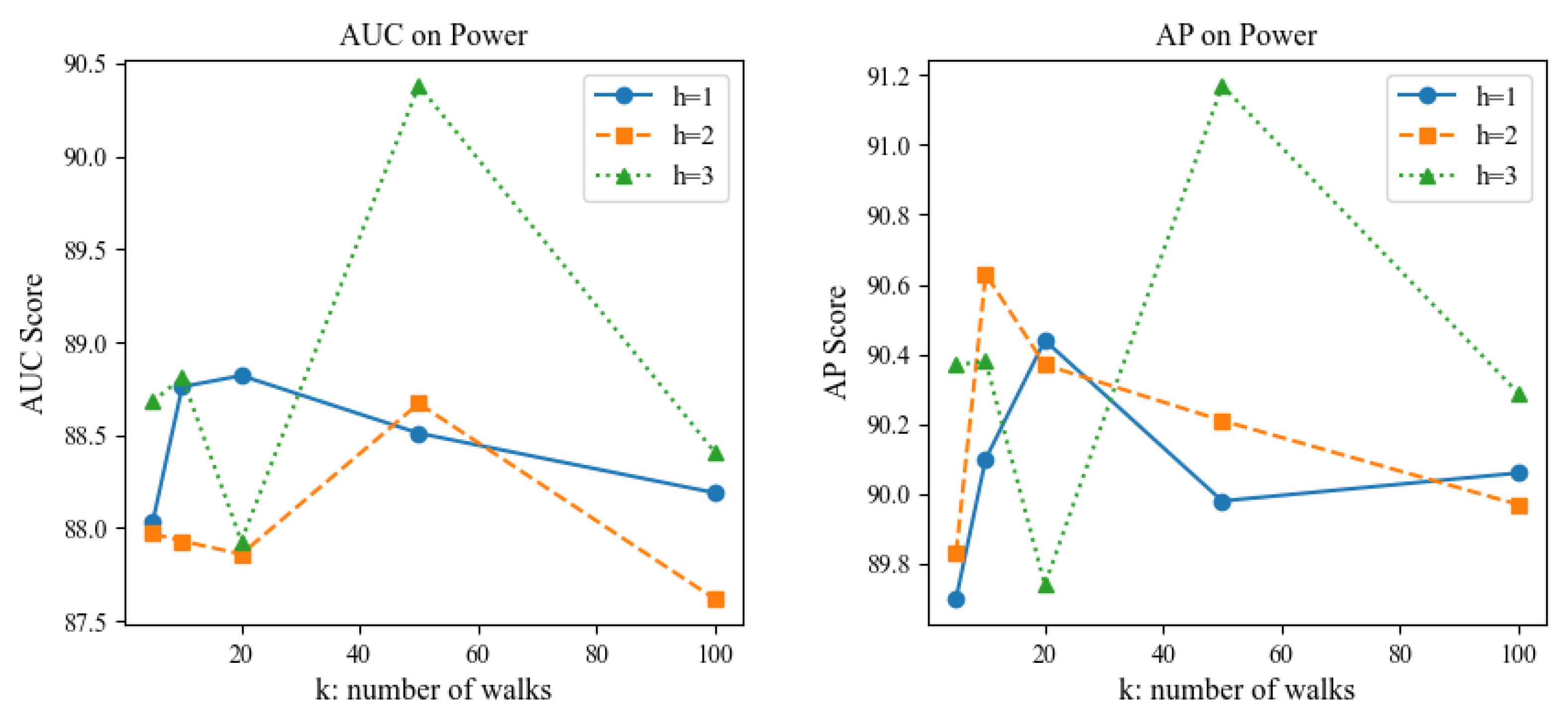
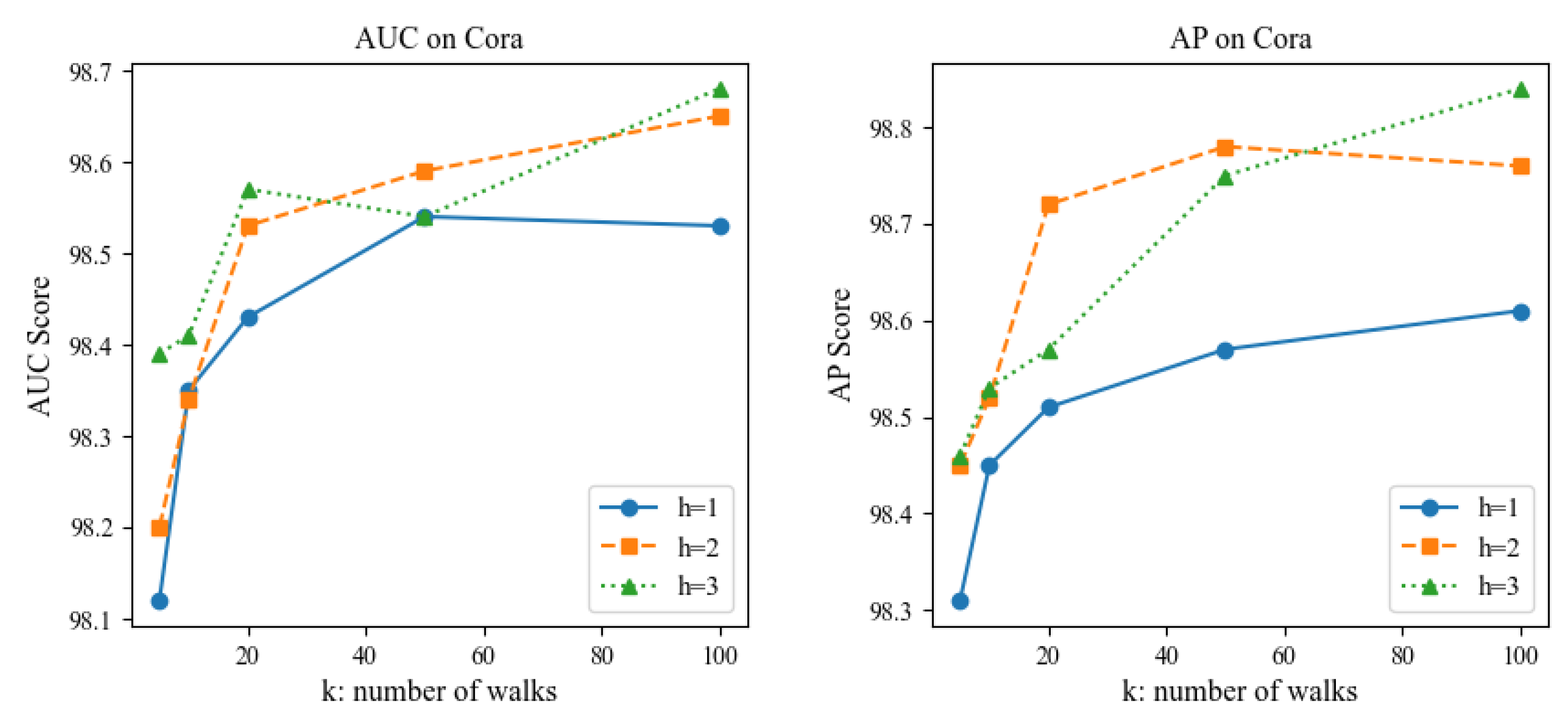
Parameter Sensitivity: We also conducted a sensitivity analysis on the two hyperparameters of the extracted sparsely sampled subgraph, namely the walk length h and the number of walks k, to investigate the impact of the size of the sampled subgraph on the link prediction performance of the AFD3S. Due to certain similarities across different datasets, experiments were performed on the Power non-attribute and Cora attribute datasets as examples. All other parameters remained unchanged in the experiments except for the test variable to maintain fairness. The experimental results are shown in Figure 8 and Figure 9.

The experimental results show that the AFD3S performs excellent prediction even when using smaller h and k values. Notably, when the extracted subgraph is too large, the prediction performance decreases compared to a smaller subgraph. This is likely because a larger subgraph may contain nodes and edges irrelevant to the target link prediction task. Such noise and irrelevant information may interfere with the model’s learning process, leading the model to capture incorrect patterns and thus reducing prediction accuracy. This finding further proves that the AFD3S can extract key information from sparse and small sampled subgraphs, significantly improving computational efficiency while ensuring prediction performance. Additionally, it demonstrates the superiority and scalability of AFD3S in handling large-scale graph data. The AFD3S can more effectively cope with large-scale graph data by reducing computational and storage overhead, providing strong support for practical applications.

5. Conclusions

In this paper, we propose a novel SubGraph Representation Learning (SGRL) framework called Augmented Feature Diffusion on Sparsely Sampled Subgraph (AFD3S). AFD3S integrates neighborhood features for central nodes through local feature augmentation and utilizes a random walk strategy to sample sparse subgraphs, effectively reducing the storage and computational requirements of the subgraphs. Additionally, by introducing subgraph-level diffusion operators that can be easily precomputed, AFD3S employs feature diffusion operations to replace the traditional expensive message-passing schemes, simplifying the subgraph representation learning process and further accelerating the training and inference processes. Finally, experimental results on multiple real-world datasets show that compared to existing SGRLs, the proposed AFD3S significantly improves computational speed and exhibits higher link prediction performance. These results fully demonstrate the excellent performance, computational efficiency, and scalability of the AFD3S for link prediction tasks.

Author Contributions

Conceptualization, methodology, formal analysis, investigation, data curation, visualization, writing—original draft preparation, X.W. and H.C.; supervision, resources, project administration, funding acquisition, writing—review and editing, X.W. and H.C.. All authors have read and agreed to the published version of the manuscript.

Funding

This research received no external funding.

Institutional Review Board Statement

Not applicable.

Informed Consent Statement

Not applicable.

Data Availability Statement

There is no data associated with this manuscript.

Conflicts of Interest

The authors declare no conflicts of interest.

References

Nie, M.; Chen, D.; Wang, D. Reinforcement learning on graphs: A survey. IEEE Transactions on Emerging Topics in Computational Intelligence 2023. [CrossRef]
Adamic, L.A.; Adar, E. Friends and neighbors on the web. Social networks 2003, 25, 211–230. [Google Scholar] [CrossRef]
Chen, L.; Xie, Y.; Zheng, Z.; Zheng, H.; Xie, J. Friend recommendation based on multi-social graph convolutional network. IEEE Access 2020, 8, 43618–43629. [Google Scholar] [CrossRef]
Huang, X.; Chen, D.; Ren, T.; Wang, D. A survey of community detection methods in multilayer networks. Data Mining and Knowledge Discovery 2021, 35, 1–45. [Google Scholar] [CrossRef]
Oyetunde, T.; Zhang, M.; Chen, Y.; Tang, Y.; Lo, C. BoostGAPFILL: improving the fidelity of metabolic network reconstructions through integrated constraint and pattern-based methods. Bioinformatics 2017, 33, 608–611. [Google Scholar] [CrossRef] [PubMed]
Zitnik, M.; Agrawal, M.; Leskovec, J. Modeling polypharmacy side effects with graph convolutional networks. Bioinformatics 2018, 34, i457–i466. [Google Scholar] [CrossRef] [PubMed]
Zhang, W.; Xu, D.; others. Evolving model for the complex traffic and transportation network considering self-growth situation. Discrete Dynamics in Nature and Society 2012, 2012.
Wang, L. Analysis and Evaluation of Kinect-based Action Recognition Algorithms. Master’s thesis, School of the Computer Science and Software Engineering, The University of Western Australia, 2017. [CrossRef]
Wang, L.; Huynh, D.Q.; Mansour, M.R. Loss switching fusion with similarity search for video classification. 2019 IEEE international conference on image processing (ICIP). IEEE, 2019, pp. 974–978.
Wang, L.; Huynh, D.Q.; Koniusz, P. A comparative review of recent kinect-based action recognition algorithms. IEEE Transactions on Image Processing 2019, 29, 15–28.
Wang, L.; Koniusz, P.; Huynh, D.Q. Hallucinating idt descriptors and i3d optical flow features for action recognition with cnns. Proceedings of the IEEE/CVF international conference on computer vision, 2019, pp. 8698–8708.
Wang, L.; Koniusz, P. Self-supervising action recognition by statistical moment and subspace descriptors. Proceedings of the 29th ACM international conference on multimedia, 2021, pp. 4324–4333.
Koniusz, P.; Wang, L.; Cherian, A. Tensor representations for action recognition. IEEE Transactions on Pattern Analysis and Machine Intelligence 2021, 44, 648–665. [Google Scholar] [CrossRef] [PubMed]
Qin, Z.; Liu, Y.; Ji, P.; Kim, D.; Wang, L.; Anwar, S.; Gedeon, T. Fusing higher-order features in graph neural networks for skeleton-based action recognition. IEEE Transactions on Neural Networks and Learning Systems 2022, 35, 4783–4797. [Google Scholar] [CrossRef] [PubMed]
Wang, L.; Koniusz, P. Uncertainty-dtw for time series and sequences. European Conference on Computer Vision. Springer, 2022, pp. 176–195.
Wang, L.; Koniusz, P. 3mformer: Multi-order multi-mode transformer for skeletal action recognition. Proceedings of the IEEE/CVF Conference on Computer Vision and Pattern Recognition, 2023, pp. 5620–5631.
Wang, L.; Koniusz, P. Temporal-viewpoint transportation plan for skeletal few-shot action recognition. Proceedings of the Asian Conference on Computer Vision, 2022, pp. 4176–4193.
Wang, L.; Liu, J.; Koniusz, P. 3D Skeleton-based Few-shot Action Recognition with JEANIE is not so Naïve. arXiv preprint arXiv:2112.12668, 2021. [Google Scholar] [CrossRef]
Wang, L.; Liu, J.; Zheng, L.; Gedeon, T.; Koniusz, P. Meet JEANIE: a Similarity Measure for 3D Skeleton Sequences via Temporal-Viewpoint Alignment. International Journal of Computer Vision, 2024; 1–32. [Google Scholar]
Wang, L. Robust human action modelling. PhD thesis, The Australian National University (Australia), 2023.
Wang, L.; Koniusz, P. Flow dynamics correction for action recognition. ICASSP 2024-2024 IEEE International Conference on Acoustics, Speech and Signal Processing (ICASSP). IEEE, 2024, pp. 3795–3799.
Wang, L.; Sun, K.; Koniusz, P. High-order tensor pooling with attention for action recognition. ICASSP 2024-2024 IEEE International Conference on Acoustics, Speech and Signal Processing (ICASSP). IEEE, 2024, pp. 3885–3889.
Chen, W.; Xiao, H.; Zhang, E.; Hu, L.; Wang, L.; Liu, M.; Chen, C. SATO: Stable Text-to-Motion Framework. ACM-MM, 2024. [Google Scholar]
Fang, S.; Wang, L.; Zheng, C.; Tian, Y.; Chen, C. SignLLM: Sign Languages Production Large Language Models. arXiv preprint arXiv:2405.10718, 2024. [Google Scholar]
Chen, Q.; Wang, L.; Koniusz, P.; Gedeon, T. Motion meets Attention: Video Motion Prompts. arXiv preprint arXiv:2407.03179, arXiv:2407.03179 2024.
Wang, L.; Yuan, X.; Gedeon, T.; Zheng, L. Taylor videos for action recognition. ICML 2024. [Google Scholar]
Zhu, L.; Wang, L.; Raj, A.; Gedeon, T.; Chen, C. Advancing Video Anomaly Detection: A Concise Review and a New Dataset. arXiv preprint arXiv:2402.04857, 2024. [Google Scholar]
Lü, L.; Medo, M.; Yeung, C.H.; Zhang, Y.C.; Zhang, Z.K.; Zhou, T. Recommender systems. Physics reports 2012, 519, 1–49. [Google Scholar] [CrossRef]
Newman, M.E. Clustering and preferential attachment in growing networks. Physical review E 2001, 64, 025102. [Google Scholar] [CrossRef] [PubMed]
Katz, L. A new status index derived from sociometric analysis. Psychometrika 1953, 18, 39–43. [Google Scholar] [CrossRef]
Chen, D.; Nie, M.; Xie, F.; Wang, D.; Chen, H. Link Prediction and Graph Structure Estimation for Community Detection. Mathematics 2024, 12, 1269. [Google Scholar] [CrossRef]
Hamilton, W.L. Graph representation learning; Morgan & Claypool Publishers, 2020.
Nie, M.; Chen, D.; Wang, D. Graph embedding method based on biased walking for link prediction. Mathematics 2022, 10, 3778. [Google Scholar] [CrossRef]
Wu, Z.; Pan, S.; Chen, F.; Long, G.; Zhang, C.; Philip, S.Y. A comprehensive survey on graph neural networks. IEEE transactions on neural networks and learning systems 2020, 32, 4–24. [Google Scholar] [CrossRef]
Zhou, J.; Cui, G.; Hu, S.; Zhang, Z.; Yang, C.; Liu, Z.; Wang, L.; Li, C.; Sun, M. Graph neural networks: A review of methods and applications. AI open 2020, 1, 57–81. [Google Scholar] [CrossRef]
Dai, H.; Dai, B.; Song, L. Discriminative embeddings of latent variable models for structured data. International conference on machine learning. PMLR, 2016, pp. 2702–2711.
Li, Y.; Tarlow, D.; Brockschmidt, M.; Zemel, R. Gated graph sequence neural networks. arXiv preprint arXiv:1511.05493, arXiv:1511.05493 2015.
Zhang, M.; Li, P.; Xia, Y.; Wang, K.; Jin, L. Labeling trick: A theory of using graph neural networks for multi-node representation learning. Advances in Neural Information Processing Systems 2021, 34, 9061–9073. [Google Scholar]
Cai, L.; Li, J.; Wang, J.; Ji, S. Line graph neural networks for link prediction. IEEE Transactions on Pattern Analysis and Machine Intelligence 2021, 44, 5103–5113. [Google Scholar] [CrossRef] [PubMed]
Chen, H.; Chen, J.; Liu, D.; Zhang, S.; Hu, S.; Cheng, Y.; Wu, X. Link Prediction Based on the Sub-graphs Learning with Fused Features. International Conference on Neural Information Processing. Springer, 2023, pp. 253–264.
Li, W.; Gao, Y.; Li, A.; Zhang, X.; Gu, J.; Liu, J. Sparse Subgraph Prediction Based on Adaptive Attention. Applied Sciences 2023, 13, 8166. [Google Scholar] [CrossRef]
Scarselli, F.; Gori, M.; Tsoi, A.C.; Hagenbuchner, M.; Monfardini, G. The graph neural network model. IEEE transactions on neural networks 2008, 20, 61–80. [Google Scholar] [CrossRef] [PubMed]
Watts, D.J.; Strogatz, S.H. Collective dynamics of ‘small-world’networks. nature 1998, 393, 440–442. [Google Scholar] [CrossRef] [PubMed]
Zhang, M.; Chen, Y. Link prediction based on graph neural networks. Advances in neural information processing systems 2018, 31. [Google Scholar]
Louis, P.; Jacob, S.A.; Salehi-Abari, A. Sampling enclosing subgraphs for link prediction. Proceedings of the 31st ACM International Conference on Information & Knowledge Management, 2022, pp. 4269–4273.
Hu, G. Weighted Sampling based Large-scale Enclosing Subgraphs Embedding for Link Prediction. Authorea Preprints 2023. [Google Scholar]
Jaccard, P. Distribution de la flore alpine dans le bassin des Dranses et dans quelques régions voisines. Bull Soc Vaudoise Sci Nat 1901, 37, 241–272. [Google Scholar]
Sohn, K.; Lee, H.; Yan, X. Learning structured output representation using deep conditional generative models. Advances in neural information processing systems 2015, 28. [Google Scholar]
Hoffman, M.D.; Johnson, M.J. Elbo surgery: yet another way to carve up the variational evidence lower bound. Workshop in Advances in Approximate Bayesian Inference, NIPS, 2016, Vol. 1.
Kullback, S.; Leibler, R.A. On information and sufficiency. The annals of mathematical statistics 1951, 22, 79–86. [Google Scholar] [CrossRef]
Yuan, W.; Han, Y.; Guan, D.; Han, G.; Tian, Y.; Al-Dhelaan, A.; Al-Dhelaan, M. Weighted enclosing subgraph-based link prediction for complex network. EURASIP Journal on Wireless Communications and Networking 2022, 2022, 65. [Google Scholar] [CrossRef]
Pan, L.; Shi, C.; Dokmanić, I. Neural link prediction with walk pooling. arXiv preprint arXiv:2110.04375, arXiv:2110.04375 2021.
Granovetter, M. The strength of weak ties: A network theory revisited. Sociological theory, 1983; 201–233. [Google Scholar]
Gasteiger, J.; Weißenberger, S.; Günnemann, S. Diffusion improves graph learning. Advances in neural information processing systems 2019, 32. [Google Scholar]
Newman, M.E. Finding community structure in networks using the eigenvectors of matrices. Physical review E 2006, 74, 036104. [Google Scholar] [CrossRef] [PubMed]
Von Mering, C.; Krause, R.; Snel, B.; Cornell, M.; Oliver, S.G.; Fields, S.; Bork, P. Comparative assessment of large-scale data sets of protein–protein interactions. Nature 2002, 417, 399–403. [Google Scholar] [CrossRef] [PubMed]
Ackland, R.; others. Mapping the US political blogosphere: Are conservative bloggers more prominent? BlogTalk Downunder 2005 Conference, Sydney. BlogTalk Downunder 2005 Conference, Sydney, 2005.
Sen, P.; Namata, G.; Bilgic, M.; Getoor, L.; Galligher, B.; Eliassi-Rad, T. Collective classification in network data. AI magazine 2008, 29, 93–93. [Google Scholar] [CrossRef]
Pei, H.; Wei, B.; Chang, K.C.C.; Lei, Y.; Yang, B. Geom-gcn: Geometric graph convolutional networks. arXiv preprint arXiv:2002.05287, 2020. [Google Scholar]
Li, P.; Wang, Y.; Wang, H.; Leskovec, J. Distance encoding–design provably more powerful gnns for structural representation learning. arXiv preprint arXiv:2009.00142, 2020 61. [Google Scholar]
Kipf, T.N.; Welling, M. Semi-supervised classification with graph convolutional networks. arXiv preprint arXiv:1609.02907, 2016. [Google Scholar]
Xu, K.; Hu, W.; Leskovec, J.; Jegelka, S. How powerful are graph neural networks? arXiv preprint arXiv:1810.00826, 2018. [Google Scholar]
Kipf, T.N.; Welling, M. Variational graph auto-encoders. arXiv preprint arXiv:1611.07308, 2016. [Google Scholar]
Mavromatis, C.; Karypis, G. Graph infoclust: Maximizing coarse-grain mutual information in graphs. Pacific-Asia Conference on Knowledge Discovery and Data Mining. Springer, 2021, pp. 541–553.
Frasca, F.; Rossi, E.; Eynard, D.; Chamberlain, B.; Bronstein, M.; Monti, F. Sign: Scalable inception graph neural networks. arXiv preprint arXiv:2004.11198, 2020. [Google Scholar]

Figure 1. Overview of the framework of model AFD3S.

Figure 2. Schematic diagram of concatenated local feature augment. The yellow circles on the graph correspond to neighboring nodes, generating features from local neighborhood distributions. Then, the original and generated features are inputs for downstream GNNs.

Figure 3. Target node pair (u, v) extraction sampled subgraph.

Figure 6. Experimental results of link prediction AUC using AFD3S and its three variants

Figure 7. Experimental results of link prediction AP using AFD3S and its three variants

Figure 8. AUC and AP results of AFD3S on Power under different sampled subgraph sizes.

Figure 9. AUC and AP results of AFD3S on Cora under different sampled subgraph sizes.

Table 1. Statistics of network datasets

Datasets	Node	Edge	Avg Deg	Feat	Type
NS	1466	2742	375	NA	Collaboration Network
Power	4941	6594	267	NA	Electricity Network
Yeast	2375	11693	985	NA	Biological Network
PB	1222	16714	2736	NA	Blog Network
Cora	2708	4488	331	1433	Citation Network
CiteSeer	3327	3870	233	3703	Citation Network
PubMed	19717	37676	382	500	Citation Network
Texas	183	143	156	1703	Web Network
Wisconsin	251	197	157	1703	Web Network

Table 2. Average AUC for attributed and non-attributed datasets (over 10 runs). The best value is marked in bold.

Model	NS	Power	PB	Yeast	Cora	CiteSeer	PubMed	Texas	Wisconsin
GCN	$91 . 75_{\pm 1.68}$	$69 . 41_{\pm 0.90}$	$90 . 80_{\pm 0.43}$	$91 . 29_{\pm 1.11}$	$89 . 14_{\pm 1.20}$	$87 . 89_{\pm 1.48}$	$92 . 72_{\pm 0.24}$	$67 . 42_{\pm 9.39}$	$72 . 77_{\pm 6.96}$
GIN	$83 . 26_{\pm 3.81}$	$58 . 28_{\pm 2.61}$	$88 . 42_{\pm 2.09}$	$84 . 00_{\pm 1.94}$	$68 . 74_{\pm 2.74}$	$69 . 63_{\pm 2.77}$	$82 . 49_{\pm 2.89}$	$63 . 46_{\pm 8.87}$	$70 . 82_{\pm 8.25}$
GAE	$92 . 50_{\pm 1.71}$	$68 . 17_{\pm 1.64}$	$91 . 52_{\pm 0.35}$	$93 . 13_{\pm 0.57}$	$90 . 21_{\pm 0.98}$	$88 . 42_{\pm 1.13}$	$94 . 53_{\pm 0.69}$	$68 . 67_{\pm 6.95}$	$75 . 10_{\pm 8.69}$
VGAE	$91 . 83_{\pm 1.49}$	$66 . 23_{\pm 0.94}$	$91 . 19_{\pm 0.85}$	$90 . 19_{\pm 1.38}$	$92 . 17_{\pm 0.72}$	$90 . 24_{\pm 1.10}$	$92 . 14_{\pm 0.19}$	$74 . 61_{\pm 8.61}$	$74 . 39_{\pm 8.39}$
GIC	$90 . 88_{\pm 1.85}$	$62 . 01_{\pm 1.25}$	$73 . 65_{\pm 1.36}$	$88 . 78_{\pm 0.63}$	$91 . 42_{\pm 1.24}$	$92 . 99_{\pm 1.14}$	$91 . 04_{\pm 0.61}$	$65 . 16_{\pm 7.87}$	$75 . 24_{\pm 8.45}$
SEAL	$98 . 63_{\pm 0.67}$	$85 . 28_{\pm 0.91}$	$95 . 07_{\pm 0.35}$	$97 . 56_{\pm 0.32}$	$90 . 29_{\pm 1.89}$	$88 . 12_{\pm 0.85}$	$97 . 82_{\pm 0.28}$	$71 . 68_{\pm 6.85}$	$77 . 96_{\pm 10.37}$
WESLP	$98 . 68_{\pm 0.12}$	$85 . 31_{\pm 0.35}$	$94 . 68_{\pm 0.41}$	$97 . 41_{\pm 0.18}$	$89 . 91_{\pm 1.33}$	$89 . 01_{\pm 1.25}$	$96 . 69_{\pm 0.53}$	$71 . 15_{\pm 4.41}$	$77 . 98_{\pm 8.73}$
Scaled	$98 . 88_{\pm 0.50}$	$83 . 99_{\pm 0.84}$	$94 . 53_{\pm 0.57}$	$97 . 68_{\pm 0.17}$	$90 . 55_{\pm 0.18}$	$87 . 69_{\pm 1.67}$	$97 . 94_{\pm 0.43}$	$70 . 12_{\pm 7.44}$	$76 . 89_{\pm 9.98}$
WalkPool	$98 . 92_{\pm 0.52}$	$90 . 25_{\pm 0.64}$	$95 . 50_{\pm 0.26}$	$98 . 16_{\pm 0.20}$	$92 . 24_{\pm 0.65}$	$89 . 97_{\pm 1.01}$	$98 . 36_{\pm 0.11}$	$78 . 44_{\pm 9.83}$	$79 . 57_{\pm 11.02}$
AFD3S	$98 . 98_{\pm 0.28}$	$90 . 38_{\pm 0.80}$	$95 . 84_{\pm 0.29}$	$98 . 42_{\pm 0.26}$	$98 . 68_{\pm 0.13}$	$99 . 29_{\pm 0.28}$	$99 . 12_{\pm 0.11}$	$88 . 67_{\pm 5.18}$	$94 . 14_{\pm 3.95}$

Table 3. Average AP for attributed and non-attributed datasets (over 10 runs). The best value is marked in bold.

Model	NS	Power	PB	Yeast	Cora	CiteSeer	PubMed	Texas	Wisconsin
GCN	$92 . 64_{\pm 1.78}$	$71 . 26_{\pm 1.81}$	$93 . 14_{\pm 0.29}$	$93 . 02_{\pm 1.31}$	$91 . 21_{\pm 1.22}$	$89 . 99_{\pm 1.19}$	$94 . 21_{\pm 0.31}$	$69 . 71_{\pm 8.63}$	$75 . 03_{\pm 7.48}$
GIN	$83 . 46_{\pm 2.91}$	$59 . 77_{\pm 3.11}$	$89 . 93_{\pm 2.31}$	$86 . 12_{\pm 1.89}$	$70 . 64_{\pm 2.34}$	$71 . 88_{\pm 2.48}$	$83 . 87_{\pm 2.17}$	$65 . 62_{\pm 9.05}$	$73 . 12_{\pm 8.75}$
GAE	$93 . 60_{\pm 1.53}$	$70 . 09_{\pm 1.72}$	$93 . 03_{\pm 0.27}$	$95 . 21_{\pm 0.48}$	$92 . 28_{\pm 0.48}$	$90 . 92_{\pm 1.08}$	$96 . 16_{\pm 0.71}$	$71 . 02_{\pm 7.31}$	$77 . 31_{\pm 8.15}$
VGAE	$92 . 51_{\pm 1.09}$	$67 . 97_{\pm 0.84}$	$92 . 71_{\pm 0.33}$	$92 . 15_{\pm 1.19}$	$93 . 48_{\pm 0.64}$	$92 . 31_{\pm 1.60}$	$93 . 93_{\pm 0.22}$	$76 . 77_{\pm 9.31}$	$76 . 27_{\pm 7.25}$
GIC	$91 . 42_{\pm 1.37}$	$64 . 12_{\pm 1.18}$	$72 . 98_{\pm 1.06}$	$90 . 07_{\pm 0.48}$	$93 . 01_{\pm 1.02}$	$94 . 13_{\pm 1.24}$	$92 . 74_{\pm 0.46}$	$66 . 33_{\pm 8.27}$	$77 . 87_{\pm 7.98}$
SEAL	$98 . 61_{\pm 0.32}$	$86 . 96_{\pm 1.15}$	$95 . 13_{\pm 0.26}$	$98 . 64_{\pm 0.28}$	$92 . 44_{\pm 2.01}$	$90 . 41_{\pm 1.15}$	$98 . 12_{\pm 0.41}$	$73 . 02_{\pm 5.99}$	$79 . 34_{\pm 11.03}$
WESLP	$98 . 62_{\pm 0.09}$	$87 . 01_{\pm 0.95}$	$94 . 32_{\pm 0.37}$	$97 . 73_{\pm 0.22}$	$92 . 41_{\pm 2.03}$	$91 . 02_{\pm 1.14}$	$97 . 87_{\pm 0.23}$	$72 . 94_{\pm 3.81}$	$79 . 62_{\pm 9.73}$
Scaled	$98 . 68_{\pm 0.33}$	$85 . 01_{\pm 0.71}$	$94 . 18_{\pm 0.37}$	$98 . 43_{\pm 0.21}$	$92 . 35_{\pm 0.21}$	$89 . 72_{\pm 1.38}$	$98 . 08_{\pm 0.33}$	$73 . 01_{\pm 6.54}$	$78 . 97_{\pm 9.15}$
WalkPool	$98 . 72_{\pm 0.73}$	$91 . 03_{\pm 0.42}$	$95 . 22_{\pm 0.41}$	$98 . 71_{\pm 0.15}$	$94 . 12_{\pm 1.05}$	$91 . 85_{\pm 1.42}$	$98 . 14_{\pm 0.53}$	$81 . 04_{\pm 9.52}$	$79 . 98_{\pm 11.42}$
AFD3S	$98 . 75_{\pm 0.27}$	$91 . 17_{\pm 0.68}$	$95 . 34_{\pm 0.37}$	$98 . 76_{\pm 0.21}$	$98 . 84_{\pm 0.18}$	$99 . 37_{\pm 0.31}$	$99 . 05_{\pm 0.12}$	$91 . 14_{\pm 2.92}$	$94 . 08_{\pm 3.80}$

Table 4. Comparison of the computation time between SGRLs and AFD3S models on the non-attributed datasets. The optimal time is marked in bold.

Datasets		SEAL	GCN+DE	WalkPool	AFD3S	Speed up
NS	Train	$4 . 91_{\pm 0.23}$	$3 . 58_{\pm 0.12}$	$7 . 66_{\pm 0.09}$	$2 . 21_{\pm 0.01}$	$3.47 (1.62)$
	Inference	$0 . 14_{\pm 0.01}$	$0 . 10_{\pm 0.01}$	$0 . 41_{\pm 0.02}$	$0 . 06_{\pm 0.01}$	$6.83 (1.67)$
	Preproc.	$17.86$	$11.73$	$12.18$	$30.21$	$0.59 (0.39)$
	Runtime	$275.28$	$198.98$	$427.03$	$187.84$	$2.27 (1.06)$
Power	Train	$11 . 73_{\pm 0.02}$	$8 . 62_{\pm 0.27}$	$18 . 46_{\pm 0.76}$	$5 . 23_{\pm 0.31}$	$3.53 (1.65)$
	Inference	$0 . 33_{\pm 0.01}$	$0 . 25_{\pm 0.01}$	$0 . 87_{\pm 0.06}$	$0 . 13_{\pm 0.01}$	$6.69 (1.92)$
	Preproc.	$44.48$	$28.59$	$33.51$	$65.12$	$0.68 (0.44)$
	Runtime	$658.14$	$479.4$	$1024.55$	$403.55$	$2.54 (1.19)$
Yeast	Train	$24 . 03_{\pm 0.40}$	$18 . 41_{\pm 0.71}$	$174 . 80_{\pm 1.06}$	$9 . 33_{\pm 0.01}$	$18.74 (1.97)$
	Inference	$0 . 54_{\pm 0.05}$	$0 . 46_{\pm 0.06}$	$8 . 05_{\pm 0.11}$	$0 . 15_{\pm 0.01}$	$53.67 (3.07)$
	Preproc.	$115.02$	$82.19$	$90.75$	$166.30$	$0.69 (0.49)$
	Runtime	$1362.85$	$1040.72$	$9443.17$	$649.90$	$14.53 (1.60)$
PB	Train	$64 . 62_{\pm 5.59}$	$55 . 82_{\pm 1.59}$	$133 . 30_{\pm 0.52}$	$15 . 23_{\pm 0.21}$	$8.75 (3.67)$
	Inference	$2 . 43_{\pm 0.10}$	$2 . 01_{\pm 0.09}$	$6 . 48_{\pm 0.15}$	$0 . 27_{\pm 0.01}$	$24 (7.44)$
	Preproc.	$531.79$	$398.81$	$136.29$	$310.53$	$1.71 (0.44)$
	Runtime	$3947.45$	$3346.80$	$7291.50$	$1001.73$	$7.28 (3.34)$

Table 5. Comparison of the computation time between SGRLs and AFD3S models on the attributed datasets. The optimal time is marked in bold.

Datasets		SEAL	GCN+DE	WalkPool	AFD3S	Speed up
Cora	Train	$18 . 37_{\pm 1.49}$	$14 . 85_{\pm 0.53}$	$18 . 53_{\pm 0.91}$	$5 . 36_{\pm 0.16}$	$3.46 (2.77)$
	Inference	$0 . 73_{\pm 0.12}$	$0 . 62_{\pm 0.08}$	$1 . 00_{\pm 0.15}$	$0 . 15_{\pm 0.02}$	$6.67 (4.13)$
	Preproc.	$113.32$	$80.48$	$27.43$	$36.36$	$3.17 (0.75)$
	Runtime	$1090.94$	$872.68$	$1034.33$	$303.15$	$3.60 (2.88)$
CiteSeer	Train	$12 . 54_{\pm 0.69}$	$11 . 43_{\pm 0.71}$	$15 . 32_{\pm 0.34}$	$4 . 59_{\pm 0.12}$	$3.34 (2.49)$
	Inference	$0 . 58_{\pm 0.10}$	$0 . 52_{\pm 0.07}$	$0 . 87_{\pm 0.05}$	$0 . 17_{\pm 0.02}$	$5.12 (3.06)$
	Preproc.	$93.52$	$71.97$	$22.82$	$73.01$	$1.28 (0.31)$
	Runtime	$768.72$	$685.98$	$859.27$	$331.26$	$2.59 (2.07)$
PubMed	Train	$533 . 19_{\pm 4.64}$	$423 . 73_{\pm 2.67}$	$150 . 27_{\pm 6.22}$	$29 . 71_{\pm 3.61}$	$17.95 (5.06)$
	Inference	$38 . 46_{\pm 1.08}$	$34 . 44_{\pm 1.21}$	$8 . 10_{\pm 1.06}$	$0 . 63_{\pm 0.15}$	$61.05 (12.86)$
	Preproc.	$141.76$	$106.00$	$341.12$	$543.27$	$0.63 (0.20)$
	Runtime	$30150.31$	$24311.00$	$8474.72$	$2591.31$	$11.64 (3.27)$
Texas	Train	$0 . 32_{\pm 0.01}$	$0 . 31_{\pm 0.01}$	$0 . 55_{\pm 0.01}$	$0 . 14_{\pm 0.01}$	$3.93 (2.21)$
	Inference	$0 . 01_{\pm 0.00}$	$0 . 01_{\pm 0.00}$	$0 . 03_{\pm 0.01}$	$0 . 01_{\pm 0.00}$	$3.00 (1.00)$
	Preproc.	$2.55$	$1.87$	$0.92$	$1.24$	$2.06 (0.74)$
	Runtime	$20.46$	$18.55$	$32.54$	$8.91$	$3.65 (2.08)$
Wisconsin	Train	$0 . 47_{\pm 0.01}$	$0 . 43_{\pm 0.01}$	$0 . 85_{\pm 0.04}$	$0 . 21_{\pm 0.02}$	$4.05 (2.05)$
	Inference	$0 . 02_{\pm 0.00}$	$0 . 02_{\pm 0.00}$	$0 . 06_{\pm 0.00}$	$0 . 01_{\pm 0.00}$	$6.00 (2.00)$
	Preproc.	$3.29$	$2.63$	$1.08$	$1.56$	$2.11 (0.69)$
	Runtime	$29.27$	$25.19$	$49.38$	$12.89$	$3.83 (1.95)$

Disclaimer/Publisher’s Note: The statements, opinions and data contained in all publications are solely those of the individual author(s) and contributor(s) and not of MDPI and/or the editor(s). MDPI and/or the editor(s) disclaim responsibility for any injury to people or property resulting from any ideas, methods, instructions or products referred to in the content.

© 2024 by the authors. Licensee MDPI, Basel, Switzerland. This article is an open access article distributed under the terms and conditions of the Creative Commons Attribution (CC BY) license (http://creativecommons.org/licenses/by/4.0/).

Copyright: This open access article is published under a Creative Commons CC BY 4.0 license, which permit the free download, distribution, and reuse, provided that the author and preprint are cited in any reuse.

MDPI Initiatives

Important Links

Choose an area of interest and we will send you notifications of new preprints at your preferred frequency.

Disclaimer

Augmented Feature Diffusion on Sparsely Sampled Subgraph

Abstract

1. Introduction

2. Preliminary

3. Our Model

3.1. Model Framework

3.2. Local Feature Augmentation

3.3. Subgraph Sampling and Graph Diffusion

3.4. Feature Diffusion

3.5. Training and Prediction

4. Experiment

4.1. Datasets and Baselines

4.2. Experimental Setup

4.3. Results and Analysis

5. Conclusions

Author Contributions

Funding

Institutional Review Board Statement

Informed Consent Statement

Data Availability Statement

Conflicts of Interest

References

MDPI Initiatives

Important Links

Subscribe