Submitted:
19 July 2024
Posted:
22 July 2024
You are already at the latest version
Abstract
Keywords:
MSC: 68U01; 62P10; 62P20
1. Introduction
2. Materials and Methods
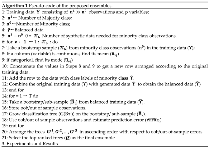
2.1. Balancing the Training Data
2.2. Out-of-Bag based Assessment with Balanced Data
2.3. Sub-Sample based Assessment with Balanced Data
3. Simulation
4. Conclusions
Supplementary Materials
Author Contributions
Funding
Data Availability Statement
Acknowledgments
Conflicts of Interest
References
- Weiss, G. M. (2004). Mining with rarity: a unifying framework. ACM Sigkdd Explorations Newsletter, 6(1), 7-19. [CrossRef]
- Parmar, J.; Chouhan, S.S.; Raychoudhury, V.; Rathore, S.S. Open-world Machine Learning: Applications, Challenges, and Opportunities. ACM Comput. Surv. 2023, 55, 1–37. [CrossRef]
- Wang, L.; Han, M.; Li, X.; Zhang, N.; Cheng, H. Review of Classification Methods on Unbalanced Data Sets. IEEE Access 2021, 9, 64606–64628. [CrossRef]
- de Giorgio, A.; Cola, G.; Wang, L. Systematic review of class imbalance problems in manufacturing. J. Manuf. Syst. 2023, 71, 620–644. [CrossRef]
- Kotsiantis, S., Kanellopoulos, D., & Pintelas, P. Handling imbalanced datasets: A review, gests international transactions on computer science and engineering 30 (2006) 25–36. Synthetic Oversampling of Instances Using Clustering.
- Visa, S., & Ralescu, A. (2005, April). Issues in mining imbalanced data sets-a review paper. In Proceedings of the sixteen midwest artificial intelligence and cognitive science conference (Vol. 2005, pp. 67-73). sn.
- Monard, M. C., & Batista, G. E. A. P. A. (2002). Learning with skewed class distributions. Advances in Logic, Artificial Intelligence and Robotics, 85, 173-180.
- Prince, M.; Prathap, P.M.J. An Imbalanced Dataset and Class Overlapping Classification Model for Big Data. Comput. Syst. Sci. Eng. 2023, 44, 1009–1024. [CrossRef]
- Kotsiantis, S. B., & Pintelas, P. E. (2003). Mixture of expert agents for handling imbalanced data sets. Annals of Mathematics, Computing & Teleinformatics, 1(1), 46-55.
- Improving identication of di cult small classes by balancing class distribution. In Articial Intelligence in Medicine: 8th Conference on Articial Intelligence in Medicine in Europe, AIME 2001 Cascais, Portugal, July 14, 2001, Proceedings 8, pages 6366. Springer, 2001.
- Han, H.; Wang, W.Y.; Mao, B.H. Borderline-SMOTE: A new over-sampling method in imbalanced data sets learning. In Proceedings of the International Conference on Intelligent Computing, Hefei, China, 23–26 August 2005; Springer: Berlin/Heidelberg, Germany, 2005; pp. 878–887. [CrossRef]
- Han, H., Wang, L., Wen, M., & Wang, W. Y. (2006). Oversampling Algorithm Based on Preliminary Classification in Imbalanced Data Sets Learning. Journal of computer allocations (in Chinese), 26(8), 1894-1897.
- Kubat, M., & Matwin, S. (1997, July). Addressing the curse of imbalanced training sets: one-sided selection. In Icml (Vol. 97, No. 1, p. 179).
- Chawla, N.V.; Bowyer, K.W.; Hall, L.O.; Kegelmeyer, W.P. SMOTE: Synthetic Minority Over-sampling Technique. J. Artif. Intell. Res. 2002, 16, 321–357. [CrossRef]
- Weiss, G. M. (2003). The effect of small disjuncts and class distribution on decision tree learning. Rutgers The State University of New Jersey, School of Graduate Studies.
- Weiss, G.M.; Provost, F. Learning When Training Data are Costly: The Effect of Class Distribution on Tree Induction. J. Artif. Intell. Res. 2003, 19, 315–354. [CrossRef]
- Jo, T.; Japkowicz, N. Class imbalances versus small disjuncts. ACM SIGKDD Explor. Newsl. 2004, 6, 40–49. [CrossRef]
- Batista, G.E.A.P.A.; Prati, R.C.; Monard, M.C. A study of the behavior of several methods for balancing machine learning training data. ACM SIGKDD Explor. Newsl. 2004, 6, 20–29. [CrossRef]
- Leevy, J.L.; Hancock, J.; Khoshgoftaar, T.M. Comparative analysis of binary and one-class classification techniques for credit card fraud data. J. Big Data 2023, 10, 1–13. [CrossRef]
- Wongvorachan, T.; He, S.; Bulut, O. A Comparison of Undersampling, Oversampling, and SMOTE Methods for Dealing with Imbalanced Classification in Educational Data Mining. Information 2023, 14, 54. [CrossRef]
- Chaabane, I.; Guermazi, R.; Hammami, M. Enhancing techniques for learning decision trees from imbalanced data. Adv. Data Anal. Classif. 2019, 14, 677–745. [CrossRef]
- Ksieniewicz, P. (2018, November). Undersampled majority class ensemble for highly imbalanced binary classification. In Second International Workshop on Learning with Imbalanced Domains: Theory and Applications (pp. 82-94). PMLR.
- Du, H.; Zhang, Y.; Zhang, L.; Chen, Y.-C. Selective ensemble learning algorithm for imbalanced dataset. Comput. Sci. Inf. Syst. 2023, 20, 831–856. [CrossRef]
- Jordan, M.I.; Mitchell, T.M. Machine learning: Trends, perspectives, and prospects. Science 2015, 349, 255–260. [CrossRef]
- Sebbanü, M., NockO, R., Chauchat, J., & Rakotomalala, R. (2000). Impact of learning set quality and size on decision tree performances. IJCSS, 1(1), 85.
- Khan, Z., Gul, A., Mahmoud, O., Miftahuddin, M., Perperoglou, A., Adler, W., & Lausen, B. (2016). An ensemble of optimal trees for class membership probability estimation. In Analysis of Large and Complex Data (pp. 395-409). Springer International Publishing. [CrossRef]
- Khan, Z.; Gul, A.; Perperoglou, A.; Miftahuddin, M.; Mahmoud, O.; Adler, W.; Lausen, B. Ensemble of optimal trees, random forest and random projection ensemble classification. Adv. Data Anal. Classif. 2019, 14, 97–116. [CrossRef]
- Efron, B., & Tibshirani, R. (1997). Improvements on cross-validation: the 632+ bootstrap method. Journal of the American Statistical Association, 92(438), 548-560. [CrossRef]
- Adler, W.; Lausen, B. Bootstrap estimated true and false positive rates and ROC curve. Comput. Stat. Data Anal. 2009, 53, 718–729. [CrossRef]
- Johnson, R.W. An Introduction to the Bootstrap. Teach. Stat. 2001, 23, 49–54. [CrossRef]
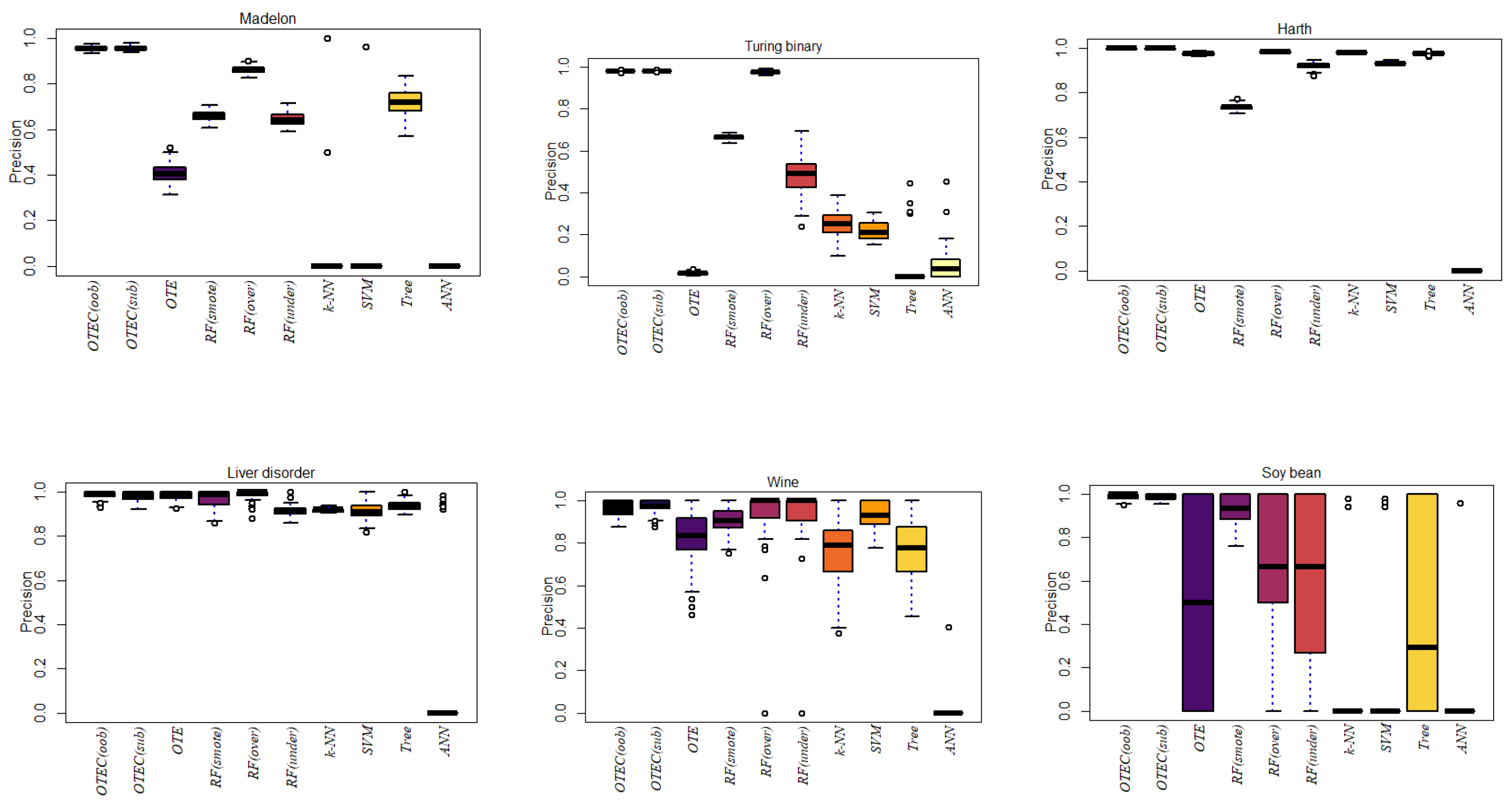
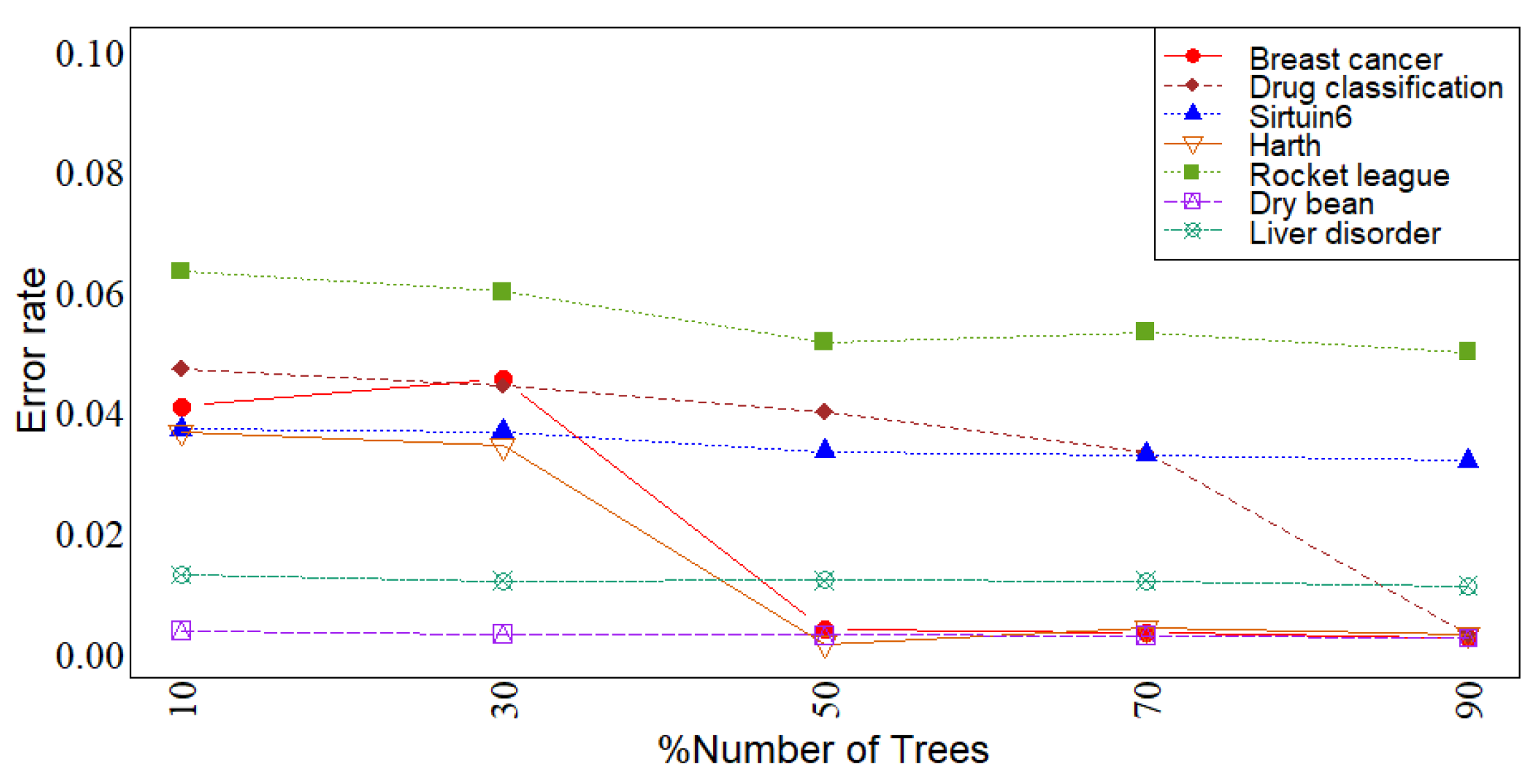
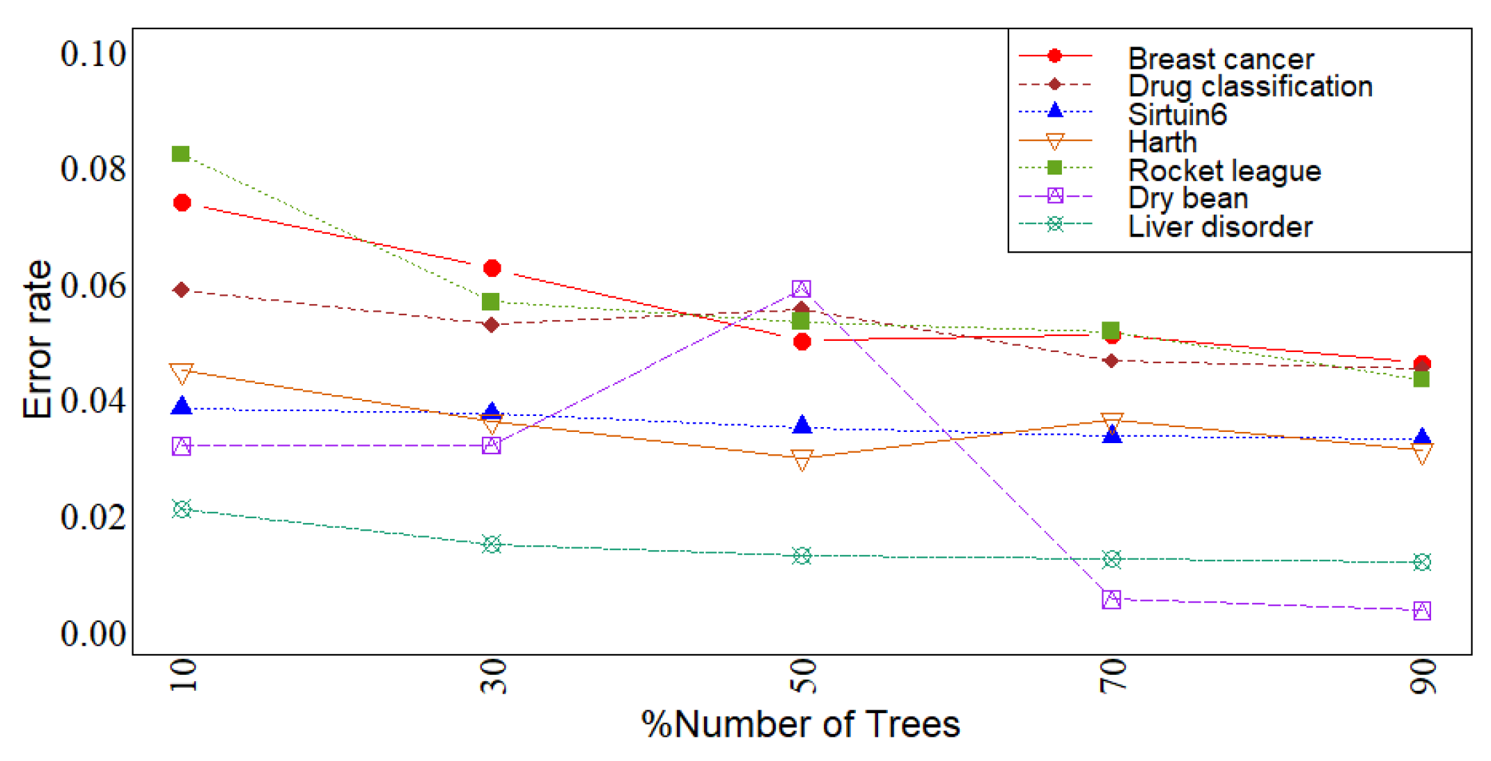

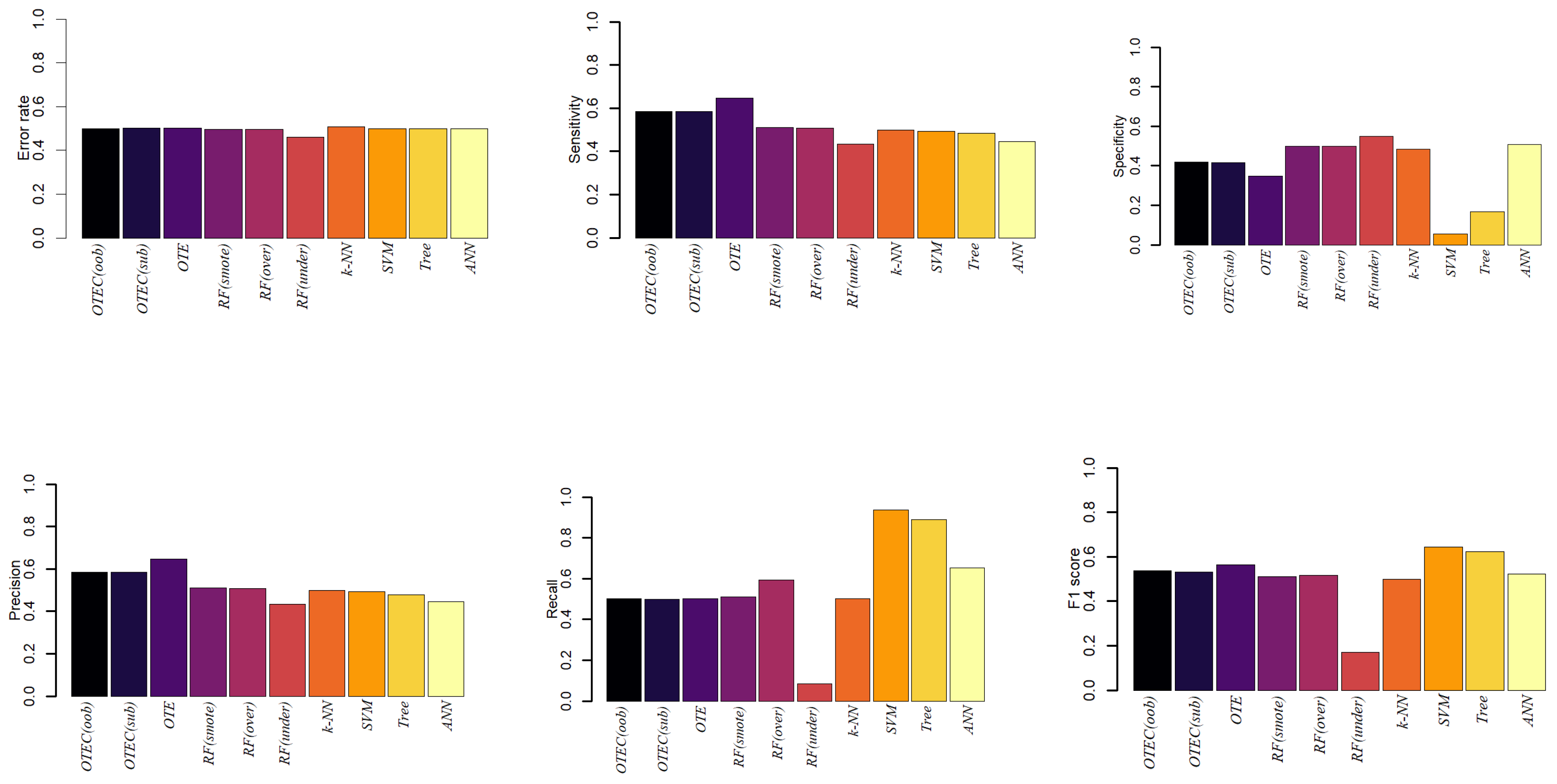
| No | Dataset | Instances | Features | Class-Based Distribution |
Imbalance Ratio n 1/n 0 |
Source |
|---|---|---|---|---|---|---|
| 1 | Breast Cancer | 569 | 31 | 357/212 | (1.6839:1) | https://www.kaggle.com/datasets/utkarshx27/breast-cancer-wisconsin-diagnostic-dataset |
| 2 | Credit Card | 284807 | 30 | 284807/492 | (578.876:1) | https://www.kaggle.com/datasets/mlg-ulb/creditcardfraud |
| 3 | Drug Classification | 200 | 6 | 145/54 | (2.685:1) | https://openml.org/search?type=data&status=active&id=43382 |
| 4 | Kc2 | 520 | 21 | 414/106 | (3.905:1) | https://openml.org/search?type=data&status=active&sort=runs&id=1063 |
| 5 | Eeg eye | 5856 | 14 | 5708/148 | (38.567:1) | https://openml.org/search?type=data&status=active&sort=runs&id=1471 |
| 6 | Glass Classification | 213 | 9 | 144/69 | (2.086:1) | https://openml.org/search?type=data&status=active&id=43750 |
| 7 | Pc4 | 1339 | 37 | 1279/60 | (21.316:1) | https://openml.org/search?type=data&status=active&sort=runs&id=1049 |
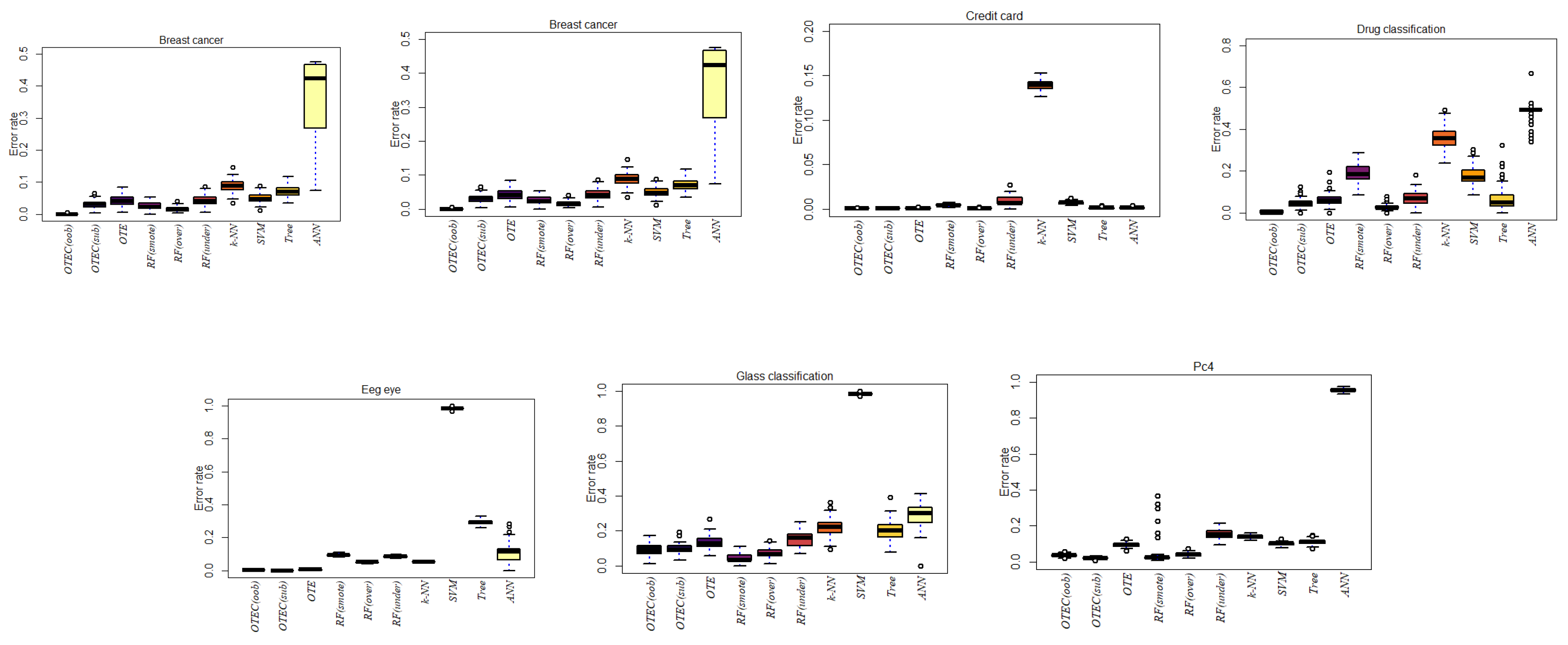
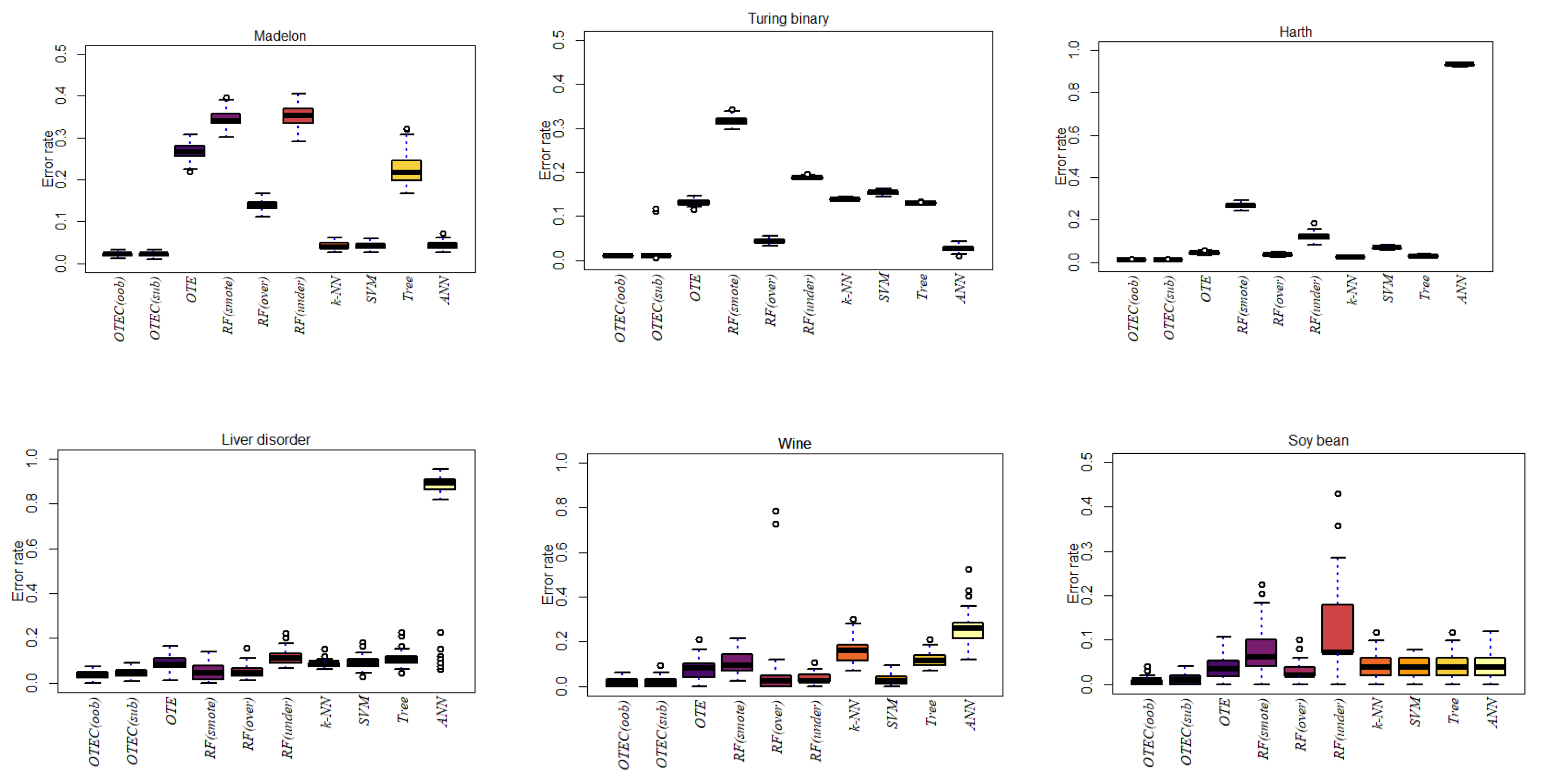
| Dataset | OTEC(oob) | OTEC(sub) | OTE | RF(smote) | RF(over) | RF(under) | k-NN | SVM | ANN | Tree |
|---|---|---|---|---|---|---|---|---|---|---|
| Breast Cancer | 0.0015 | 0.0311 | 0.0427 | 0.0264 | 0.0166 | 0.0422 | 0.0851 | 0.0486 | 0.3625 | 0.0723 |
| Credit Card | 0.0005 | 0.0005 | 0.0010 | 0.0046 | 0.0006 | 0.0083 | 0.1395 | 0.0071 | 0.0016 | 0.0014 |
| Drug Classification | 0.0038 | 0.0461 | 0.0624 | 0.1875 | 0.0296 | 0.0650 | 0.3542 | 0.1771 | 0.4998 | 0.0697 |
| Kc2 | 0.0093 | 0.0099 | 0.1743 | 0.0213 | 0.0213 | 0.2060 | 0.1579 | 0.9943 | 0.1925 | 0.1735 |
| Eeg eye | 0.0035 | 0 | 0.0063 | 0.0942 | 0.0521 | 0.0872 | 0.0553 | 0.9827 | 0.1094 | 0.2947 |
| Glass Classification | 0.0914 | 0.0974 | 0.1330 | 0.0405 | 0.0710 | 0.1518 | 0.2194 | 0.9839 | 0.2879 | 0.1993 |
| Pc4 | 0.0384 | 0.0213 | 0.0945 | 0.0411 | 0.0421 | 0.1519 | 0.1392 | 0.1006 | 0.9555 | 0.1120 |
| Madelon | 0.0222 | 0.0218 | 0.2675 | 0.3459 | 0.1397 | 0.3525 | 0.0416 | 0.0420 | 0.0435 | 0.2260 |
| Turing binary | 0.0102 | 0.0214 | 0.1321 | 0.3173 | 0.0437 | 0.1882 | 0.1392 | 0.1541 | 0.0271 | 0.1303 |
| KDD | 0.0099 | 0.0101 | 0.0355 | 0.1394 | 0.0098 | 0.1191 | 0.0198 | 0.0226 | 0.9804 | 0.0185 |
| Liver disorder | 0.0400 | 0.0453 | 0.0864 | 0.0469 | 0.0512 | 0.1153 | 0.0862 | 0.0915 | 0.7661 | 0.1126 |
| Wine | 0.0227 | 0.0173 | 0.0796 | 0.1029 | 0.0680 | 0.0324 | 0.1605 | 0.0305 | 0.2574 | 0.1235 |
| Soy bean | 0.0093 | 0.0100 | 0.0364 | 0.0706 | 0.0308 | 0.1229 | 0.0416 | 0.0420 | 0.0428 | 0.0402 |
| Ionosphere | 0.0429 | 0.0172 | 0.1168 | 0.2830 | 0.0985 | 0.1531 | 0.1107 | 0.0898 | 0.8913 | 0.1093 |
| Room Occupancy | 0 | 0 | 0.0002 | 0.0034 | 0.0003 | 0.0020 | 0.0001 | 0.00001 | 0.0211 | 0.0002 |
| Harth | 0.0121 | 0.0119 | 0.0438 | 0.2698 | 0.0379 | 0.1214 | 0.0253 | 0.0682 | 0.9318 | 0.0303 |
| Rocket League | 0.0334 | 0.0331 | 0.1032 | 0.4525 | 0.0914 | 0.1158 | 0.0622 | 0.0616 | 0.0614 | 0.0613 |
| Sirtuin6 | 0.0516 | 0.0516 | 0.2433 | 0.2680 | 0.1200 | 0.3275 | 0.0700 | 0.0965 | 0.6519 | 0.0847 |
| Toxicity | 0.0339 | 0.0352 | 0.1241 | 0.3828 | 0.1392 | 0.2750 | 0.0645 | 0.0570 | 0.0694 | 0.0692 |
| Dry bean | 0.0030 | 0.0035 | 0.0102 | 0.0500 | 0.0075 | 0.0134 | 0.0301 | 0.0103 | 0.0295 | 0.0091 |
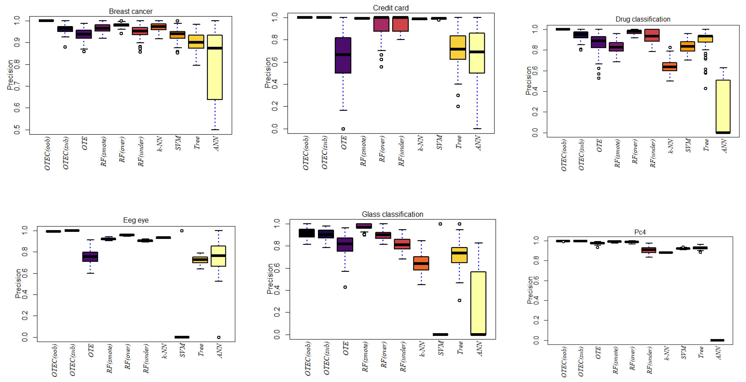
| Dataset | OTEC(oob) | OTEC(sub) | OTE | RF(smote) | RF(over) | RF(under) | k-NN | SVM | ANN | Tree |
|---|---|---|---|---|---|---|---|---|---|---|
| Breast Cancer | 1.0000 | 0.9629 | 0.9364 | 0.9670 | 0.9795 | 0.9517 | 0.9696 | 0.9353 | 0.7200 | 0.9029 |
| Credit Card | 0.9993 | 0.9992 | 0.6503 | 0.9923 | 0.9241 | 0.9505 | 0.9860 | 0.9889 | 0.6123 | 0.7284 |
| Drug Classification | 1.0000 | 0.9378 | 0.8655 | 0.8277 | 0.9714 | 0.9361 | 0.6401 | 0.8328 | 0.2006 | 0.9031 |
| Kc2 | 0.9267 | 0.8698 | 0.4658 | 0.9572 | 0.9996 | 0.6335 | 0.4017 | 0.1900 | 0.1407 | 0.5908 |
| Eeg eye | 0.9929 | 1 | 0.7578 | 0.9216 | 0.9576 | 0.9049 | 0.9327 | 0.0700 | 0.6646 | 0.7257 |
| Glass Classification | 0.9153 | 0.9022 | 0.8050 | 0.9739 | 0.8984 | 0.8166 | 0.6440 | 0.1300 | 0.2665 | 0.7204 |
| Pc4 | 0.9981 | 0.9971 | 0.9755 | 0.9904 | 0.9885 | 0.9059 | 0.8811 | 0.9207 | 0 | 0.9287 |
| Madelon | 0.9554 | 0.9563 | 0.4063 | 0.6586 | 0.8614 | 0.6449 | 0.1750 | 0.0192 | 0 | 0.7171 |
| Turing binary | 0.9796 | 0.9799 | 0.0162 | 0.6648 | 0.9757 | 0.4800 | 0.2519 | 0.2176 | 0.0541 | 0.0140 |
| KDD | 1 | 1 | 0.9987 | 0.8649 | 0.9896 | 0.2506 | 0.9802 | 0.9794 | 0 | 0.9830 |
| Liver disorder | 0.9860 | 0.9830 | 0.9835 | 0.9713 | 0.9835 | 0.9134 | 0.9206 | 0.9135 | 0.1604 | 0.9365 |
| Wine | 0.9584 | 0.9720 | 0.8302 | 0.9111 | 0.9187 | 0.9218 | 0.7678 | 0.9296 | 0.0041 | 0.7702 |
| Soy bean | 0.9888 | 0.9864 | 0.4845 | 0.9309 | 0.6332 | 0.5975 | 0.0286 | 0.0288 | 0.0096 | 0.3968 |
| Ionosphere | 0.9733 | 0.6763 | 0.9292 | 0.7239 | 0.9589 | 0.9209 | 0.8954 | 0.9137 | 0 | 0.9397 |
| Room Occupancy | 1 | 1 | 0.9971 | 0.9962 | 0.9971 | 0.9936 | 0.9943 | 1 | 0 | 0.9948 |
| Harth | 0.9980 | 0.9976 | 0.9750 | 0.7336 | 0.9828 | 0.9190 | 0.9800 | 0.9317 | 0 | 0.9749 |
| Rocket League | 0.9336 | 0.9362 | 0.0759 | 0.5431 | 0.3916 | 0.0890 | 0.1240 | 0 | 0 | 0 |
| Sirtuin6 | 0.9554 | 0.9589 | 0.6373 | 0.7638 | 0.9509 | 0.7683 | 0.9200 | 0.9235 | 0 | 0.9182 |
| Toxicity | 0.9323 | 0.9314 | 0.0386 | 0.5924 | 0.4527 | 0.1049 | 0.0100 | 0 | 0 | 0 |
| Dry bean | 0.9961 | 0.9952 | 0.8161 | 0.9503 | 0.9639 | 0.9702 | 0.0353 | 0.9283 | 0 | 0.8880 |
Disclaimer/Publisher’s Note: The statements, opinions and data contained in all publications are solely those of the individual author(s) and contributor(s) and not of MDPI and/or the editor(s). MDPI and/or the editor(s) disclaim responsibility for any injury to people or property resulting from any ideas, methods, instructions or products referred to in the content. |
© 2024 by the authors. Licensee MDPI, Basel, Switzerland. This article is an open access article distributed under the terms and conditions of the Creative Commons Attribution (CC BY) license (http://creativecommons.org/licenses/by/4.0/).


