
Submitted:
23 July 2024
Posted:
23 July 2024
You are already at the latest version
Abstract
The repeated application of herbicides has led to the development of herbicide resistance. Models are useful for identifying key processes and understanding the evolution of resistance. This study developed a spatially explicit model at a landscape scale to examine the dynamics of Lolium rigidum populations in dryland cereal crops and the evolution of herbicide resistance under var-ious management strategies. Resistance evolved rapidly under repeated herbicide use, driven by weed fecundity and herbicide efficacy. Although fitness costs associated with resistant plants re-duced resistance evolution, they did not affect the speed of spread. The most effective strategies to slow resistance involved diversifying cropping sequences (e.g., crop rotation) and the herbicide applications (e.g., rotating different herbicide modes of action). Pollen flow was the main disper-sal vector, with seed dispersal also contributing significantly. Strategies limiting seed dispersal effectively decreased resistance spread. However, the use of a seed-catching device at harvest could unintentionally enrich resistance in the area. It would be beneficial to optimise the move-ment of harvesters between fields. The model presented here is a useful tool that may assist in the exploration of novel management strategies within the context of site-specific weed management at the landscape scale, as well as in the advancement of our understanding of resistance dynamics.
Keywords:
explicit genotype mode
; dispersal vectors
; gene flow
; population dynamics
; operational factors
; spatially explicit model
1. Introduction
Weeds are widespread on farmland in all regions of the world. They compete with crops for space and resources and decrease yields because of their competitive capacity and abundance [1]. This makes them undesirable and efforts to control weeds are often based on herbicide applications [2] often with the same mode of action year after year [3]. If herbicide resistant (HR) genotypes are present in populations, the high selection pressure exerted by these applications in will result in the evolution of herbicide resistance [4]. Currently, there are more than 300 herbicide resistant biotypes currently documented [5]. Lolium rigidum (Gaud.), an important annual weed in Mediterranean cereals, evolving resistance to 14 different herbicide groups [6,7]. The first case of an herbicide resistant L. rigidum Gaud. population was reported by [8], with resistance reported to chlortoluron (PSII inhibiting herbicide) and diclofop-methyl (ACCase inhibiting herbicide) Resistance to ACCase, ALS and PSII inhibitors is now widespread throughout the Spanish winter cereal cropping system [9,10].
To better understand and identify the key process affecting herbicide-resistance evolution a large number of models have been developed (see [11]). Models are useful tools to facilitate the study of weed population dynamics over a long period of time at different spatial scales. Important factors that impact on the rate of resistance evolution include the weed biology, the genetics of the resistance genes, and herbicide and cropping system parameters [4,12]. Essential components of the model are consequently based on the knowledge about these factors and their interactions and are reflected on the structure of the model. Hence, a model could include a population genetic, a weed population dynamic and a dispersal submodel [13]. The weed population dynamic submodel relies on the biology of the weed such as the germination pattern, the dormancy, the seedling survival and the seed production whilst the genetic submodel deals with the inheritance of the herbicide-resistance trait. Finally, a spatial dimension of the model cannot be omitted because of the importance of the pollen and seed flow on the evolution and spread of resistance [14]. A reduced number the models have examined spatial aspects of herbicide resistance evolution [15,16,17,18,19,20]. Most of these models construct theoretical frameworks where management scenarios to slow resistance spread are simulated. Management strategies are studied either at the temporal scale, i. e. the management scenarios take into account diversified control methods over time [15] or at a spatio-temporal scale, i. e. the spatial organization of the control methods is also included [18,19].
The spatial processes that result in the evolution and spread of herbicide-resistant plants are affected by diverse factors such as landscape connectivity and the distance among donor areas and areas suitable for invasion. These processes are defined by the landscape composition and biological characteristics associated with weed spread. In most previous approaches, a homogeneous landscape with equal field size, shape and distribution was considered [18]. This approach is achieved using cellular automata which have a simple grid structure making models easy to implement. Another more complex approach adopts a polygonal approach to landscape composition [19]. In this case, the sizes, the shapes and the distances among polygons (i. e. fields) are not homogeneous and the distribution over space is normally that outlined from a particular landscape. We have adopted a mixed approach based on a cellular automaton grid whereby cells are aggregated to match real field size distributions for a particular study site. So, we have a heterogeneous landscape with different field sizes and distances among fields easily changeable according to the landscape structure. Taking into account these particular attributes, a spatially explicit model was developed in order to create a framework whereby the dispersal events associated with pollen and seed movement of herbicide-resistant L. rigidum are included according to the biology and ecology of the weed and the landscape in the South of Spain.
The objectives of this study were: i) develop a spatially-explicit weed model of HR evolution of L. rigidum, ii) Use this model to simulate HR evolution under current cropping regimes and diverse management strategies to slow down HR evolution, iii) Identify the dispersal vectors that mainly drive HR evolution at the landscape level and iv) the key parameters that most influence model outcomes.
2. Materials and Methods
2.1. Model Description
The spatially explicit model was constituted as a regular grid consisting of R x R cells with R=100. Each cell represented a farm field of 1 ha in which an independent weed seed population developed. So, the simulated landscape was an area of 10000 ha which can be thought of as a portion of the agricultural dryland area of Andalusia (South of Spain). The R cells were spatially aggregated into larger units called fields. All of the unit cells of a simulated field follow the same management program and consequently they are exposed to equal selection pressure. Eight possible size classes were considered in the model (Table 1). The number of fields in each field-size class accounted for the current field-size distribution in the Andalusian landscape both in terms of the number of fields and the total area occupied by a particular field-size class. Such cell aggregation followed specific rules such a rectangular shape (5:4 or the nearest possible) [21], similar to those found in many European countries. Field allocation was randomized over the landscape in order of decreasing field size. An example of the simulated landscape is depicted in the Figure 1. As this routine makes the model stochastic each simulation scenario was replicated 100 times.
The crops included in the model were those most abundant in the Andalusia farmland [22]: cereal and sunflower. Cereal crops are sown in monoculture or in cereal-sunflower two-year rotations. Sunflower crops are always sown in rotation with cereals. Around 58% of the whole landscape was under cereal monoculture and the remaining 42% was under cereal-sunflower rotation. The initial assignment of both crops over the simulated landscape was randomized according to the current area distribution (Table 1).
A population dynamics submodel was implemented in each cell. Processes of interchange of L. rigidum pollen and seeds between cells allow gene flow over the landscape and these processes are included as another submodel. Both submodels are addressed in depth later and are schematized in Figure 2.
2.2. Population Dynamic Submodel
The population dynamic submodel combines a weed population dynamic and a single-gene explicit genotype model. The first describes the weed life cycle and the second is a population genetic model whereby the frequency of individual herbicide susceptible and herbicide resistant genotypes is accounted. The herbicide-resistance gene is a major nuclear dominant gene with two alleles denoted by ‘A’ and ‘a’, i. e. ‘A’ codes for resistance and ‘a’ for susceptibility to herbicides. Then, we would have three possible genotypes: homozygous susceptible (aa), heterozygous resistant (aA) and homozygous resistant (AA).
The weed population dynamic submodel was parameterized for L. rigidum and accounts for the main states of the weed life cycle. Such states are interconnected by fluxes derived from the weed biology itself and operational events in the crop (Figure 2).
2.2.1. Seed Bank Dynamic and Seedling Survival
The model has a depth-structured seed bank in three different soil layers. The first layer constitutes the surface to 5 cm depth, the second layer from 5 cm to 10 cm depth and the final layer deeper than 10 cm. At the beginning of the simulations, the total initial weed seed density (SBini) in the soil was concentrated in the first soil layer with the genotype frequencies based on Hardy-Weinberg equilibrium [4] calculated according to an initial frequency of the herbicide resistance allele, pini.
A model simulation year starts in August with a new cropping season and finishes with the crop harvest in July of the following year. As the weed seed bank is a depth-structured variable the model was organized in terms of matrices with a structure similar to that used in the model developed by [15]. Then, the weed life cycle main stages for each genotype can be represented as a state vector whereby its components are the seed bank in each soil layer (SB1, SB2, SB3), the seedlings (SL), the adult plants (AD) and the seed rain (SR). The state vector in each cell position [i, j], , is indexed by the time step in the life cycle evolution (subscript y) within every model simulation year (superscript t) and genotype (subscript xx, with values aa, aA and AA).
The initial weed population structure at the beginning of the cropping season is that at the end of the previous cropping season .
The exchange of seeds between soil layers and the death of established seedlings result from the tillage operations related to the crop grown during each year. The matrix which accounts for these processes is denoted by Tl,n with l being 1, 2 or 3 with regard to the order of the tillage event during the cropping season. The elements of the matrix T are indexed by the subscript n which means the crop to be grown in the current cropping season with values 1 and 2 for cereal and sunflower crops, respectively.
A primary soil cultivation to incorporate the stubble from the previous crop harvest is a common crop-related operation in Andalusia that facilitates the weed seed movement into the soil. A disc and a paraplow are the tillage tools usually used for cereal and sunflower crops respectively [23].
With
The matrix elements t1 are indexed by the source and recipient soil layer in the seed movement, e. g. t132 is the fraction of seeds coming from the soil layer 3 to the soil layer 2 as a consequence of the first soil cultivation.
Seed removal from the shallow soil layer by harvester ants may have a large impact in decreasing the weed seed bank size in dryland cereals [24]. The weed seed removal rate by the predation activity is included in the model as element d of the projection matrix D.
With
L. rigidum has a germination period focused on the winter season and mainly associated with cereal crop germination time with some weed plants already established at crop seeding time [25]. Hence, we distinguish two cohorts in relation to crop seeding event. Seedlings of cohort 1 are those that germinate prior to crop seeding and are affected by a second tillage event with a field cultivator or a deeper tillage with a scarifier in fields where cereal or sunflower crops are expected to be grown [23]. The seed bank and the established seedlings are affected as follows
With
and
The fraction of the seed bank that remains in the soil or germinates in each soil layer is given in the germination matrix G1 (indexed by the cohort) by the expressions (1- g · c1) and (g · c1). The proportion of overall germination, g (indexed by the soil layer position), contributed by cohort 1 is denoted by the constant c1 with s2 the fraction of seedlings surviving the second mechanical control.
A common practice for farmers is to sow a fraction of cereal seeds from the previous harvested crop [26,27]. This crop seed may have been contaminated with weed seeds that increase the weed seed bank in the first soil layer. The weed seeds contaminating the crop seeds to be sown in a field are denoted by CCG and it corresponds with a fraction of weed seeds contaminating the cereal seeds from the previous harvested cereal crop in such field. The matrix which accounts for this process is denoted by
Once the weed cohort 2 has germinated the established weed seedlings of both cohorts are controlled according to the crop sown in the field; mechanical control in sunflower crops and chemical control by post-emergence herbicide application in cereal crops. The fraction of the seedlings that survives to the post-emergence herbicide application is given in the matrix Hn (indexed by the crop). The seed bank and seedlings surviving these control methods are
With
And
And
With c2 being the proportion of overall germination contributed by the cohort 2 and s3n and hn,xx the survival fraction following mechanical and chemical control, respectively. The control exerted by the herbicide on each of the three weed genotypes can be different and reflects dominance and fitness in the presence of the herbicide.
As no density-dependent mortality has been observed for L. rigidum seedlings [28] a fixed proportion v of total established seedlings reaches maturity. The projection matrix V accounts for natural seedling survival.
With
2.2.2. Seed Production
The established mature individuals produce haploid ova (unfertilized seeds) and pollen in relation to their own genotype. Ova are produced by adult plants in direct proportion to predicted seed production (see below) and pollen is produced by individual plants in excess. The pollen produced in each cell and the pollen that is dispersed into the cell by pollen flow from neighboring cells fertilizes the ova present to produce seed of the three resistance genotypes.
We denoted the amount of ovules (seeds) produced by the adult plants as OVxx[i, j] with genotype xx according to a density-dependent hyperbolic model fitted to L. rigidum [28].
With
The total seed rain, SRtotal[i, j], is
The frequency of the herbicide-resistant and herbicide-susceptible allele, p and q respectively, of the produced ova is estimated as
These frequencies can be modified by spontaneous mutation at the locus coding for herbicide resistance. The mutation rate is k and the new frequencies of the resistance alleles, pm and qm, are
If we denote ppo[i, j] and qpo[i, j] as the frequency for each allele in the pollen cloud of a particular cell, which takes into account pollen movement (see later), and assuming that L. rigidum is an obligated outcrossing species, the genotype frequency of the seed rain, GFxx, after the mating is calculated as follows
After mating, the already produced seed rain is incorporated into the system, matrix Fxx. The mortality of the seed bank during the cropping season is denoted by the matrix M. The state vector at this point is
With
And
The natural mortality of ungerminated seeds is denoted by m1, m2 and m3, i. e. the fraction of seed removal in the first, second and third soil layer.
Finally, the new produced seeds are incorporated to the soil surface finishing the weed life cycle in the detailed cropping season.
With
As described above, movement of seeds between cells by the harvester is avoided and every weed seed is dispersed in the cell where it was produced. Weed seed movement over the landscape by the harvester is further detailed in the gene flow submodel.
2.3. Gene Flow Submodel
Gene flow and consequently herbicide resistance dispersal over the landscape can be driven by two long-distance dispersal sources: pollen and seeds. The maximum distance and the shape of the dispersal distribution for pollen and seeds depend on the dispersal agent i. e. wind and agricultural machinery for L. rigidum pollen and seeds, respectively.
2.3.1. Pollen Dispersal
The pollen is dispersed around a focal cell following the von Moore neighborhood method [15], i. e. a central cell spreads pollen grains to its eight neighboring cells. The Moore radius, denoted by r in equation (19) takes values from 1 to z, a value of 1 indicating that pollen is spread to directly neighboring cells only and where z is the maximum of rings of cells that the pollen cloud disperses to. Therefore, the pollen quantity received by a cell in the landscape, PO, is weighted by its distance from all pollen-donating cells with this pollen cloud being mainly composed of pollen grains from the closest cells. The pollen is spread isotropically to the cells belonging to the same ring.
With pol0, pol1, …,polz the weighting factor of the pollen coming from cells belonging to a particular ring in the pollen cloud.
We supposed that the proportion of resistant alleles in the produced ova and pollen was equal and based on the proportions of mature plant genotype in a given cell. Hence, the pm and qm values are equal for the produced ova and pollen. The frequency of the resistance alleles in the pollen for a cell, ppo and qpo, is a weighted sum of the frequency of the resistance alleles in the pollen cloud for such cell,
2.3.2. Seed Movement
Weed seed movement over the landscape may occur via two mechanisms, both originating from the crop harvest. These are seed dispersal as a result of harvester movement between cereal cells and seed dispersal between cells of the same field as a result of sowing weed-contaminated cereal grain obtained from the harvested cereal crop in the previous cropping season.
2.4. Harvesting Cereal Crops
The fate of newly produced seeds depends on the timing of seed maturation. Seeds dropping earlier from the mother plant will be immediately incorporated into the shallow layer of the seed bank (SB1) of the current cell while later-ripening seeds may be harvested with the cereal crop and dispersed by the harvester or as contaminants of cereal grain. We denoted the fraction of produced seeds entering the harvester as gat. A fraction of these seeds will become mixed with the cereal grain (con), while the remainder will be returned to the soil surface following dispersal by the harvester. Dispersal by the harvester will result in seed being returned to the soil surface in cells distant from where they were produced. In our model the fraction of produced seeds exported from a cell are denoted by ES and CG, for seed dispersal vectored by movement of the harvester or seed contamination, respectively. The variable IS represents the seeds imported into the current cell coming from the previous harvested cell and it is equivalent to the ES fraction exported from such previous harvested cell. The state vector Z9 is rewritten to include the weed seed dispersal at the harvest timing.
With
and
With expt the fraction of seed exported from one cell to the next by the harvester. The position of the previous harvested cell according to the harvester movement is denoted by the coordinates [ihar-1, jhar-1]. In the model, the harvester movement is similar to the LOCAL harvesting procedure from [21]. The harvester driver knows the harvesting area and minimizes the movement between cereals fields (i. e., choosing the nearest cereal fields).
2.5. Sowing Weed-Contaminated Grain
The extent of crop grain contamination with weed seed is calculated on a per field basis as the average of contamination in all cells harvested in that cereal field. A fraction of this cereal crop seed may then be sown in the following cereal cropping season in the same field where it was harvested. The potential weed seeds to contaminate the cereal cells at the following seeding timing, CCG1, would be described as follows
With sr the seeding density and yield the expected cereal yield. Denoted by size is the field size or cell number of the field under consideration. The coordinate [i, j]e refers to the position of the cells into the equal field. In sunflower cells equation (26) take the value of zero, CCG2=0.
2.6. Stochastic Routines
To avoid overestimates of herbicide resistance evolution resulting from the inclusion of fractional seeds and plants in the weed life cycle (see [29]) values were rounded to an integer according to the method of [30], such that
with U a random number between zero and one and X the outputs, i. e. adult plants, AD[i, j], and seed rain, SR[i, j].
2.7. Parameters of the Model and Initial Conditions
The parameters used in the model are listed in the Table 2 according to the data coming from the literature. As far as possible, the parameter values were taken from Spanish data sets to get a more accurate description of the environment where the model was developed.
2.8. Simulation Scenarios
The model was used to study a variety of management scenarios to predict evolution of herbicide-resistance in L. rigidum populations. The influence of biological, ecological and genetic factors was also investigated in order to best understand the herbicide resistance behavior at the farmland scale. The outputs were analyzed based on the dynamics of herbicide resistance evolution, i. e., the total weed seed bank and the phenotypic frequency of herbicide resistance averaged over the landscape. The spatial spread of herbicide resistance was studied based on the area occupied by weed populations with evolved resistance (i. e., more than 20% of the seed bank is herbicide resistant; [42]). The relative importance of each dispersal vector in herbicide resistance spread was studied in a sequence of separate simulations and dispersal patterns were compared.
2.8.1. Section 1: Evolution of the herbicide-resistant L. rigidum Populations
Predictions for herbicide resistance evolution were simulated with the parameters and initial conditions fixed to the default values and the management system given in the model procedure (scenario = EST 0). Cereal crop seed sown in all fields was a portion of that which was harvested in the previous year in that field (certified seed was not sown). Parameter values in all subsequent simulations were those discussed in the preceding section and included in Table 2 unless otherwise stated.
2.8.2. Section 2: Resistance Management Strategies
Management strategies to delay the evolution and dispersal of herbicide resistance can be thought as strategies carried by farmers individually at the field level but with landscape effects. These strategies arise from two general groups of measures: decreasing selection for resistance by diversifying weed control methods and/or slowing herbicide resistance spread. In the first group of measures we consider both an increasing farming area with crop rotation and the rotation of different herbicide modes of action among years. The fraction of fields over the whole landscape with a crop rotation program (EST 1) i. e., cereal-sunflower rotation, was implemented in the 100% of the landscape. Cereal crop was grown as the starting crop in year 1 in half of the simulated fields and sunflower crop was grown as the starting crop in year 1 in the remainder fields. Herbicide rotation in cereal crops through the use of alternative modes of action were implemented at random in 50 and 100% of the landscape (EST 2 and EST 3, respectively). Both herbicides were equally efficient at controlling the weed but one of them selected for the target herbicide resistance.
The second group of measures depends on the sowing of certified crop seed in the cereal cropping season for all fields in the landscape (EST 4) and the collection of the chaff ejected by the harvester (EST 5). The use of certified crop seeds is supposed to reduce in 100% the weed seeds incorporated by sowing. In EST5, when a seed catcher was connected to the harvester, the amount of seed returned to the soil surface was reduced by 66% [41]. Combinations of the single measures implemented in EST1 to EST5 (except EST2) were simulated in groups of two, three and four individual strategies as detailed in the Table 3.
2.8.3. Section 3: Importance of the Dispersal Vector in the Evolution of Herbicide Resistance
Individual simulations were conducted to establish the importance of each dispersal vector in determining the pattern and quantity of herbicide-resistance spread over the landscape. To avoid equivocal results the mutation rate was set to zero in the simulations and just one herbicide-resistant weed-infested cell (with the frequency of the herbicide-resistant allele equal to unity) was allocated in the middle of the area with equal weed density as the remainder of cells in the landscape. The dispersal vectors were: pollen flow, seed movement by sowing contaminated crop seeds and by the harvest process and all possible combinations.
Strategies based on the use of a seed catching and cleaned crop seeds for seeding were also included in an attempt to slow resistance spread. Seed cleaning operations can reduce the presence of L. rigidum seeds in crop seeds for sowing to approximately 98% [26].
2.8.4. Section 4: Sensitivity Analysis
Sensitivity analyses were performed on demographic, genetic and dispersal parameters and spatial patterns. The parameter values and the spatial patterns (i.e., model modules) to be evaluated were those known to have varying values, were difficult to estimate or were known to have a large influence on model outputs [21,28,43]. The uncertain demographic and genetic parameters were the potential fecundity, herbicide control efficacy, the mutation rate, the fitness penalty and the spatial variability of the initial conditions i. e., the initial weed density and the initial frequency of the resistant allele. These parameters were evaluated under the conditions specified in Section 1 (EST 0). The effects of the fitness penalty were included as decreased potential fecundity of resistant plants.
The uncertain dispersal parameters and spatial patterns to be evaluated in sensitivity analyses were the length of the tail of the pollen flow distribution and the pattern of harvester movement over the landscape. Both were analyzed in the context of the conditions specified in the simulations of section 3. The harvester movement over the landscape during the harvest process was changed as described by [21] to represent FOREIGN movement whereby the harvester driver did not know the working area and consequently the relative position of the cereal fields to each other.
The domain of each parameter is detailed in the Appendix A. Each parameter was evaluated independently using the default value for all others parameters in the model.
3. Results
3.1. Section 1: Evolution of Herbicide-Resistant L. rigidum
The evolution of herbicide resistance in L. rigidum populations was first observed during the third year of simulations (Figure 3) and during the next four generations the weed population became constituted completely by herbicide-resistant adult plants. The evolution pattern was similar if we focus on weed seed bank (Figure 3) but its buffer effect provoked a delayed and smoothed growth rate of the herbicide-resistant L. rigidum seed bank. This pattern is similar in others simulations although in some cases the buffer effect of the seed bank is much more evident. Because the seed bank is more stable over time than the adult plants the seed bank dynamic was chosen to explain the outcomes of the model in future simulations.
The phenotype frequency of the herbicide-resistant weed seed bank in cereal monoculture increased faster than it did in crop rotations (Figure 4) where the increase in resistance frequency oscillated and there was more than a three-year delay in reaching the maximum value.
After four years of simulations the weed population became herbicide-resistant in more than the half landscape (Figure 5 and Figure 6). A weed population was considered to be herbicide-resistant when more than 20% of its total seed bank is heterozygote or homozygote herbicide-resistant [42]. After eight generations all the fields in the landscape showed herbicide-resistant weed populations (Figure 5 and Figure 6).
3.2. Section 2: Resistance Management Strategies
3.2.1. Weed Population
The weed seed bank increased over the landscape in all individual strategies simulated (Figure 7A). The individual strategies EST 1 (increased area under crop rotation) and EST 5 (seed catching) achieved the greatest reduction in weed population growth rate over the landscape. No effect was seen in the total seed bank for EST 4 (certified-crop seed sowing) compared to the initial conditions (EST 0). The application of an herbicide with different mode of action in rotation over time in the half (EST 2) or the entire landscape (EST 3) showed an oscillatory behaviour in the seed bank evolution, and weed infestation levels halfway between strategies previously cited (Figure 7A).
The combinations of the all individual strategies were simulated and extra control of the weed seed bank was found in many cases (Figure 7B). EST 5 resulted in a decreased weed seed bank in all strategies of which it was part (Figure 7B). EST 13 and EST 16 resulted in the lowest seed banks (Figure 7B) even lower than the initial seed bank over the 20 years of simulation. Similar pattern showed the EST 11 and EST 15 during the first eight years of simulation, although after this time, the seed bank increased more than the initial seed bank. All other strategies to EST 13 and EST 16 increased the initial seed bank in different rates over the simulated period of time.
3.2.2. Resistance Frequency
The frequency of herbicide resistance increased quickly in all individual strategies (EST 1 to EST 5) simulated (Figure 8A). EST 4 and EST 5 resulted in very similar increases in herbicide resistance over time and were similar to EST 0. However, EST 1, EST 2 and EST 3 slowed resistance evolution. The time taken for 50% of the weed population to become herbicide resistant was delayed by two years for EST 2, by more than two years for EST 1 and by more than four years for EST 3. The time to reach a completely herbicide-resistant population was greater for EST 3 than for EST 1 and EST 2.
Extra control of the resistance level was found in cases where individual strategies were in combination (Figure 8B). As EST 4 and EST 5 did not show a significant reduction in resistance evolution, the double strategies which included one of these strategies (EST 7 to EST 11) and the triple strategies which included both of these strategies (EST 14 to EST 15) did not significantly improve resistance management (Figure 8B). EST 6 and EST 12 were the multiple strategies which most decreased resistance evolution over the landscape (Figure 8B). Intermediate level of control was achieved in the remainder strategies (EST 13 and EST 16).
3.2.3. Resistance Spread
With regards to the spread of the resistance, EST 4 and EST 5 resulted in herbicide resistance spreading over the half of the described landscape in 4 year time. This was observed after six-seven years for EST 1, EST 2 and EST 3. EST 2 and EST 3 predicted a five- and six-year delay in the time taken to reach the asymptote relative to EST 1 (Figure 9A).
The combinations of some individual strategies increased the control exerted in the resistance spread over the landscape (Figure 9B). As cited previously for resistance evolution, EST 4 and EST 5 did not show a significant reduction in resistance spread and consequently EST 7 to EST 11 and EST 13 to EST 14 did not significantly improve resistance management (Figure 9B). EST 6, EST 12 to EST 13 and EST 16 predicted six-year delay in the time taken to spread the observed herbicide resistance over the half of the landscape compared to the most efficient individual strategies. EST 16 which involves all individual strategies slowed the dispersal rate of the resistance over the landscape more efficiently than all strategies over the 20 years of simulation (Figure 9B).
3.3. Section 3: Importance of the Dispersal Vector in the Evolution of Herbicide Resistance
In simulations where resistance spread from a single focal cell, the influence of different dispersal vectors in resistance spread over the landscape can be analyzed over two time intervals: the short and the long term. In the short term, sowing contaminated crop seed increased the area infested by herbicide-resistant populations faster than the other vectors (Figure 10A). However, the behavior in the long term was the opposite, with pollen flow expanding the resistance problem further than contaminated crop seeding. The spread of herbicide resistance was described by an exponential and a sigmoid curve for pollen flow and crop seeding, respectively. Harvester movement resulted in a linear increase in herbicide resistance spread with lower rates of spread than the other dispersal vectors (Figure 10A).
Resistance spread a greater distance from the focal cell as a result of pollen flow then it did as a result of harvester movement (Figure 10B), although there were some large ranges of variation in the data. The weed seeds infesting the crop grain travelled furthest in the short term but spread by this vector was truncated in the long term by the impossibility of infesting new fields (Figure 10B).
A positive synergistic effect was found when including all dispersal factors together (results not shown). This synergy was greatest when pollen flow and weed contaminated-crop seed seeding were considered together. The area occupied by an herbicide resistance weed population rose by 6.8 times in this case and by 9 times when all dispersal factors were considered together with respect to simulations where pollen flow alone was considered.
3.4. Section 4: Sensitivity Analysis
The model was sensitive to the potential weed fecundity, herbicide efficacy and fitness cost parameters (Figure 11). Variations in potential fecundity had greatest impact on the model, significantly impacting the years to resistance evolution across the entire landscape (i. e., more than 20% of the total seed bank in the landscape is herbicide resistant) and the years to evolve resistance over half of the landscape (Figure 11) and both responses were not lineal. The time to resistance evolution and spread were much greater as the potential fecundity decreased. The seed bank density also highly decreased its potential value under a decreased potential fecundity (results not shown). The fitness cost and herbicide efficacy showed a linear pattern over their uncertain domains on the time to resistance evolution, although this effect was almost non-significant for the fitness cost with just a one-year delay on resistance evolution. The herbicide control did not influence the potential weed seed bank (results not shown) but it delayed the time until resistance was observed over half of the landscape by up to four years (Figure 11B). On the other hand, the fitness cost decreased the potential growth of the seed bank by up to 60% (results not shown) but it did not influence the herbicide-resistance expansion rate (Figure 11B). The model was not sensitive to the distributions of the initial weed density and the initial frequency of the resistant allele for either output analyzed (results not shown).
The distance of pollen flow had a very significant effect on the total area occupied by herbicide resistant weed populations (Figure 12A) and consequently on the distance which resistance was spread (results not shown). As the length travelled by the pollen cloud increased, the area with resistance problem at year 20 increased. The module of the model which described the harvester movement over the landscape also showed a significant effect in the model outputs (Figure 12B). The foreign movement spread the resistance over 3220 ha more and to greater distance (results not shown) than the local movement. Longer pollen distribution tails and an unknown landscape for the harvester driver increased the rate of spread and extent of herbicide resistance.
4. Discussion
Our simulations suggest that target-site herbicide resistance will evolve rapidly in weed populations with repeated annual applications of the same herbicide mode of action. In only three years, resistance was predicted over 20% of the landscape. This is in agreement with experimental results whereby herbicide-resistant L. rigidum populations became evident in the field after three consecutive years of selection with the herbicide sethoxydim [44]. Sethoxydim belongs to the cyclohexanedione (CHD) herbicides which inhibit the plastidic enzyme acetylcoenzyme A carboxylase (ACCase). The resistance evolved by repeated application of sethoxydim was endowed by a less sensitive form of ACCase [44] and therefore it was resistance attributed to target enzyme modifications. In other studies [45] frequencies up to 99% of resistant ACCase alleles were observed at field after 12 years of herbicide application in agreement with our outcomes. However, although resistance evolved very rapidly over the landscape, a farmer may not detect this problem because the number of adult plants was still low at the simulation year four (20 plants/m2).
In Spain, and particularly in Andalusia, there are reports of herbicide-resistant L. rigidum populations [46], although the evolution of resistance may have been much slower than predicted by the model. According to the sensitivity analysis, the parameters with the greatest influence on resistance evolution were the potential fecundity and herbicide efficacy. As the profits associated to cereal crops are low in some parts of the Andalusia region, this may mean that herbicides are not applied every year and there may even be rotation with fallow [2] decreasing the herbicide pressure and consequently resistance evolution. Default parameter values for fecundity were from a study in central Spain [28] where fecundity was high (935 seeds/plant). Fecundity in this region may be higher than it is in Andalusia where environmental conditions are different. This could explain in part the rapid evolution of the resistance under the conditions detailed in the model. It could be interesting to include a randomized pattern of these parameters, i. e., potential fecundity and the herbicide control rate in further models to predict the resistance appearance in L. rigidum populations in order to increase the variability in the resistance evolution over the landscape.
The rapid evolution of resistance evident in the weed adult plants was however buffered in the weed seed bank. Other models have obtained similar results [13] predicting a slower response to selection in the weed seed bank than in growing weed populations. L. rigidum is an annual weed with a seed bank living in the soil no more than two cropping seasons [25], the buffering effect of the seed bank may be increased in weeds with greater seed bank persistence whereby the time to evolve resistance could be delayed as has been shown in other modelling exercises [15].
The rate of spread of resistance was very pronounced such that after four years of simulations over half of the simulated landscape had a seed bank containing over 20% of resistant phenotypes. This value was coincident with the proportion of fields under cereal monoculture. In fields with crop rotation resistance evolved later due to a lower intensity of herbicide application. Some fields under crop rotation achieved higher levels of resistance due to stochastic dispersal events. The randomised mutation events did not show any effect (results not shown), though. However, the dispersal events were not an important impact in the model outputs as can be seen in the sensitivity analysis and the management scenarios (EST 4 and EST 5). The source of the resistance and its rapid expansion over the landscape was probably due to the large size of the individual cells explored and consequently the high initial weed density at this scale compared to the initial frequency of the resistant allele. The initial frequency of resistance and large population sizes, both resulted in resistance appearing during the first year of simulations in the seed bank of every field. Although [45] proposed multiple independent appearances of mutant ACCase alleles in a region as the origin of the herbicide-resistant Alopecurus myosuroides populations rather than resistance dispersal, other studies show a more important role of the gene flow in resistance expansion [14]. In our model, the weed infestation was homogeneously distributed within the 1 ha field but it is known that weeds are commonly grouped into patches although L. rigidum populations do not usually show persistent patches over time [47]. In reality, this may decrease the initial weed density at the beginning of simulations and consequently the resistance appearance and its rapid evolution within the field. Further work increasing the spatial variability of such parameters and decreasing the initial density and the initial frequency of resistance in order to reduce the probability of resistance appearance over the landscape are also recommended to create a stochastic mosaic of resistance which is more realistic. [15] and [48] showed two different approaches to get a variance in the initial starting frequency of resistance among fields.
The magnitude and existence of fitness costs associated with herbicide resistance in L. rigidum populations remain unclear and may vary depending on the type of resistance mechanism [49]. In the model, a fitness cost had a significant influence on the model outcomes. It was included in the model as a reduction in the fecundity of the homozygous herbicide-resistant weeds, however, fitness costs and trade-offs could affect many processes in the weed life cycle [50,51] found a different seed dormancy and germination dynamics in the fraction of L. rigidum weed seeds with the Ile-1781–Leu ACCase mutation. Although this is not a fitness cost per se this behavior may be important in the management of resistance evolution [50]. A relationship between dormancy and herbicide resistance has been observed by other authors [34]. We ran an extra simulation with a modified pattern in the germination of the herbicide-resistant weed seeds (a reduction of 40% and 20% in the germination for the first and the second soil layer, respectively) in order to find changes in the resistance evolution. The model, however, did not show any effect in the resistance evolution but increased the carrying capacity of the system to store L. rigidum seeds (results not shown).
4.1. How to Delay the Herbicide Resistance Development at the Landscape Level
The model simulations suggest that the strategies focused on diversifying the cropping sequence and herbicide applications, either individually or in conjunction, were the most effective at slowing herbicide resistance evolution at the landscape scale. These strategies together with incorporation of seed catching at harvest represented the management program that most successfully decreased the weed seed bank at the landscape level. The management strategies focused on decreasing the movement of seeds over the landscape, i. e., the use of certified crop seeds at sowing and a seed catching device at harvest timing did not have any import impact on the resistance evolution and spread.
The annual rotation of post-emergence herbicides with a different mode of action to control the target weed is an effective strategy evaluated and proposed widely by advisors and model simulations [52]. This was the individual strategy that most effectively slowed the herbicide resistance evolution and spread over the landscape. It is important to notice that this strategy is useful if the resistance occurs through target-site insensitivity as it was supposed in the model. Resistance by nontarget-site based mechanisms can endow resistance to herbicides with a different mode of action, and then, to rotate herbicides mode of action could not be a solution. The implementation of a cropping system which involves more than one crop obtained better control of the seed bank at the landscape level. The success of crop rotation will depend on one of the crops preventing the successful completion of the weed life cycle without herbicide application and this is achieved here with the sunflower crop.
Special care should be taken in the interpretation of seed bank densities at different scales. If the seed bank density at the landscape scale is lower in some strategies than in others, it does not necessarily mean that the strategy with the lowest seed bank had the lowest seed bank and/or adult density at the field scale. It is because the high seed density or adult plants in cereal fields are offset by the low densities in sunflower fields when the landscape scale is considered. In our simulations the number of adult plants at cereal fields is lower in the herbicide rotation strategy than in the crop rotation strategy. This is because the first is not as effective controlling the weed seedlings as the latter in the fields under cereal crops. To compare strategies more accurately a model of weed-crop competition and an economic analysis could be very useful [53,54] but it was not the objective of our study.
Other possible tactics such as herbicide mixtures [55] or the application of pre-emergence herbicides [56] could be studied by the model as these have been proposed as optimal strategies to mitigate resistance evolution. A study [3] developed in Spain to investigate the possible chemical control of herbicide-resistant L. rigidum populations showed that the most sequential applications of pre-emergence and post-emergence herbicides tested did not significant increase the efficacy of control and a pre-emergence application might be enough depending on the annual rainfall pattern as alternatives to post-emergence selective herbicides.
High initial frequency of resistance in all fields simulated in the model provoked a rapid resistance evolution everywhere. It did not give chance to dispersal vectors to act actively in the resistance evolution and spread. Despite the fact that strategies based on slowing the spread of resistance were masked by the presence of a high initial frequency of herbicide-resistant alleles in all fields, it is known these strategies play an important role in herbicide resistance spread [57]. The contribution of each dispersal vector and its management will be discussed in the next section.
4.2. How to Slow the Herbicide Resistance Expansion
Individually, the pollen flow was the dispersal vector which mainly drives the herbicide-resistance spread over the landscape. The combination of the all three dispersal vectors, i. e., the harvester, the pollen flow and the sowing of the weed-contaminated crop seeds had a positive synergic effect in the total area infested with herbicide-resistant weed populations and the dispersal distance achieved by the resistance. The association of both the pollen flow and the sowing of the weed-contaminated crop seeds, however, accounted for the main effect in the resistance spread.
Experimental studies [58] have cited that the pollen flow showed more impact in the resistance dispersal than the seed flow. And the statement that the resistance can be moved in the pollen grain [59] evidence the importance of this dispersal vector in the resistance spread. The pollen cloud movement and an effective pollination are known to depend on the biological, environment and crop management factors and their interaction as the synchrony of flowering and pollen production [60]. Some of these factors have been taken into consideration in many modelling studies (e. g. [16,61]). However, in our study no differences were considered between pollen flow according to differences in the date of flowering because of the short duration of this phase in L. rigidum populations [25] and more accurate pollen cloud movement in relation to environment factors escapes from the objective of this work. As the distance to be travelled by the pollen cloud might be of kilometers [62] and it resulted to be very influent in the model (Figure 7) a necessity of more carefully studies on such dispersal vector is evident. However, although the practical application of measures focused on the pollen cloud control is doubtful [4], some modelling and experimental approaches have been developed [63,64].
Practical applications focused on limiting the seed movement may be more successful and easier to apply. Some extra simulations to test the efficacy of the use of certified crop seeds and the seed catching in the resistance expansion showed interesting results. The sowing of weed-free crop seeds was found to have a significant impact on reducing the risk of resistance over the landscape, with a reduction of approximately 75% (results not shown). A significant proportion of farmers use their own cleaned crop seed instead of certified crop seeds for sowing, which has the effect of reducing the number of crop seed-contaminating L. rigidum seeds by approximately 98% [65]. Even if farmers use a cleaned crop seed, a reduction of approximately 40% in the resistance expansion may be achieved (results not shown). These practices are therefore advisable in order to reduce the spread and the distance achieved by the resistance. The utilisation of a seed-catching apparatus at the time of harvest resulted in a notable reduction in the weed seed population by approximately 77%. However, this approach was found to have the unintended consequence of accelerating the spread of resistance across the landscape, with an estimated increase of approximately 17%. As previously discussed, the seed-catching apparatus represents a valuable tool for reducing the weed seed bank. However, it is important to recognise that this approach may not necessarily lead to the desired outcome in terms of resistance evolution. It is recommended that the effect of seed catching on resistance evolution be studied through field experiments in order to test and understand the given results, and to provide advice to farmers in consequence.
With regard to the impact of the harvester movement on the resistance expansion, the model demonstrated a high degree of sensitivity to the variation of this parameter. A harvest planning strategy that optimizes the movement of the harvester between fields may prove an effective means of reducing the resistance spread at the landscape level. On the other hand, it is evident that a harvester cleaning process, as proposed in numerous studies (66–67), may impede the spread of resistance between fields, regardless of the harvester’s movement.
Despite the implementation of various control strategies to mitigate the expansion of resistance, the resistance phenotype persisted and continued to evolve on the landscape. Diversifying the management strategies and preventing the emergence of new resistance phenotypes is a crucial step in delaying the spread of resistance and prolonging the efficacy of herbicides. Conversely, a comprehensive understanding of the biological processes underlying herbicide resistance in a specific weed is essential for the development of effective control management programs [3,12]. In our study, a nuclear gene mutation was identified as the origin of the herbicide resistance. A significant proportion of L. rigidum plants are resistant to ACCase and ALS-inhibiting herbicides, and gene mutations have been observed in these plants [68,69]. In these cases, and under the specifications made in the model, many of the recommendations given in this study may be useful in slowing the evolution of herbicide resistance. The model may also contribute to the understanding of the spatial dynamics of resistance and could be employed in the search for new management strategies at different spatial scales.
Author Contributions
Conceptualization, JLGA, LGD; methodology, JLGA, LGD; software, LGD; formal analysis, LGD, IGG.; investigation, LGD; writing—original draft preparation, LGD, IGG; writing—review and editing, JLGA visualization, LGD.; supervision, JLGA.; project administration, JLGA.; funding acquisition, JLGA. All authors have read and agreed to the published version of the manuscript.
Funding
This research has been partially supported by the Junta de Andalucia, Qualifica Project (grant number QUAL21_023 IAS).
Data Availability Statement
n/a
Conflicts of Interest
The authors declare no conflicts of interest.
Appendix A
The sensitivity analysis was performed in the uncertain following parameters: potential fecundity, herbicide control, mutation rate, fitness penalty and asymptote tail length of the pollen dispersal distribution. The evaluated parameter ranges varied from their minimum to their maximum known value given in the literature. Fitness penalty was included as a decreased potential fecundity of the homozygous resistant plants according to the work of [70]. And the tail length of the pollen dispersal distribution was increased or decreased in order to vary the distance travelled by the pollen cloud. It was introduced into the model through the weighting factors of the added or removed rings around the pollen-donating cell. The distance whereby pollen grains lay ranged from 0 m (ring 0) to 3000 m (ring 30) [62]. The weighted factor of the pollen in each ring longer than the pollen-donating cell was equal to the default value since it belongs to the asymptotic tail of a leptokurtic distribution (see [60]). All other parameter values and the references they come from are detailed in the Table A1.
Some uncertain modules of the model were also evaluated to show the variability in the behavior of some model steps according to the literature. The modules to evaluate were the spatial distribution of initial conditions i. e., the initial weed density and the initial frequency of the resistant allele, and the harvester movement over the landscape. The initial conditions were randomized over each cell of the landscape following the normal distribution according to the data given by [2] of (2.7 ·106, 5.4 · 106) for the initial weed density and by [31] of (2.16 · 10-5, 1.84 · 10-5) for the initial frequency of the resistant allele. The harvester movement over the landscape in the harvest process was changed by that detailed by [21] called FOREIGN movement whereby the harvester driver did not know the working area and consequently the relative position of the cereals fields each other.
The outputs to analyze the sensitivity of the model (according to the conditions specified on the Section 1) to the parameter variation were the years to resistance occurrence across the entire landscape, the years in which resistance evolved in the half of the landscape and the seed bank density evolution and its value in the asymptote. Those outputs are complementary in the study of resistance evolution at the landscape scale [48]. The average area in which resistance evolved and the average distance travelled by the resistance were the outputs analyzed in the sensitivity analysis carried out over the model and the conditions specified on the Section 3. The quantitative parameters were standardized to the interval (-1, 1) to make easier comparisons between them.

Table A1.
Parameters domain and the references they come from.
| Parameter descriptions | Parameter value | Reference |
|---|---|---|
| Potential fecundity, f |
Max.: 1250 seeds/plant Min.: 7 seeds/plant |
[28] |
| Herbicide control, h | Max.: 1 Min.: 0.85 |
[40] |
| Mutation rate, k | Max.: 5·10-7 Min.: 10-9 |
[71] Cited in [31] |
| Fitness cost, s | Max.: 0.36 Min.: 0 |
[70] [51] |
Max.: maximum value of the parameter. Min.: minimum value of the parameter.
References
- Oerke, E.C. Crop losses to pests. J. Agric. Sci. 2006, 144(1), 31–43. [Google Scholar] [CrossRef]
- Saavedra, M.; Cuevas, J.; Mesa-García, J.; García-Torres, L. Grassy weeds in winter cereals in southern Spain. Crop Prot. 1989, 6, 181–187. [Google Scholar] [CrossRef]
- Cirujeda, A.; Taberner, A. Chemical control of herbicide-resistant Lolium rigidum Gaud. in north-eastern Spain. Pest Manag. Sci. 2010, 66, 1380–1388. [Google Scholar] [CrossRef]
- Jasieniuk, M.; Brûlé-Babel, A.; Morrison, I.N. The evolution and genetics of herbicide resistance in weeds. Weed Sci. 1996, 44, 176–193. [Google Scholar] [CrossRef]
- Heap, I. The International Herbicide-Resistant Weed Database. Available online: https://weedscience.org/Home.aspx (accessed on 9 June 2023).
- Loureiro, I.; Escorial, C.; Hernandez Plaza, E.; Gonzalez-Andujar, J.L.; Chueca, M.C. Current status in herbicide resistance in Lolium rigidum in winter cereal fields in Spain: Evolution of resistance 12 years after. Crop Protection. 2017, 102:10-18.
- Torra, J.; Montull, J.M.; Taberner, A.; Onkokesung, N.; Boonham, N.; Edwards, R. Target-Site and Non-target-Site Resistance Mechanisms Confer Multiple and Cross- Resistance to ALS and ACCase Inhibiting Herbicides in Lolium rigidum From Spain. Front. Plant Sci. 2021,12:625138.
- Taberner, A.; Menéndez, J.; De Prado, R. Weed resistance in Catalonia. Proc. Internat. Symp. Weed and Crop Resistance to Herbicides. Spain: IntechOpen, 1995, 49.
- Loureiro, I.; Rodríguez-Garcia, E.; Escorial, C.; Garcia-Baudin, J.M.; Gonzalez-Andujar, J.L.; Chueca, M.C. Distribution and frequency of resistance to four herbicide modes of action in Lolium rigidum Gaud. Accessions randomly collected in winter cereal fields in Spain. Crop Prot. 2010, 29, 1248–1256. [Google Scholar] [CrossRef]
- Loureiro, I.; Escorial, M.C.; Hernández-Plaza, E.; González-Andújar, J.L.; Chueca, M.C. Current status in herbicide resistance in Lolium rigidum in winter cereal fields in Spain: Evolution of resistance 12 years after. Crop Prot. 2017, 102, 10–18. [Google Scholar] [CrossRef]
- Renton, M.; Busi, R.; Neve, P.; Thornby, D.; Vila-Aiub, M. Herbicide resistance modelling: past, present and future. Pest Manag. Sci. 2015, 70, 1394–1404. [Google Scholar] [CrossRef]
- Powles, S.B.; Yu, Q. Evolution in action: plants resistant to herbicides. Annu. Rev. Plant Biol. 2010, 61, 317–347. [Google Scholar] [CrossRef]
- Maxwell, B.D.; Roush, M.L.; Radosevich, S.R. Predicting the evolution and dynamics of herbicide resistance in weed populations. Weed Technol. 1990, 4, 2–13. [Google Scholar] [CrossRef]
- Busi, R.; Michel, S.; Powles, S.B.; Délye, C. Gene flow increases the initial frequency of herbicide resistance alleles in unselected Lolium rigidum populations. Agr. Ecosyst. Environ. 2011, 142, 403–409. [Google Scholar] [CrossRef]
- Richter, O.; Zwerger, P.; Böttcher, U. Modelling spatio-temporal dynamics of herbicide resistance. Weed Res. 2002, 42, 52–64. [Google Scholar] [CrossRef]
- Richter, O.; Seppelt, R. Flow of genetic information through agricultural ecosystems: a generic modeling framework with application to pesticide-resistance weeds and genetically modified crops. Ecol. Modell. 2004, 174, 55–66. [Google Scholar] [CrossRef]
- Roux, F.; Reboud, X. Herbicide resistance dynamics in a spatially heterogeneous environment. Crop Prot. 2007, 26, 335–341. [Google Scholar] [CrossRef]
- Roux, F.; Paris, M.; Reboud, X. Delaying weed adaptation to herbicide by environmental heterogeneity: a simulation approach. Pest Manag. Sci. 2008, 64, 16–29. [Google Scholar] [CrossRef]
- Dauer, J.T.; Luschei, E.C.; Mortensen, D.A. Effects of landscape composition on spread of an herbicide-resistant weed. Landsc. Ecol. 2009, 24, 735–747. [Google Scholar] [CrossRef]
- Somerville, G. J.; Powles, S. B.; Walsh, M. J.; Renton, M. Modeling the impact of harvest weed seed control on herbicide-resistance evolution. Weed Science, 2018, 66, 395–403.
- Rodríguez, C.; Wiegand, K. Evaluating the trade-off between machinery efficiency and loss of biodiversity-friendly habitats in arable landscapes: the role of field size. Agr. Ecosyst. Environ. 2009, 129, 361–366. [Google Scholar] [CrossRef]
- INE. Instituto Nacional de Estadística. Available online: http://www.ine.es. (accessed on 09 November 2023).
- Perea-Torres, F.; Gil-Ribes, J. Consumo de gasoil y tiempos de trabajo de la maquinaria agrícola. Agricultura de Conservación 2006, 3, 23–27. [Google Scholar]
- Baraibar, B.; Westerman, P.R.; Carrión, E.; Recasens, J. Effects of tillage and irrigation in cereal fields on weed seed removal by seed predators. J. Appl. Ecol. 2009, 46, 380–387. [Google Scholar] [CrossRef]
- Taberner, A. Biología de Lolium rigidum Gaud. como planta infestante del cultivo de cebada. Aplicación al establecimiento de métodos de control. Ph.D. Thesis, Universitat de Lleida, Spain, 1996. [Google Scholar]
- Michael, P.J.; Owen, M.J.; Powles, S.B. Herbicide-resistant weed seeds contaminate grain sown in the western Australian Grain belt. Weed Sci. 2010, 58, 466–472. [Google Scholar] [CrossRef]
- José-María, L.; Sans, F.X. Weed seedbanks in arable fields: effects of management practices and surrounding landscape. Weed Res. 2011, 51, 631–640. [Google Scholar] [CrossRef]
- González-Andújar, J.L.; Fernández-Quintanilla, C. Modelling the population dynamics of annual ryegrass (Lolium rigidum) under various weed management systems. Crop Prot. 2004, 23, 723–729. [Google Scholar] [CrossRef]
- Neve, P. Simulation modeling to understand the evolution and management of glyphosate resistance in weeds. Pest Manag. Sci. 2008, 64, 392–401. [Google Scholar] [CrossRef] [PubMed]
- Perry, J.N.; González-Andújar, J.L. Dispersal in a metapopulation neighbourhood model of an annual plant with a seedbank. J. Ecol. 1993, 81, 453–463. [Google Scholar] [CrossRef]
- Preston, C.; Powles, S.B. Evolution of herbicide resistance in weeds: initial frequency of target site-based resistance to acetolactate synthase-inhibiting herbicides in Lolium rigidum. Heredity 2002, 88, 8–13. [Google Scholar] [CrossRef] [PubMed]
- Spokas, K.; Forcella, F.; Archer, D.; Reicosky, D. SeedChaser: vertical soil tillage distribution model. Comput. Electron. Agric. 2007, 57, 62–73. [Google Scholar] [CrossRef]
- Jiménez-Hidalgo, M.J.; Palma, V.; Saavedra, M.; Pastor, M. La emergencia de Lolium rigidum Gaudin en Andalucía. In Actas Reunión de la Sociedad Española de Malherbología, 128-132, Córdoba, Spain (1991).
- Owen, M.J.; Michael, P.J.; Renton, M.; Steadman, K.J.; Powles, S.B. Towards large-scale prediction of Lolium rigidum emergence. II: Correlation between dormancy and herbicide resistance levels suggests and impact of cropping systems. Weed Res. 2011, 51, 133–141. [Google Scholar] [CrossRef]
- Fernández-Quintanilla, C.; Barroso, J.; Recansens, J.; Sans, X.; Torner, C.; Sánchez del Arco, M.J. Demography of Lolium rigidum in winter barley crops: analysis of recruitment, survival and reproduction. Weed Res. 2000, 40, 281–291. [Google Scholar] [CrossRef]
- Gramshaw, D.; Stern, W.R. Survival of annual ryegrass (Lolium rigidum Gaud) seed in a Mediterranean type environment. II. Effects of short-term burial on persistence of viable seed. Aust. J. Agric. Res. 1977, 28, 93–101. [Google Scholar] [CrossRef]
- Harms, C.T.; DiMaio, J.J. Pirimisulfuron herbicide-resistant tobacco cell lines. Application of fluctuation test design to in vitro mutant selection with plant cells. J. Plant Physiol. 1991, 137, 513–519. [Google Scholar] [CrossRef]
- Giddings, G.D.; Sackville-Hamilton, N.R.; Hayward, M.D. The release of genetically modified grasses. Part 1: pollen dispersal to traps in Lolium perenne. Theor. Appl. Genet. 1997, 94, 1000–1006. [Google Scholar] [CrossRef]
- Shirtliffe, S.J.; Entz, M.H. Chaff collection reduces seed dispersal of wild oat (Avena fatua) by a combine harvester. Weed Sci. 2005, 53, 465–470. [Google Scholar] [CrossRef]
- Fernández-Quintanilla, C.; González-Andújar, J.L.; González-Ponce, R.; de Lucas, C.; Navarrete, L.; Recasens, M.J.; Sánchez del Arco, A.; Taberner, A.; Tiebas, M.A.; Torner, C. Using the low rate concept (LRC) for control of grassweeds in cereals under Mediterranean conditions. In Proceedings 6th EWRS Mediterranean Symposium, 353–359, Montpellier, France (1998).
- Matthews, J.; Llewellyn, R.; Jaeschke, R.; Powles, S. Catching weed seeds at harvest: a method to reduce annual weed populations. In 8th Australian Agronomy Conference, Australian Society of Agronomy, 684-685, Toowoomba, Australia (1996).
- Neve, P.; Diggle, A.J.; Smith, F.P.; Powles, S.B. Simulating evolution of glyphosate resistance in Lolium rigidum I: population biology of a rare resistance trait. Weed Res. 2003, 43, 404–417. [Google Scholar] [CrossRef]
- Neve, P.; Norsworthy, J.K.; Smith, K.L.; Zelaya, I.A. Modelling evolution and management of glyphosate resistance in Amaranthus palmeri. Weed Res. 2010, 51, 99–112. [Google Scholar] [CrossRef]
- Tardif, C.J.; Holtum, J.A. M.; Powles, S.B. Occurrence of an herbicide-resistant acetyl-coenzyme A carboxylase mutant in annual ryegrass (Lolium rigidum) selected by sethoxydim. Planta 1993, 190, 176–181. [Google Scholar] [CrossRef]
- Menchari, Y.; Camilleri, C.; Miche. S.; Brune. D.; Dessaint, F.; Le Corre, V.; Délye, C. Weed response to herbicides: regional-scale distribution of herbicide resistance alleles in the grass weed Alopecurus myosuroides. New Phytologist 2006, 171, 861–874. [CrossRef] [PubMed]
- Loureiro, I.; Rodriguez-Garcia, E.; Escorial, C.;, Garcia-Baudin, J. M.; Gonzalez-Andujar, J. L.; Chueca, M. C. Distribution and frecuency of resistance to four herbicides modes of action in Lolium rigidum Gaud. accessions randomly collected in winter cereal fields in Spain. Crop Protection 2010, 29: 1248-1256.
- Blanco-Moreno, J.M.; Chamorro, L.; Sanx, F.X. Spatial and temporal patterns of Lolium rigidum-Avena sterilis mixed populations in a cereal field. Weed Res. 2006, 46, 207–218. [Google Scholar] [CrossRef]
- Peck, S.L.; Gould, F.; Ellner, S.P. Spread of resistance in spatially extended regions of transgenic cotton: implication for management of Heliothis virescens (Lepidoptera: Noctuidae). J. Econ. Entomol. 1999, 92, 1–16. [Google Scholar] [CrossRef]
- Vila-Aiub, M.M.; Neve, P.; Powles, S.B. Resistance cost of a cytochrome P450 herbicide metabolism mechanism but not an ACCase target site mutation in a multiple resistant Lolium rigidum population. New Phytologist 2005, 167, 787–796. [Google Scholar] [CrossRef]
- Vila-Aiub, M.M.; Neve, P.; Powles, S.B. Fitness costs associated with evolved herbicide resistance alleles in plants. New Phytologist 2009, 184, 751–767. [Google Scholar] [CrossRef]
- Vila-Aiub, M.M.; Neve, P.; Steadman, K.J.; Powles, S.B. Ecological fitness of a multiple herbicide-resistant Lolium rigidum population: dynamics of seed germination and seedling emergence of resistant and susceptible phenotypes. J. Appl. Ecol. 2005, 42, 288–298. [Google Scholar] [CrossRef]
- Cavan, G.; Cussans, J.; Moss, S.R. Modelling different cultivation and herbicide strategies for their effect on herbicide resistance in Alopecurus myosuroides. Weed Res. 2000, 40, 561–568. [Google Scholar] [CrossRef]
- van den Berg, F.; Gilliagan, C.A.; Gerdenssen, J.C.; Gregoire, L.A.H.; van den Bosch, F. Optimal weed management in crop rotations: incorporating economics is crucial. Weed Res. 2010, 50, 413–424. [Google Scholar] [CrossRef]
- Gonzalez-Diaz, L. , Blanco-Moreno, J.M., González-Andújar, J.L. Spatially-explicit bioeconomic model for weed management in cereals: validation and evaluation of management strategies. J. Appl. Ecol. 2015, 52, 240–249. [Google Scholar] [CrossRef]
- Beckie, H.J.; Reboud, X. Selecting for weed resistance: herbicide rotation and mixture. Weed Technol. 2009, 23, 363–370. [Google Scholar] [CrossRef]
- Beckie, H.J. Beneficial management practices to combat herbicide-resistant grass weeds in the Northern Great Plains. Weed Technol. 2007, 21, 290–299. [Google Scholar] [CrossRef]
- Délye, C.; Clèment, J.A.J.; Pernin, F.; Chauvel, B.; Le Corre, V. High gene flow promotes the genetic homogeneity of arable weed populations at the landscape level. Basic Appl. Ecol. 2010, 11, 504–512. [Google Scholar] [CrossRef]
- Balfourier, F.; Imbert, C.; Charmet, G. Evidence of phylogeographic structure in Lolium species related to the spread of agriculture in Europe. A cpDNA study. Theor. Appl. Genet. 2000, 101, 131–138. [Google Scholar] [CrossRef]
- Richter, O.; Powles, S.B. Pollen expression of herbicide target site resistance genes in annual ryegrass (Lolium rigidum). J. Plant Physiol. 1993, 102, 1037–1041. [Google Scholar] [CrossRef] [PubMed]
- Beckie, H.J.; Hall, L.M. Simple to complex: modeling crop pollen-mediated gene flow. Plant Sci. 2008, 175, 615–628. [Google Scholar] [CrossRef]
- Colbach, N.; Clermont-Dauphin, C.; Meynard GeneSys: a model of the influence of cropping system on gene escape from herbicide tolerant rapeseed crops to rape volunteers II. Genetic exchanges among volunteer and cropped populations in a small region. Agr. Ecosyst. Environ. 2001, 83, 255-270.
- Busi, R.; Yu, Q.; Barrett-Lennard, R.; Powles, S. Long distance pollen-mediated flow of herbicide resistance genes in Lolium rigidum. Theor. Appl. Genet. 2008, 117, 1281–1290. [Google Scholar] [CrossRef]
- Bastida, F.; Menendez, J.; Camacho, D.; Gonzalez-Andujar, J. L. Season-long seed dispersal patterns of the invasive weed Erigeron bonariensis in south-western Spain. Crop Protection 2021, 148, 105720. [Google Scholar] [CrossRef]
- Ghersa, C.M.; Martínez-Ghersa, M.A.; Brewer, T.G.; Roush, M.L. Use of gene flow to control diclofop-methyl resistance in italian ryegrass (Lolium multiflorum). Weed Technol. 1994, 8, 139–147. [Google Scholar] [CrossRef]
- Owen, M.J.; Powles, S.B. Lessons learnt: crop-seed cleaning reduces weed-seed contamination in Western Australian grain samples. Crop Pasture Sci. 2020, 71, 660–667. [Google Scholar] [CrossRef]
- Thill, D.C.; Mallory-Smith, C.A. The nature and consequence of weed spread in cropping systems. Weed Sci. 1997, 45, 337–342. [Google Scholar] [CrossRef]
- Légère, A.; Beckie, H.J.; Stevenson, C.; Thomas, G. Survey of management practices affecting the occurrence of wild oat (Avena fatua) resistance to Acetyl-CoA carboxylase inhibitors. Weed Technol. 2000, 14, 366–376. [Google Scholar] [CrossRef]
- Tranel, P.J.; Wright, T.R. Resistance of weeds to ALS-inhibiting herbicides: What have we learned? Weed Sci. 2002, 50, 700–712. [Google Scholar] [CrossRef]
- Délye, C. Weed resistance to acetyl coenzyme A carboxylase inhibitors: and update. Weed Sci. 2005, 53, 728–746. [Google Scholar] [CrossRef]
- Menchari, Y.; Chauvel, B.; Darmency, H.; Délye, C. Fitness costs associated with three mutant acetyl-coenzyme A carboxylase alleles endowing herbicide resistance in black-grass Alopecurus myosuroides. J. Appl. Ecol. 2008, 45, 939–947. [Google Scholar] [CrossRef]
- Rajasekaran, K.; Grula, J.W.; Anderson, M. Selection and characterization of mutant cotton (Gossypium hirsutum L.) cell lines resistant to sulfonylurea and imidazolinone herbicides. Plant Sci. 1996, 119, 115–124. [Google Scholar] [CrossRef]
Figure 1.
An example of the randomized field-size classes distribution over the landscape.
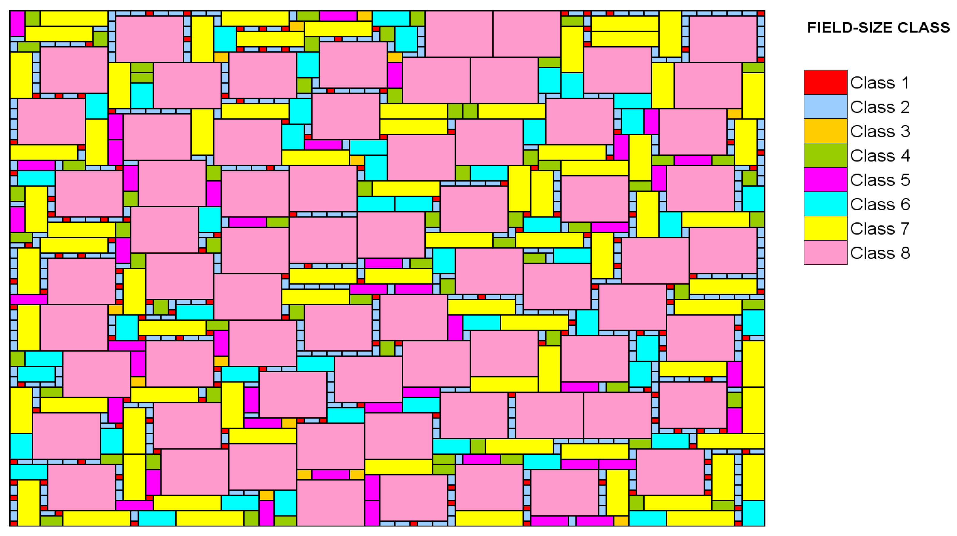
Figure 2.
Model diagram of the weed life cycle and the gene flow submodels for a depth-structured seed bank in a cereal cropping season. The state variables for the weed life cycle submodel are the seed bank, SB, the seedlings, SL, the adult plants, AD and the seed rain, SR. Other variables which take part in the gene flow submodel are seeds that are imported and exported by the harvester, IS and ES, the seeds contaminating the crop grain at the harvest timing, CG, the seeding density at the crop seeding timing, CCG, the seeds caught by seed catching, SC, and the frequency of the resistance alleles in the pollen cloud, ppo and qpo. The constant of the model are the seed interchange fraction between the three soil layers for each tillage plough, t1, t2 and t3, the structured germination fraction, g, of each cohort, c, the natural seed bank mortality fraction, m, the seedling survival fraction following the tillage operation, s, the seed bank predation fraction, d, the survival fraction following the control exerted by the herbicide application, h, the natural seedling survival fraction, v, the mutation rate, k, and the potential fecundity of an isolated plant, f.
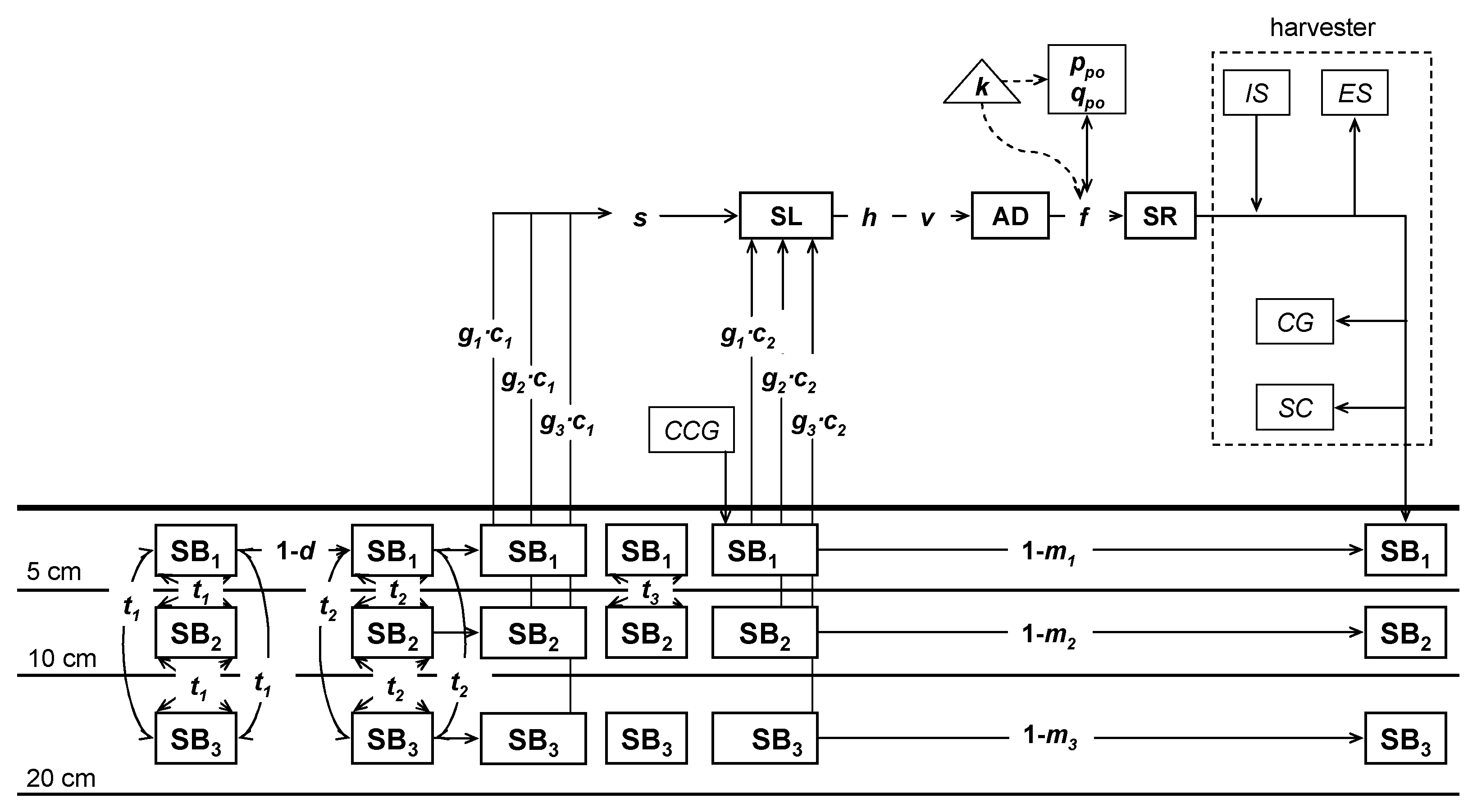
Figure 3.
Growth rate of the phenotype frequency of the herbicide-resistant L. rigidum population across the entire landscape.
Figure 3.
Growth rate of the phenotype frequency of the herbicide-resistant L. rigidum population across the entire landscape.
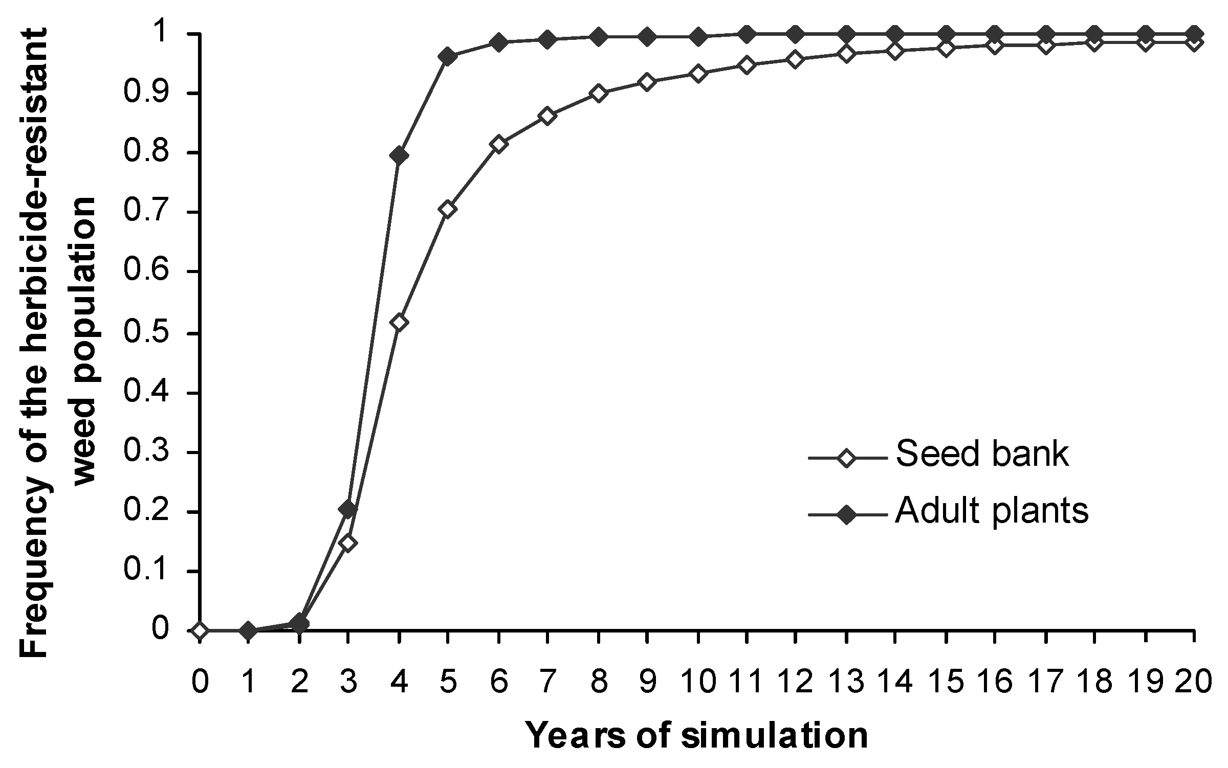
Figure 4.
Growth rate of the phenotype frequency of the herbicide-resistant L. rigidum seed bank across the entire landscape and for different cropping systems.
Figure 4.
Growth rate of the phenotype frequency of the herbicide-resistant L. rigidum seed bank across the entire landscape and for different cropping systems.
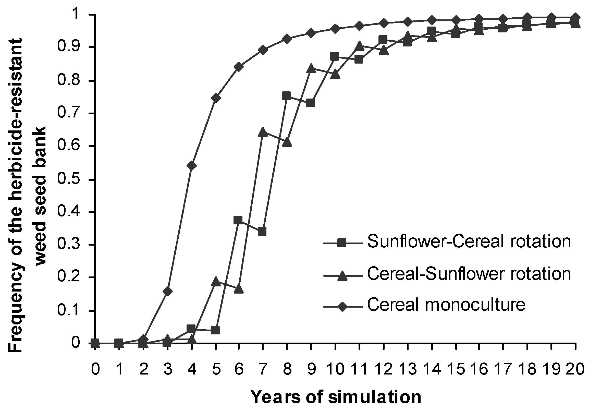
Figure 5.
Spread of the resistance over the landscape. .
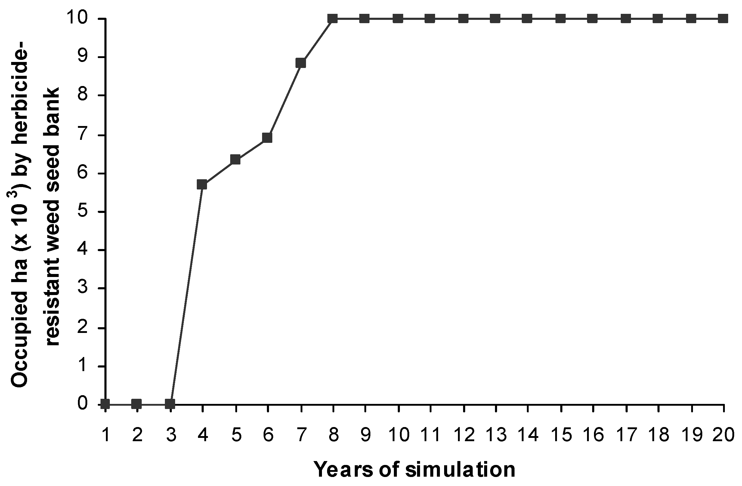
Figure 6.
Spread of the resistance over the landscape at 1, 4, 6 and 8 year time. Each level of resistance is specified in different color in the pictures. Where SBAA, SBaA and SB are the homozygous resistant, the heterozygous resistant and the total seed bank (SB= SBAA + SBaA + SBaa) respectively.
Figure 6.
Spread of the resistance over the landscape at 1, 4, 6 and 8 year time. Each level of resistance is specified in different color in the pictures. Where SBAA, SBaA and SB are the homozygous resistant, the heterozygous resistant and the total seed bank (SB= SBAA + SBaA + SBaa) respectively.
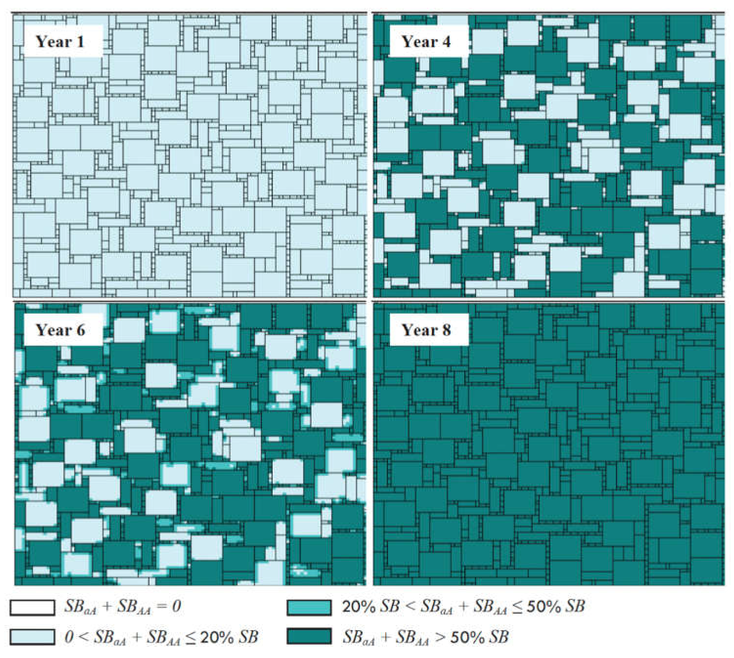
Figure 7.
Weed seed bank in the individual strategies simulated EST1 to EST5 (A) and in the combinations of all individual strategies simulated EST6 to EST16 (B) to control the herbicide resistance with respect to the reference conditions (EST0). Some strategies underlie one another in the two graphics. (Meaning of the abbreviations in Table 3).
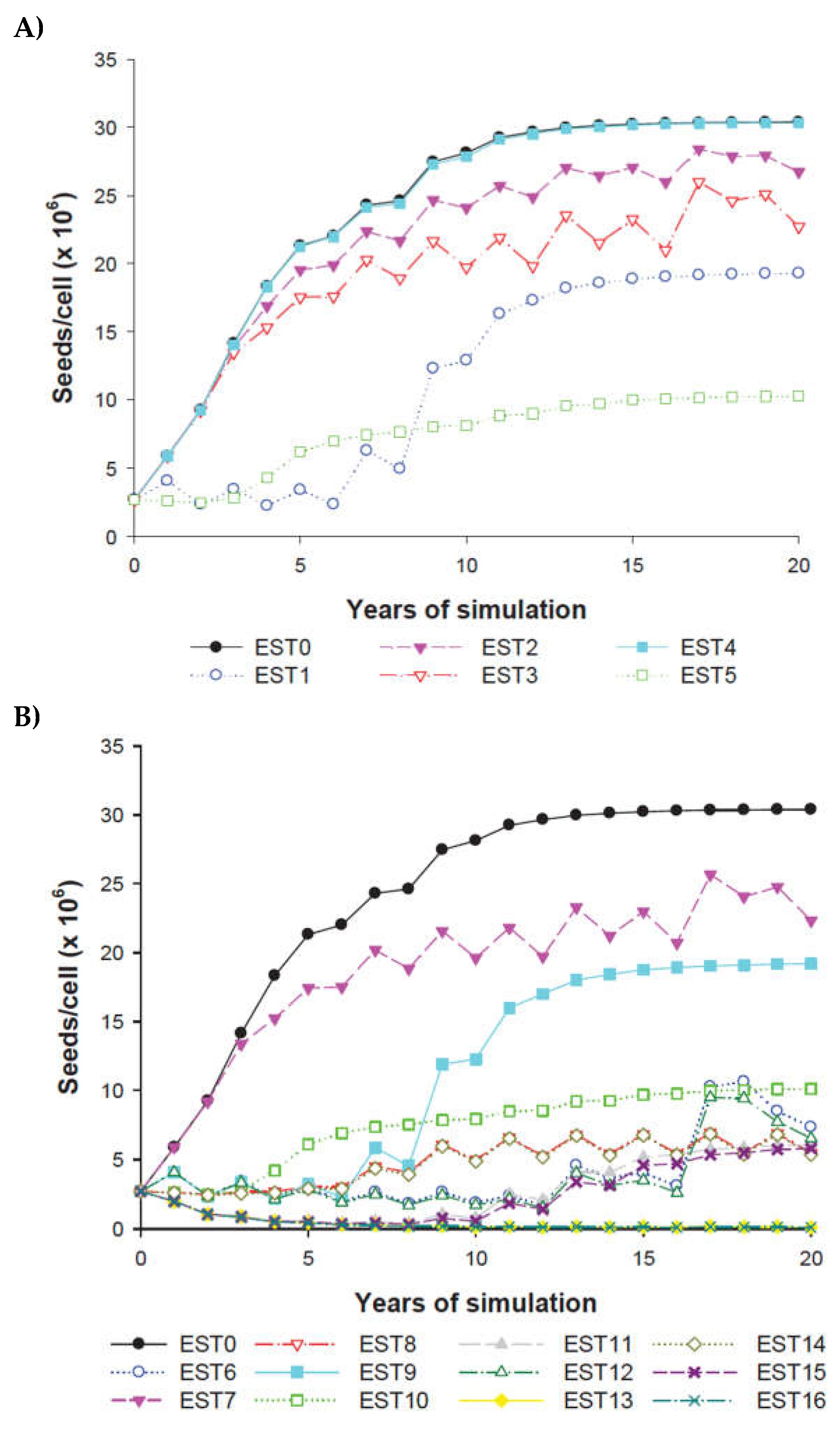
Figure 8.
The phenotype frequency of herbicide resistance in the individual strategies simulated EST1 to EST5 (A) and in the combinations of all individual strategies simulated EST6 to EST16 (B) to control the herbicide resistance with respect to the reference conditions (EST0). Some strategies underlie one another in the two graphics. (Meaning of the abbreviations in Table 3).
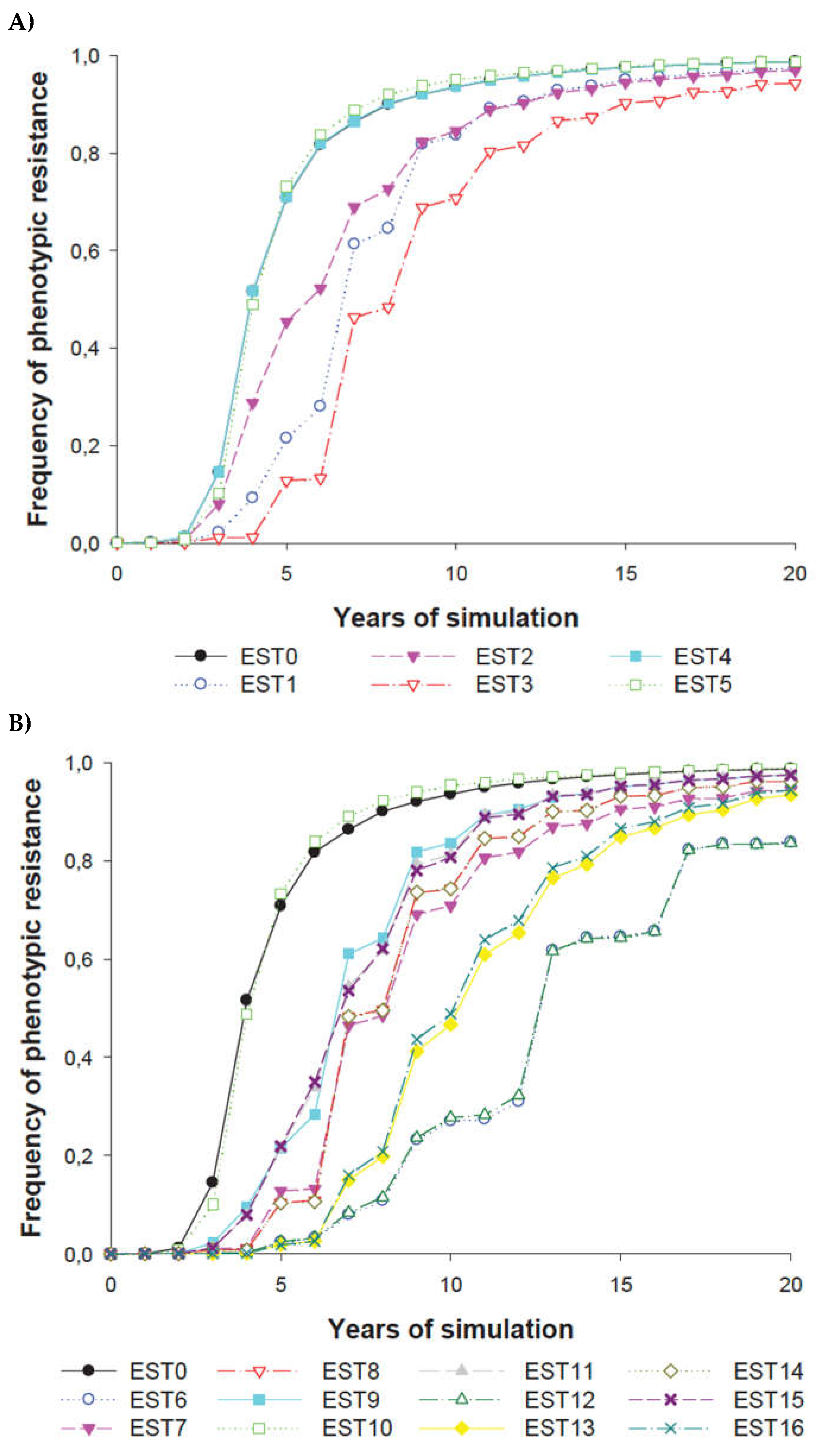
Figure 9.
The cells occupied by an herbicide-resistant population in the individual strategies simulated EST1 to EST5 (A) and in the combinations of all individual strategies simulated EST6 to EST16 (B) to control the herbicide resistance with respect to the reference conditions (EST0). Some strategies underlie one another in the two graphics. (Meaning of the abbreviations in Table 3).
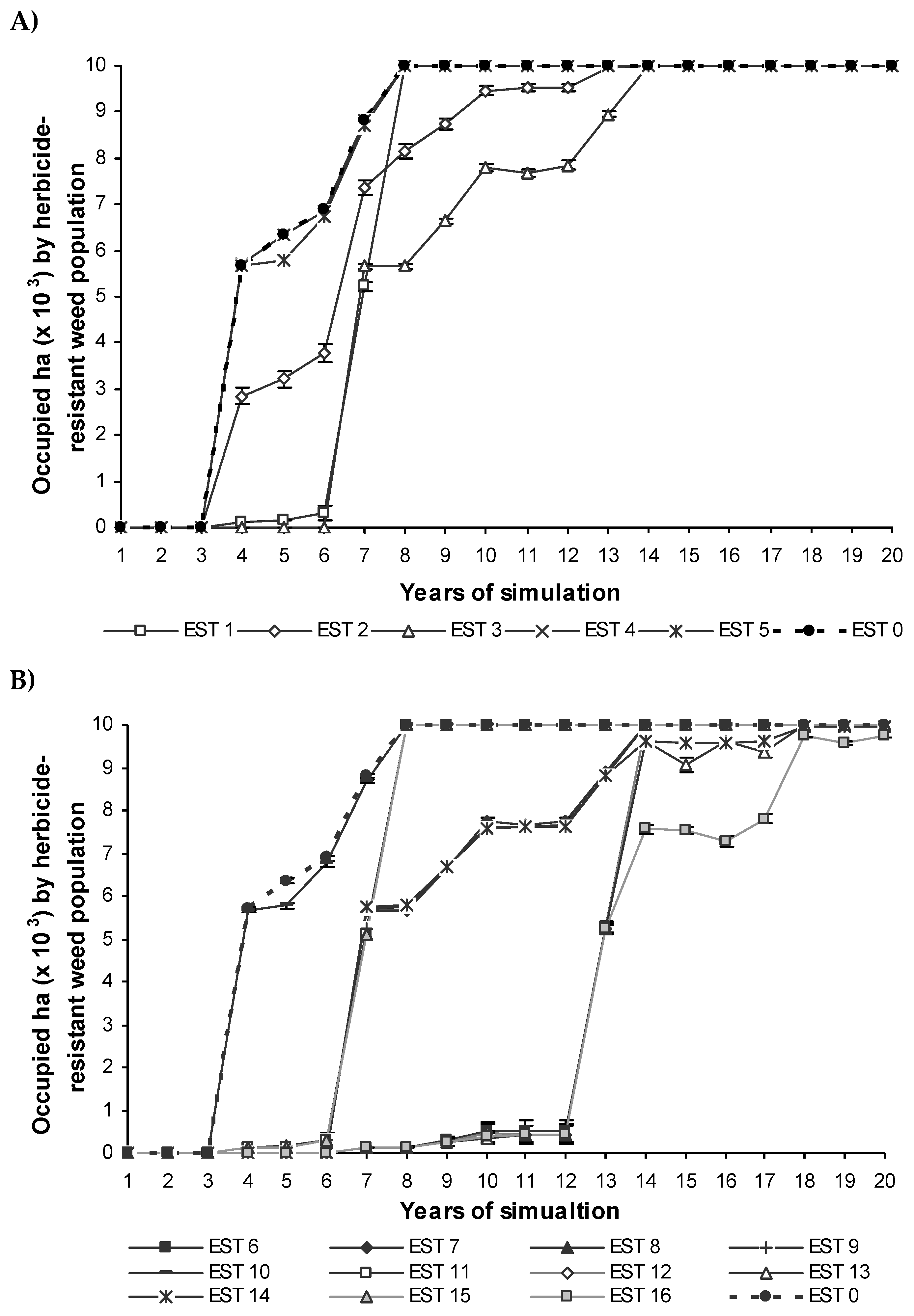
Figure 10.
Herbicide resistance spread over the landscape (A) and the distance of the infested area from the resistance focus (B) for the individual dispersal sources of gene flow (harvester, weed-contaminated crop seeding and pollen flow). Vertical bars indicate the ranges of variation.
Figure 10.
Herbicide resistance spread over the landscape (A) and the distance of the infested area from the resistance focus (B) for the individual dispersal sources of gene flow (harvester, weed-contaminated crop seeding and pollen flow). Vertical bars indicate the ranges of variation.
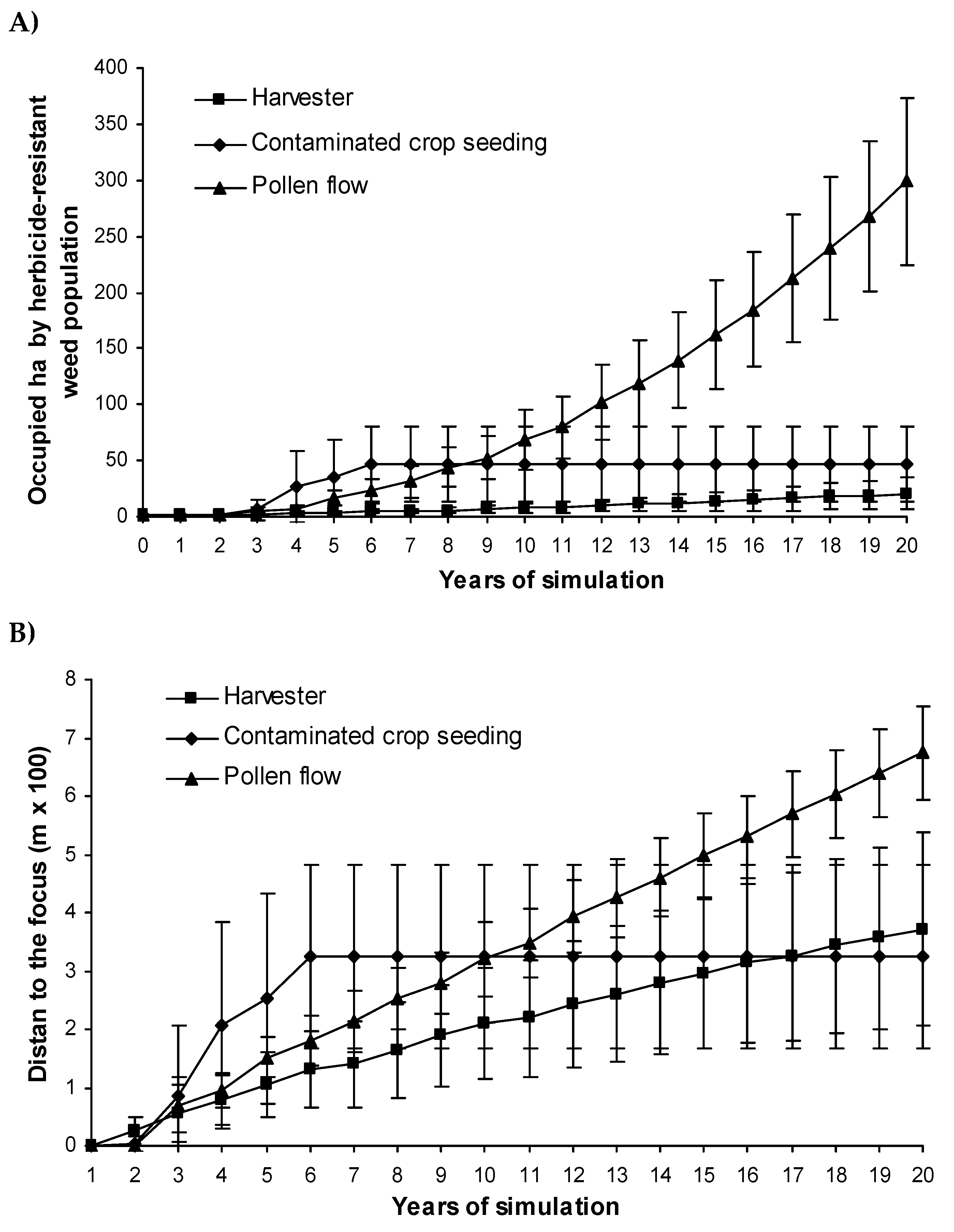
Figure 11.
The sensitivity analysis of the model for the quantitative parameters evaluated according to the conditions specified in section 1 and for two of the outputs analyzed: the years to resistance evolution across the entire landscape (A) and the years to resistance evolution in half of the landscape (B). The minimum value of the potential fecundity is no shown because the herbicide resistance did not evolve in the weed population at the landscape scale in 20-year time of simulations.
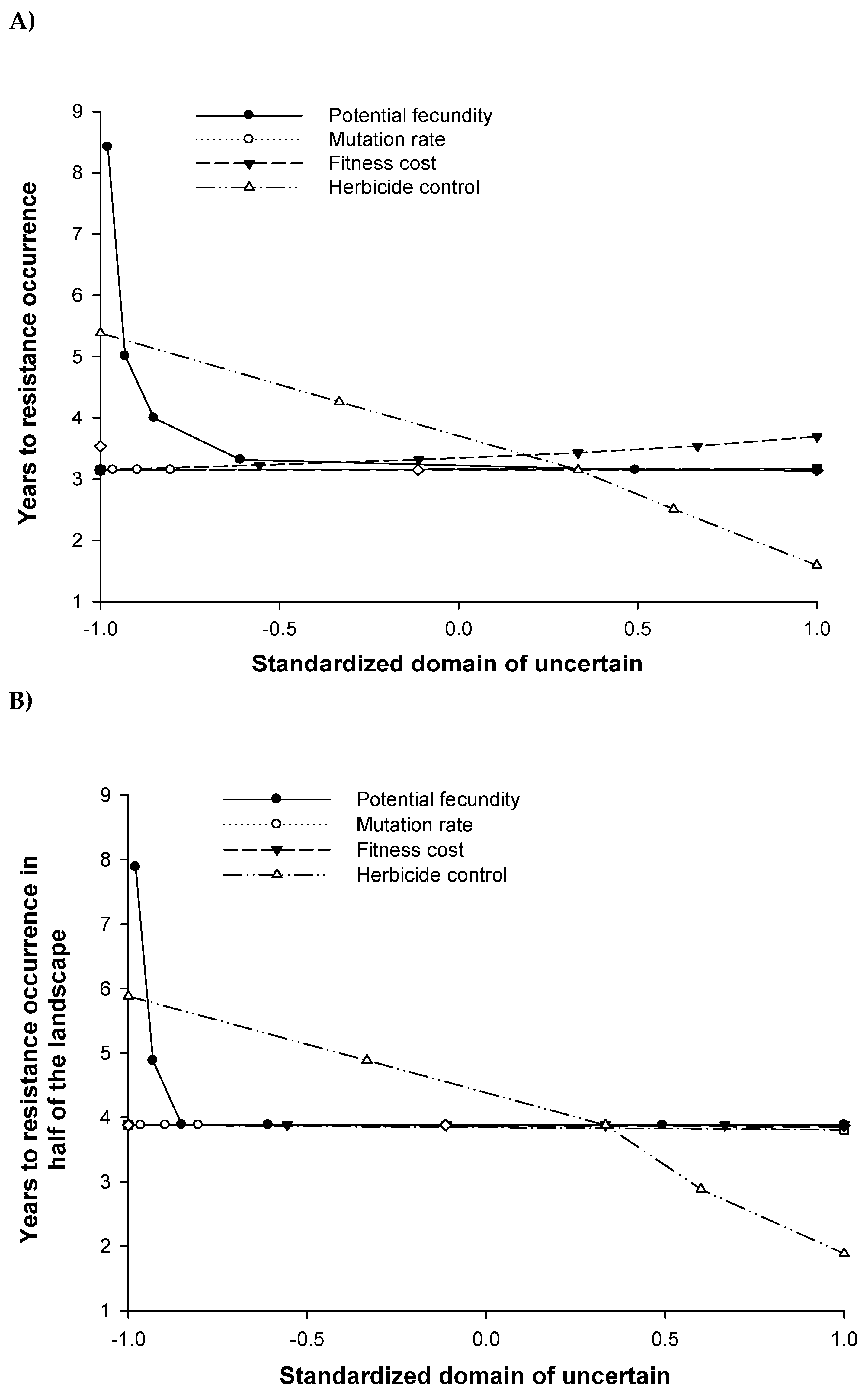
Figure 12.
The sensitivity analysis of the model for the parameters (A) and modules (B) evaluated according to the conditions specified in section 3.
Figure 12.
The sensitivity analysis of the model for the parameters (A) and modules (B) evaluated according to the conditions specified in section 3.
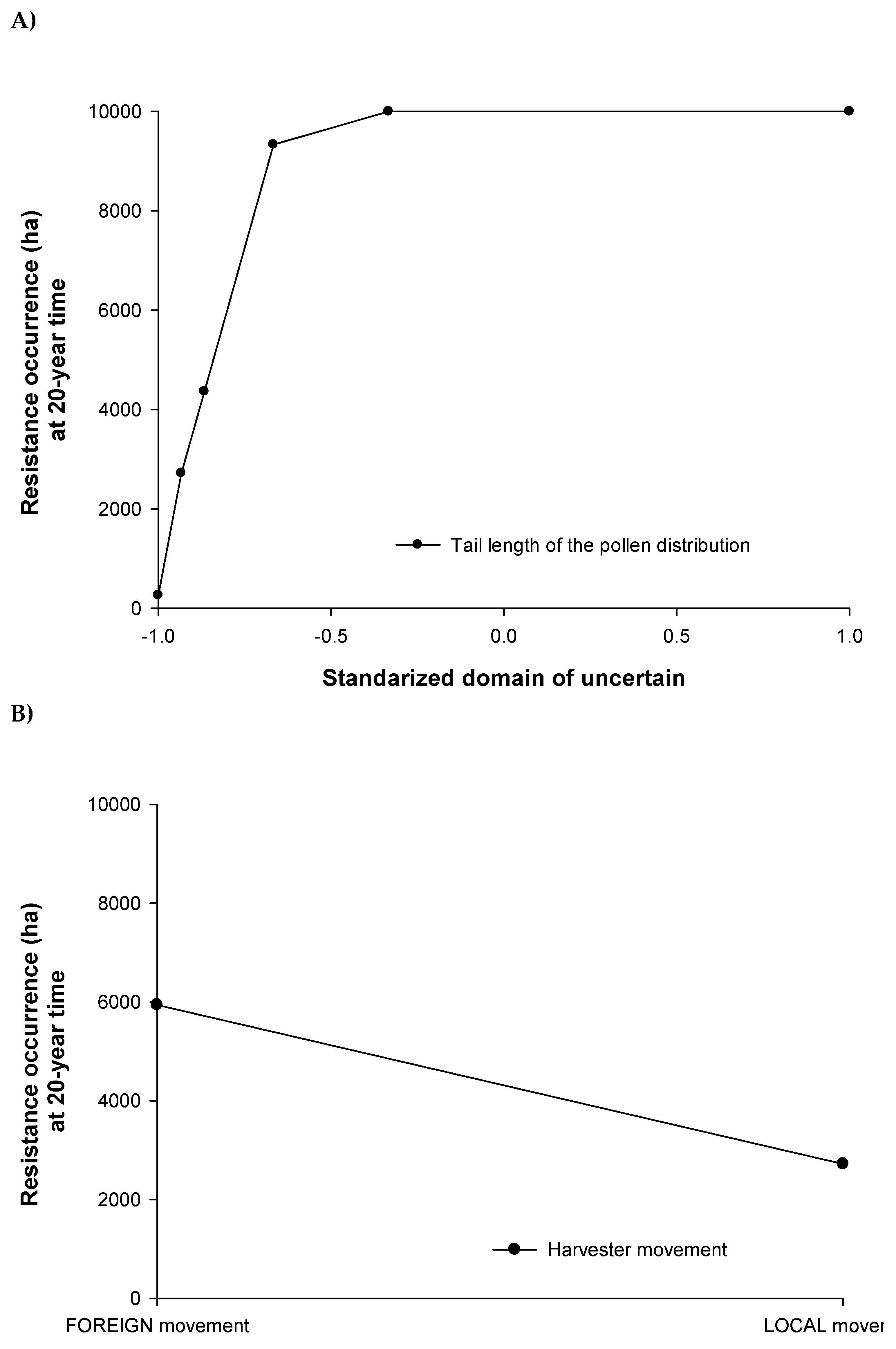
Table 1.
Field-size classes and the major crop distribution according to the Andalusian landscape [22].
Table 1.
Field-size classes and the major crop distribution according to the Andalusian landscape [22].
| Field-size class |
Unit field size (ha/field) |
Field dimension |
Number of fields |
Total field size (ha) |
Cereal crops (%) | Sunflower crops (%) |
|---|---|---|---|---|---|---|
| Class 1 | 1 | 1 x 1 | 26 | 26 | 89 | 11 |
| Class 2 | 2 | 1 x 2 | 74 | 148 | 88 | 12 |
| Class 3 | 4 | 2 x 2 | 77 | 308 | 69 | 31 |
| Class 4 | 6 | 2 x 3 | 108 | 648 | 79 | 21 |
| Class 5 | 10 | 2 x 5 | 59 | 590 | 81 | 19 |
| Class 6 | 15 | 3 x 5 | 57 | 855 | 77 | 23 |
| Class 7 | 27 | 3 x 9 | 56 | 1512 | 78 | 22 |
| Class 8 | 81 | 9 x 9 | 73 | 5913 | 77 | 23 |
Table 2.
Initial conditions and parameter values and their sources for L. rigidum growing in cereal and sunflower crops.
Table 2.
Initial conditions and parameter values and their sources for L. rigidum growing in cereal and sunflower crops.
| Description | Symbol | Cereal crop | Sunflower crop | Reference | ||||||
|---|---|---|---|---|---|---|---|---|---|---|
| Initial conditions | ||||||||||
| Initial seed bank | SBini | 2.7 · 106 seeds/ha * | 2.7 · 106 seeds/ha * | [2] | ||||||
| Initial frequency of herbicide-resistant allele | pini | 2.16 · 10-5 † | 2.16 · 10-5 † | [31] | ||||||
| Initial weed seeds in the crop seeding density for each genotype |
|
0 ‡ 0 0 |
0 ‡ 0 0 |
|||||||
| Parameters of the model | ||||||||||
| First tillage operation, t1 | t111 t112, t113 |
t121 t122 t123 |
t131 t132 t133 |
0.59 0.34 0.07 |
0.41 0.50 0.09 |
0.06 0.06 0.88 |
0.70 ¶ 0.20 0.10 |
0.15 0.53 0.32 |
0.01 0.03 0.96 |
[32] |
| Second tillage operation, t2 | t211 t212, t213 |
t221 t222 t223 |
t231 t232 t233 |
0.80 0.13 0.07 |
0.13 0.74 0.13 |
0.01 0.01 0.98 |
0.85 § 0.15 0 |
0.31 0.69 0 |
0 0.04 0.96 |
[32] |
| Thirst tillage operation, t3 | t311 t312, t313 |
t321 t322 t323 |
t331 t332 t333 |
1 ** 0 0 |
0 1 0 |
0 0 1 |
0.80 ¶ 0.13 0.07 |
0.13 0.74 0.13 |
0.01 0.01 0.98 |
[32] |
| Removal fraction by predation activity | d | 0.5 †† | 0.5 †† | [24] | ||||||
| Germination fraction Soil layer 1 Soil layer 2 Soil layer 3 |
g1 g2 g3 |
0.53 ‡‡ 0.27 0.02 |
0.53 ‡‡ 0.27 0.02 |
[33] | ||||||
| Contribution of each weed cohort to the total germination fraction Cohort 1 Cohort 2 |
c1 c2 |
0.65 ¶¶ 0.35 |
0.65 ¶¶ 0.35 |
[34] | ||||||
| Survival fraction following mechanical control | s2 s3 |
0 §§ 1 ** |
0 §§ 0 §§ |
|||||||
| Herbicide control for each genotype | haa haA hAA |
0.95 a 0 0 |
0 b 0 0 |
|||||||
| Natural seedling survival fraction | v | 0.76 | 0.76 | [35] | ||||||
| Potential seed production | f | 935 seeds/plant | 935 seeds/plant | [28] | ||||||
| Parameter of the hyperbolic model | b | 0.000034 ha c | 0.000034 ha c | [28] | ||||||
| Mortality of the seed bank Soil layer 1, 2 and 3 |
m1 = m2 = m3 |
0.30 ‡‡ |
0.30 ‡‡ |
[36] |
||||||
| Mutation rate for herbicide resistance | k | 2.7·10-8 d | 2.7·10-8 d | [37] | ||||||
| Maximum ring around focus cell which is achieved by pollen dispersal | z | 1 e | 1 e | [38] | ||||||
| Spread and weighted pollen at distance Parent cell Ring 1 |
pol0 pol1 |
1 e 0.029 |
1 e 0.029 |
[38] | ||||||
| Harvester parameters |
gat con exp |
0.91 f 0.08 f 0.02 g |
0 h 0 0 |
[39] |
||||||
* Calculated from the average L. rigidum adult plants in cereal fields of Andalusia landscape. † Averaged from the frequency of L. rigidum survivors under herbicide selection in the laboratory experiments and assuming the populations are in Hardy-Weinberg equilibrium. ‡ A crop seeding density free of weed seeds was initially considered in both crops. ¶ The one-centimeter soil layers of [39] study were aggregated according to the soil layer depths in the model. § No literature available. The plowing matrix for the scarifier was taken from the data of chisel plow. ** The tillage operation was not implemented. †† Taken from data of Lolium multiflorum and Vicia villosa seeds removed by invertebrate predators from dryland cereal fields. ‡‡ The data from the soil layer depths in the reference were aggregated according to the soil layer depths in the model. ¶¶ Averaged from the herbicide-susceptible individuals. §§ The tillage operation was supposed to eliminate all established seedlings. a Herbicide resistance was a dominant trait. Data estimated according to the L. rigidum control exerted by commercial doses of herbicides [40]. b Herbicide was not applied in the sunflower crops. c Value fitted to ha from m2 unit in the reference for L. rigidum. d Taken from the mutation rate for the primisulfuron herbicide in tobacco plants. e Calculated as the probability of a Lolium perenne pollen grain to be spread further than 80 meters. f Calculated according to the fraction of L. rigidum seeds taken from the cereal fields and the fraction of such which are incorporated to the crop grain [41]. g Calculate as the probability of the weed seeds getting into the harvester in a 100-meters trajectory would spread in the next cell [39]. h No literature availability. There is a low probability that L. rigidum seeds spread long distances from the source during sunflower harvester or contaminate the sunflower seeds due to the enormous differences in the morphology of both sunflower and L. rigidum seeds. i Calculated according to the fraction of L. rigidum seeds eliminated from the cereal grain in the cleaning process.
Table 3.
Single strategies and multiple strategies (i. e., combination of individual control strategies) simulated.
Table 3.
Single strategies and multiple strategies (i. e., combination of individual control strategies) simulated.
| Strategies | Description |
|---|---|
| EST 1 | Crop rotation in the 100% of the landscape |
| EST 2 | Rotation of herbicide modes of action in the 50% of the landscape |
| EST 3 | Rotation of herbicide modes of action in the 100% of the landscape |
| EST 4 | Sowing of certified cereal crop seed in the 100% of the landscape |
| EST 5 | Seed catcher connected to the cereal harvester |
| EST 6 | EST 1 + EST 3 |
| EST 7 | EST 3 + EST 4 |
| EST 8 | EST 3 + EST 5 |
| EST 9 | EST 1 + EST 4 |
| EST 10 | EST 4 + EST 5 |
| EST 11 | EST 1 + EST 5 |
| EST 12 | EST 1 + EST 3 + EST 4 |
| EST 13 | EST 1 + EST 3 + EST 5 |
| EST 14 | EST 3 + EST 4 + EST 5 |
| EST 15 | EST 1 + EST 4 + EST 5 |
| EST 16 | EST 1 + EST 3 + EST 4+ EST 5 |
Disclaimer/Publisher’s Note: The statements, opinions and data contained in all publications are solely those of the individual author(s) and contributor(s) and not of MDPI and/or the editor(s). MDPI and/or the editor(s) disclaim responsibility for any injury to people or property resulting from any ideas, methods, instructions or products referred to in the content. |
© 2024 by the authors. Licensee MDPI, Basel, Switzerland. This article is an open access article distributed under the terms and conditions of the Creative Commons Attribution (CC BY) license (http://creativecommons.org/licenses/by/4.0/).
Copyright: This open access article is published under a Creative Commons CC BY 4.0 license, which permit the free download, distribution, and reuse, provided that the author and preprint are cited in any reuse.


