1. Introduction
1.1. The Growing Demand for Precision Agriculture
In the face of a burgeoning global population and the escalating pressures of climate change, ensuring food security and maximizing agricultural productivity have become paramount concerns [
1,
2,
3]. To achieve these goals, farmers and agricultural stakeholders are increasingly turning to precision agriculture, a data-driven approach that optimizes crop management practices based on real-time information and analysis. Accurate prediction of crop yield is a fundamental aspect of precision agriculture, as it enables informed decision-making regarding resource allocation, harvest timing, and supply chain management [
4,
5].
1.2. The Importance of Accurate Napa Cabbage Fresh Weight Prediction in Modern Agriculture
Napa cabbage (Brassica rapa L. ssp. pekinensis), a staple crop in East Asia, plays a vital role in regional diets and economies. However, its production faces numerous challenges, including susceptibility to price fluctuations due to its short storage life and sensitivity to environmental factors such as abnormal weather patterns and fluctuating cultivation areas [
6,
7,
8]. Accurate and timely prediction of Napa cabbage yield is crucial for efficient resource allocation, effective supply chain management, and price stabilization. The accurate prediction of Napa cabbage fresh weight is crucial for mitigating these challenges and ensuring a stable supply of this essential crop.
The ability to accurately predict Napa cabbage fresh weight before harvest offers numerous benefits to various stakeholders in the agricultural sector:
Farmers: Precise yield prediction empowers farmers to make informed decisions regarding harvest timing, ensuring optimal quality and maximizing market value while minimizing post-harvest losses [
9,
10]. Additionally, it enables farmers to tailor crop management strategies, such as irrigation and fertilization, based on real-time insights into crop growth and development, thereby improving resource use efficiency and reducing environmental impact [
11,
12,
13].
Agribusinesses: Reliable yield forecasts facilitate better supply chain management, ensuring adequate inventory levels, reducing food waste, and mitigating price volatility [
14]. This leads to increased profitability and a more stable market for both producers and consumers.
Policymakers: Accurate yield predictions inform national-level decision-making, enabling governments to develop effective agricultural policies, anticipate potential shortages, and implement measures to ensure food security [
15,
16]. This is particularly crucial in the context of climate change, where unpredictable weather patterns can significantly impact crop yields.
Traditional methods for estimating Napa cabbage fresh weight, relying on manual sampling and visual inspection, are labor-intensive, time-consuming, and prone to human error [
17]. Moreover, these methods lack the spatial and temporal resolution required for precise field-scale assessment, hindering the ability to detect subtle variations in crop growth and development. While remote sensing technologies, such as satellite imagery, offer a broader perspective, they may not be sufficient for capturing the nuanced variations in Napa cabbage growth and development [
18,
19]
1.3. The Potential of UAVs and AI in Agriculture
The integration of unmanned aerial vehicles (UAVs) with advanced sensors and artificial intelligence (AI) algorithms offers a transformative solution to these limitations. UAVs, or drones, equipped with high-resolution RGB [
20], multispectral [
21], and thermal infrared (TIR) sensors [
22], can efficiently collect detailed data on crop health, vigor, and yield potential at a fine spatial and temporal scale [
23]. This data, combined with the computational power of AI, enables the development of sophisticated models for predicting crop yield and other essential parameters.
The integration of AI algorithms with UAV-based remote sensing data has further enhanced the capabilities of yield prediction models. Numerous studies have demonstrated the potential of UAV-based remote sensing and AI in various agricultural applications, including crop classification [
24,
25], monitoring of growth [
26], nutritional status [
27,
28], yield prediction [
29,
30,
31], and disease detection [
32]. AI algorithms, particularly deep learning techniques, excel at processing large volumes of data and identifying complex patterns and relationships that may not be apparent through traditional statistical methods. AI algorithms, particularly deep learning techniques, have shown exceptional promise in extracting meaningful features from UAV imagery and accurately predicting crop yield, even in complex and dynamic environments [
33]. To develop models that accurately predict Napa cabbage fresh weight based on various factors, including vegetation indices, crop height, canopy cover, and water stress indicators are necessary.
1.4. Objectives and Contributions of This Study
This study aims to address the current limitations in Napa cabbage fresh weight prediction by developing a comprehensive AI-powered model that leverages UAV-based multi-sensor data. Specifically, we aim to: Develop a robust and accurate model: Integrate RGB, multispectral, and TIR imagery with AI algorithms (deep neural network; DNN, support vector machine; SVM, and random forest; RF) to predict Napa cabbage fresh weight. Identify the optimal growth stage: Determine the most informative period during the Napa cabbage growth cycle for accurate fresh weight prediction. Evaluate model performance: Assess the accuracy, generalizability, and robustness of the developed model using various evaluation metrics. Analyze spatial variability: Investigate the influence of soil type and irrigation on Napa cabbage fresh weight and its prediction. Identify challenges and future directions: Discuss the limitations of the current approach and propose potential areas for future research.
2. Materials
2.1. Study Area and Experimental Plot Design
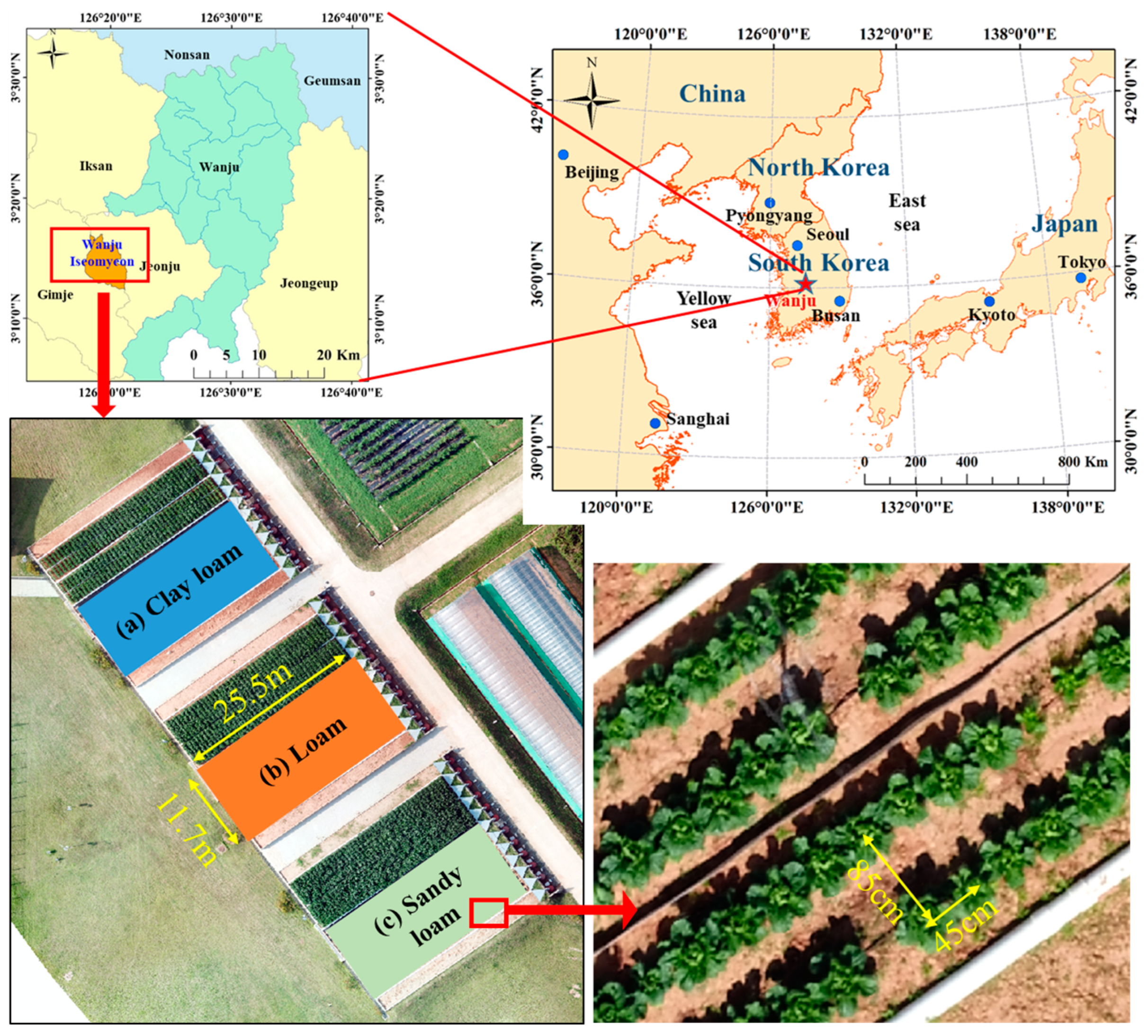
This study was conducted in 2020 at the Napa cabbage cultivation test field of the National Institute of Agricultural Sciences, located in Iseo-myeon, Wanju-gun, Jeollabuk-do, Rep. of Korea (127°02′49.65″E, 35°49′28.52″N) (
Figure 1).
The experimental plots were designed on a slope of approximately 7 degrees to simulate the typical terrain of Napa cabbage cultivation areas in Korea. The test field comprised three plots, each with an area of 290 m², and distinct soil conditions: clay loam, loam, and sandy loam. Each plot measured 25.5 m × 11.7 m. The study focused on fall Napa cabbage ('Cheongomabi' variety), planted in late August and harvested in early November, with a planting distance of 45 cm × 85 cm. Standard cultivation methods were employed throughout the study period.
In 2020, a non-watering treatment was implemented for the Napa cabbage grown in the loam plot, relying solely on rainfall for water supply. The other two plots (clay loam and sandy loam) were maintained under standard irrigation practices.
2.2. Unmanned Aerial Vehicles and Sensors
A rotary-wing UAV, the DJI Inspire 2, was utilized for image acquisition throughout the fall Napa cabbage growth cycle. The Inspire 2 was equipped with three distinct sensors: 1) an RGB camera (Zenmuse X5s, DJI) with a 20-megapixel resolution to capture standard red, green, and blue (RGB) light wavelengths; 2) a multispectral sensor (RedEdge-M, Micasense) designed to capture light wavelengths beyond the visible spectrum, providing valuable insights into plant health and vegetation indices; and 3) a TIR sensor (Vue Pro R, FLIR) capable of measuring the thermal radiation emitted by objects, enabling assessment of plant temperature and water stress. This integrated multi-sensor approach facilitated the collection of comprehensive data encompassing the Napa cabbage's morphological, physiological, and thermal characteristics throughout the growing season.
2.3. Fall Napa Cabbage Growth Cycle and Data Collection Timeline
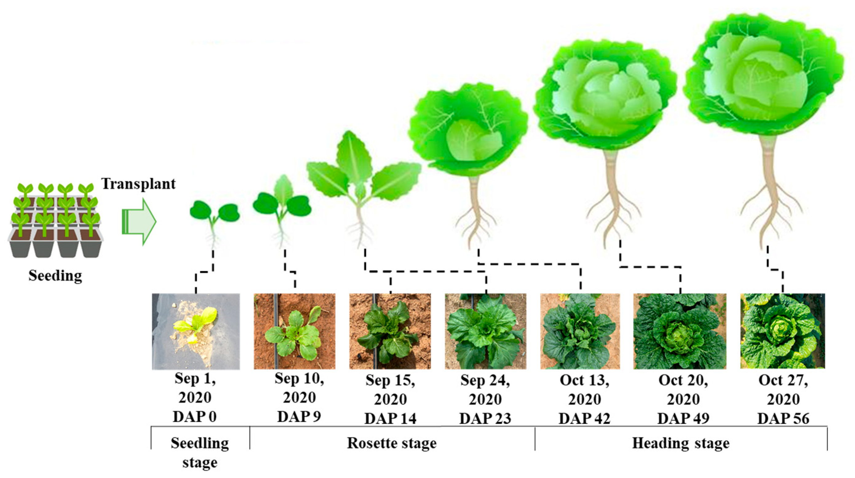
Fall Napa cabbage (cv. 'Cheongomabi') typically follows a 70-day growth cycle, starting from late August planting to early November harvest. In this study, seedlings were sown in pots and transplanted to the field after 15-20 days. The growth cycle is characterized by three distinct stages (
Figure 2):
Seedling Stage (DAP 0-7): This initial stage encompasses root establishment and early vegetative growth post-transplanting.
Rosette Stage (DAP 9-42): The longest growth phase, marked by a rapid increase in leaf number and expansion of leaf area.
Heading Stage (DAP 49-56): The final stage, characterized by the cessation of leaf growth and the formation of a compact, spherical head as the inner leaves mature.
To monitor the entire growth cycle for the fresh weight prediction model, UAV imaging and field surveys were conducted at 7~10day intervals from late August to early November, capturing data across all growth stages, including the pre-planting period.
3. Materials
3.1. Study Flow Chart
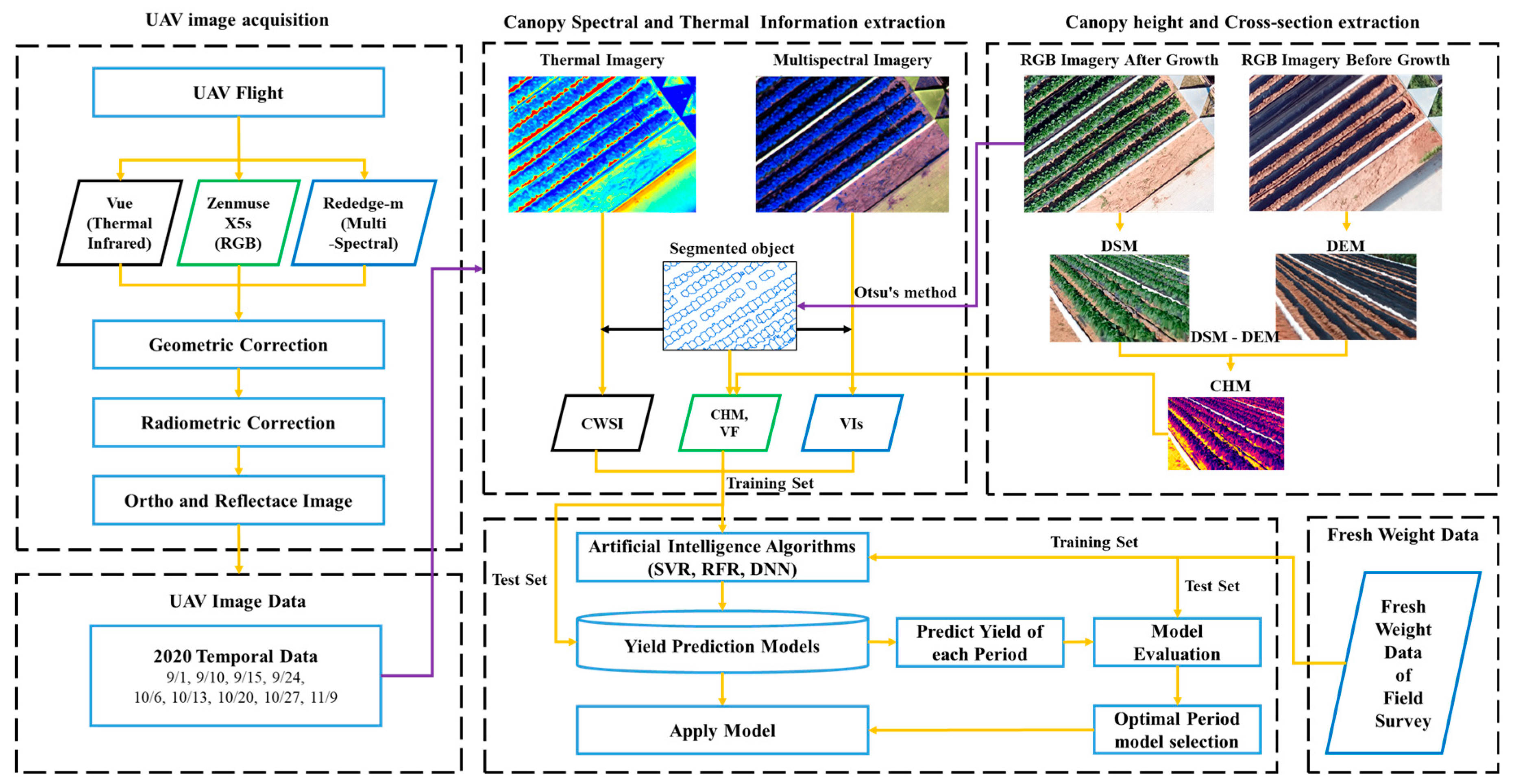
The overall study process, as depicted in
Figure 3, followed a systematic sequence: data collection, image preprocessing, data preprocessing, AI model construction and evaluation, and ultimately, fresh weight prediction for each fall Napa cabbage plant. UAV imagery and corresponding field data were collected in 2020. The acquired images underwent preprocessing, including geometric and radiometric corrections, to ensure accuracy and consistency. Utilizing the 2020 time-series data, further preprocessing was conducted to extract relevant features and normalize the data for subsequent analysis. AI models were then constructed and evaluated for each data collection date, employing a range of algorithms to identify the optimal model for fresh weight prediction. The selection of the final model involved assessing its performance at different growth stages and determining the most effective algorithm.
The detailed methodologies for each stage of the fresh weight study, including image preprocessing, data preprocessing, AI model construction and evaluation, and fresh weight calculation, are presented in subsequent sections as outlined in
Figure 3.
3.2. UAV Image Acquisition and Preprocessing
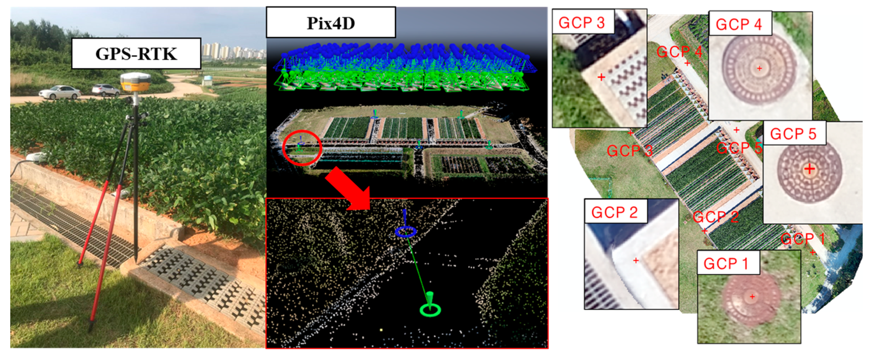
UAV imagery was captured at a 30 m altitude using a DJI Inspire 2 UAV equipped with alternating combinations of RGB and multispectral (MSP) sensors, as well as RGB and TIR sensors. The acquired MSP imagery underwent geometric and radiometric correction using Pix4D mapper software. Geometric correction was achieved by incorporating the measured coordinates of five ground control points (GCPs), selected on unchanging objects within the field (e.g., manholes), into the preprocessing workflow (
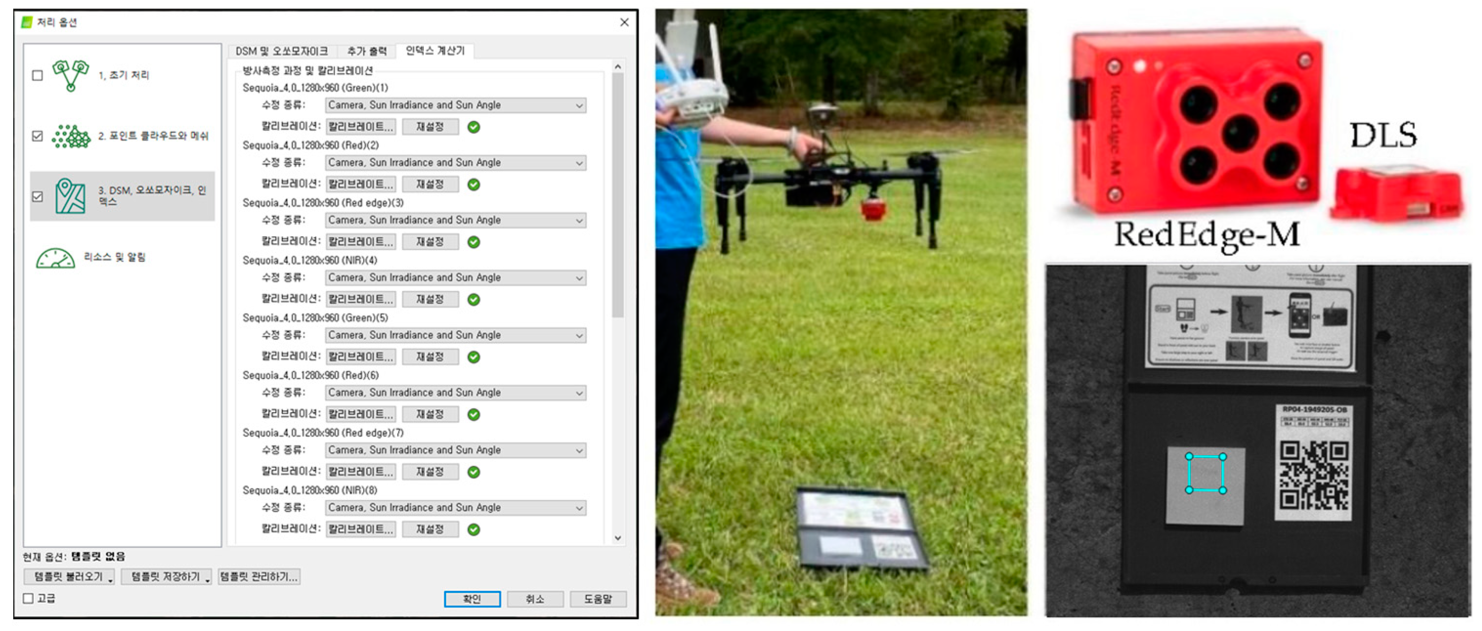
Figure 4). Radiometric correction was performed using both a reflectance correction panel image taken before flight and real-time light quantity data obtained from a Downwelling Light Sensor (DLS) (
Figure 5).
Table 1 details the UAV image acquisition schedule for the 2020 fall Napa cabbage growing season, aligned with key growth stages. On-site image capture and field surveys were conducted at 7 to 10-day intervals from August to November, resulting in nine image acquisitions across the season. This comprehensive dataset facilitated detailed monitoring of Napa cabbage growth dynamics and enabled the extraction of various vegetation indices for subsequent analysis.
3.3. Field Survey
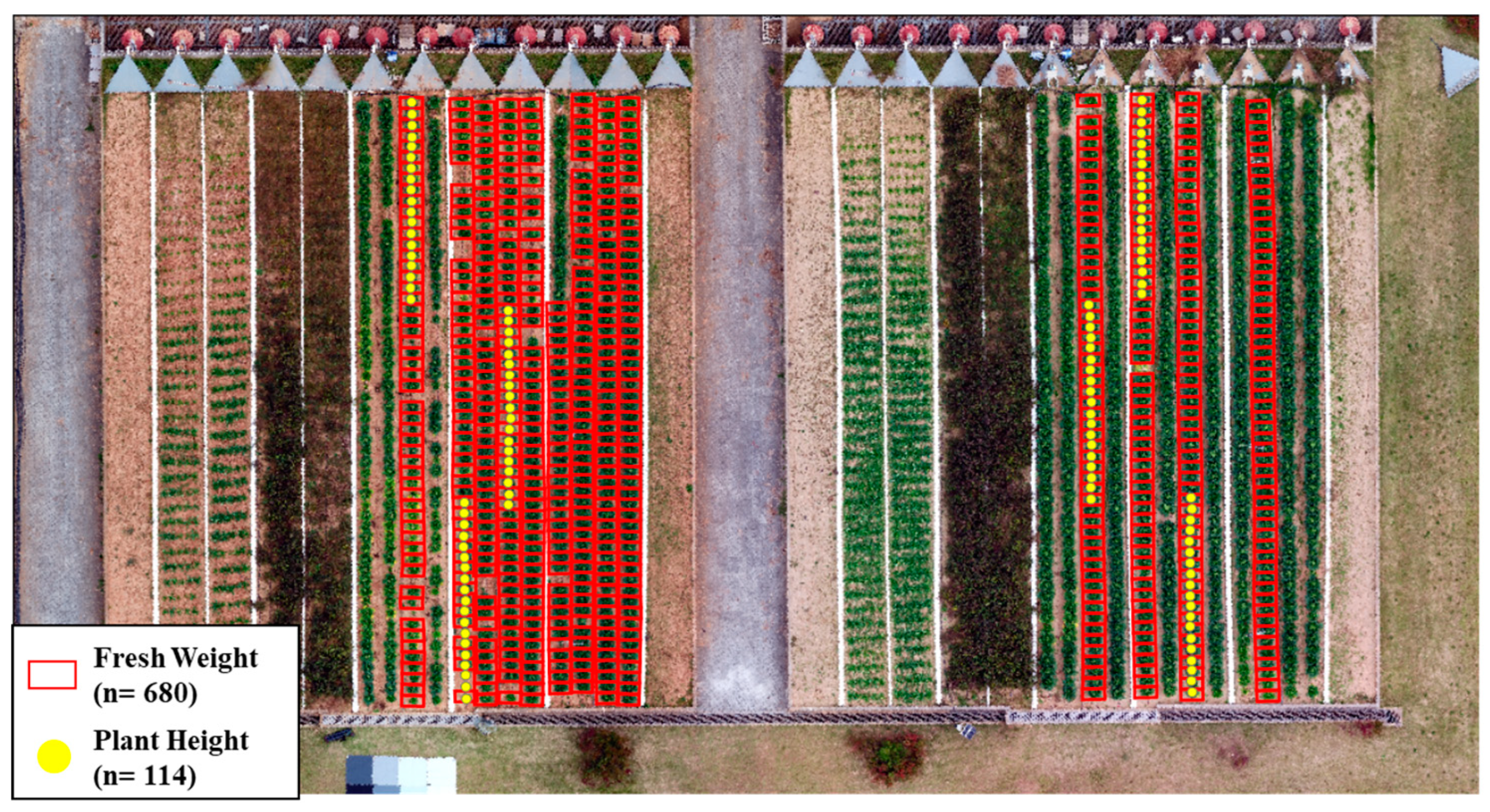
Field surveys were conducted to measure plant height and fresh weight, two key indicators of Napa cabbage growth. Plant height was determined by measuring the distance from the ground to the highest leaf at each survey time point. A subset of 114 Napa cabbages was selected for draft measurements to compare with model predictions. To maintain consistency, both UAV image acquisition and Napa cabbage draft surveys were conducted on the same day. The specific locations of these 114 sampled Napa cabbages are indicated by yellow dots in
Figure 6.
On November 9, 2020, the final harvest date, the fresh weight of 680 Napa cabbages was measured. For these Napa cabbages, both location information and fresh weight were recorded, forming a comprehensive dataset. Additionally, the fresh weight of 625 Napa cabbages not selected as samples was measured randomly, albeit without location information. The spatial distribution of the 680 georeferenced Napa cabbage samples is illustrated by red boxes in
Figure 6.
The data collected through these field surveys served as ground truth for training and evaluating the AI models developed to predict Napa cabbage fresh weight. The subsequent sections detail the analysis and results derived from these models.
3.4. Individual Napa Cabbage Object Segmentation
To analyze individual Napa cabbage plants, it is necessary to segment the cabbage objects. This study utilized Excess Green (ExG) index, Otsu's thresholding method, and grid generation techniques to achieve this segmentation.
3.4.1. Excess Green (ExG) Image Extraction
The ExG vegetation index [
34], calculated as ExG = 2G - R - B (where R, G, and B represent reflectance values in the red, green, and blue bands, respectively), was utilized in this study to enhance the contrast between vegetation and background elements in RGB images captured by the Zenmuse X5s camera mounted on the Inspire 2 UAV. This index leverages the principle that healthy vegetation reflects more green light than red or blue light, resulting in positive ExG values for green vegetation and negative values for non-green areas like soil or water. Higher positive ExG values generally correlate with healthier vegetation.
In this study, a custom Python script was employed to extract ExG images from the RGB imagery. These ExG images served as valuable inputs for generating additional vegetation indices, which were subsequently used as features in the AI models for fresh weight prediction. The utilization of ExG images proved advantageous due to their simple calculation, relative insensitivity to varying illumination and atmospheric conditions, ability to differentiate vegetation types based on spectral reflectance, and proven effectiveness in various agricultural applications such as crop monitoring, yield prediction, and weed detection. By providing a clear distinction between Napa cabbage plants and the background soil, ExG enhanced the models' ability to focus on relevant features, leading to more accurate and precise fresh weight predictions.
3.4.2. Otsu's Method for Image Segmentation
Otsu's method, a widely used, non-parametric, and unsupervised image segmentation algorithm [
35], was employed to distinguish foreground (Napa cabbage plants) from background (soil) in grayscale images. This method maximizes the inter-class variance (
σ²_B), a measure of dissimilarity between the two classes, to determine an optimal threshold.
The inter-class variance at a given threshold t is calculated as:
where,
ω_0(t) and
ω_1(t) represent the weights (proportional to the number of pixels) of the background and foreground classes, respectively, at threshold t.
σ²_0(t) and
σ²_1(t) represent the variances of the background and foreground classes, respectively, at threshold
t.
The optimal threshold (
t*) is determined by iterating over all possible threshold values and selecting the one that maximizes the inter-class variance, as shown in Equation (2):
In this study, Otsu's method was applied to grayscale versions of the ExG images derived from UAV captured RGB imagery to segment individual Napa cabbage plants from the background soil. The resulting binary images facilitated the accurate calculation of vegetation indices and other features, which were essential inputs for the AI models used to predict Napa cabbage fresh weight. This automatic segmentation process proved crucial for precise feature extraction, ultimately contributing to the successful prediction of Napa cabbage fresh weight.
3.4.3. Process of Individual Napa Cabbage Object Segmentation
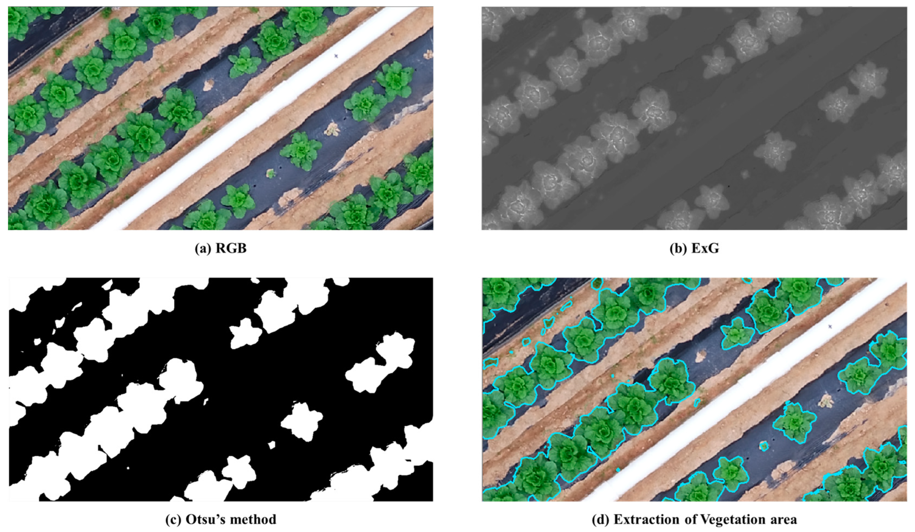
Individual Napa cabbage objects were segmented from UAV imagery using a multi-step process (
Figure 7).
First, RGB images were converted to ExG indices to enhance the contrast between vegetation and background (
Figure 7b). Otsu's thresholding method was then applied to the ExG images, generating binary masks that differentiated vegetation from non-vegetation areas (
Figure 7c). These masks were subsequently vectorized, retaining only the vegetation regions, effectively outlining the Napa cabbage plants (
Figure 7d).
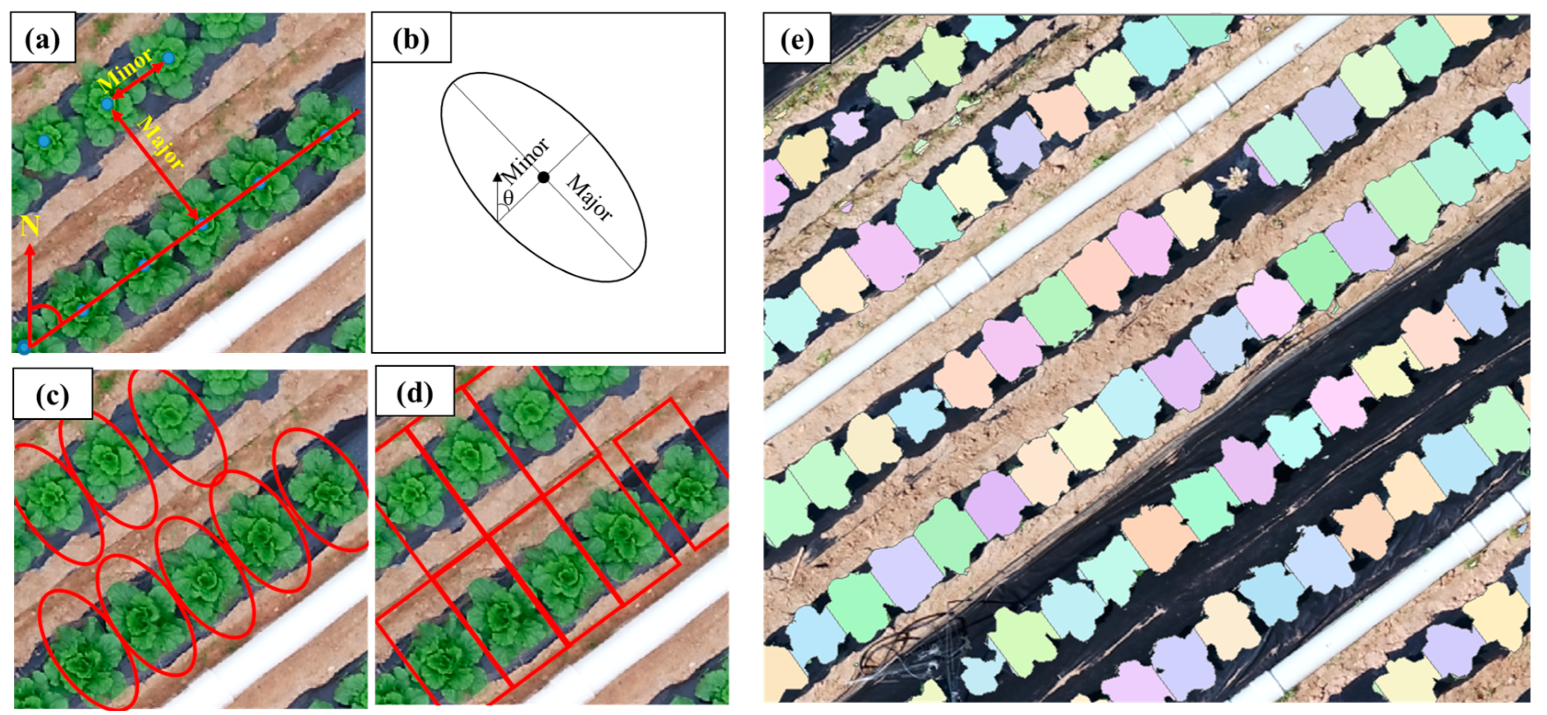
However, due to the overlapping nature of Napa cabbage plants during the rosette growth stage, the initial segmentation often grouped multiple plants as a single object. To address this, a grid-based approach was implemented in ArcGIS Pro (Esri, USA) to delineate individual plants (
Figure 8). First, the center point of each Napa cabbage object was digitized (
Figure 8a). An ellipse was then generated around each point, with major and minor axes corresponding to the valley and planting spacing, respectively, and the angle θ representing the row orientation relative to true north (
Figure 8b). These ellipses were adjusted to match the actual location of each Napa cabbage plant within the row, resulting in distorted ellipses aligned with the true north direction (
Figure 8c). The ellipses were then converted into inscribed rectangular grids (
Figure 8d), which were used to separate the overlapping Napa cabbage vector data, enabling the final segmentation of individual Napa cabbage objects (
Figure 8e).
The segmented object areas were used to extract individual growth information for each Napa cabbage plant, such as vegetation indices, crop height, and canopy cover. This information served as crucial input features for the subsequent fresh weight prediction models.
3.5. Definition of Independent Variables for AI Models
The independent variables for the AI algorithms predicting Napa cabbage fresh weight were derived from a multi-sensor approach, incorporating RGB, multispectral (MSP), and TIR imagery.
3.5.1. RGB-Based Independent Variables
Two variables representing the physical characteristics of Napa cabbage were selected from the RGB imagery.
Vegetation Fraction (VF): The ratio of the area occupied by each Napa cabbage plant (
Figure 8e) to the grid area corresponding to the plant (
Figure 8d), calculated as:
Crop Height Model (CHM): The height of each Napa cabbage plant was estimated using the difference between the Digital Surface Model (DSM) at each growth stage and the DSM before planting, leveraging the Structure from Motion (SfM) algorithm [
36]:
3.5.2. Multispectral Sensor-Based Independent Variables
Eight vegetation indices (VIs) known to correlate with leaf chlorophyll content (LCC), a crucial indicator of crop nitrogen status and yield, were selected based on preliminary experiments [
28] and derived from the multispectral (MSP) imagery. These indices, detailed in
Table 2, were chosen for their established relationships with chlorophyll content and their potential to provide valuable insights into cabbage growth and development.
3.5.3. Thermal Infrared Sensor-Based Independent Variable
The Crop Water Stress Index (CWSI), a measure of plant water stress, was selected as the TIR-based variable. CWSI was calculated using the formula proposed by Jones [
37], which utilizes only UAV-based TIR images:
Where, T is the temperature of individual pixels in the TIR image, Tc is the lowest temperature within the vegetation area, Th is the highest temperature within the vegetation area.
To ensure accurate CWSI calculation, only vegetation pixel temperatures were utilized, as determined using vector data delineating Napa cabbage areas.
For each of the 680 sampled Napa cabbage individuals, the average value of each independent variable within the plant's designated grid area was used as the input for the AI models. This multi-sensor approach aimed to capture the diverse aspects of Napa cabbage growth and physiology, thereby enhancing the predictive power of the fresh weight models.
3.6. Construction of Datasets and AI Models
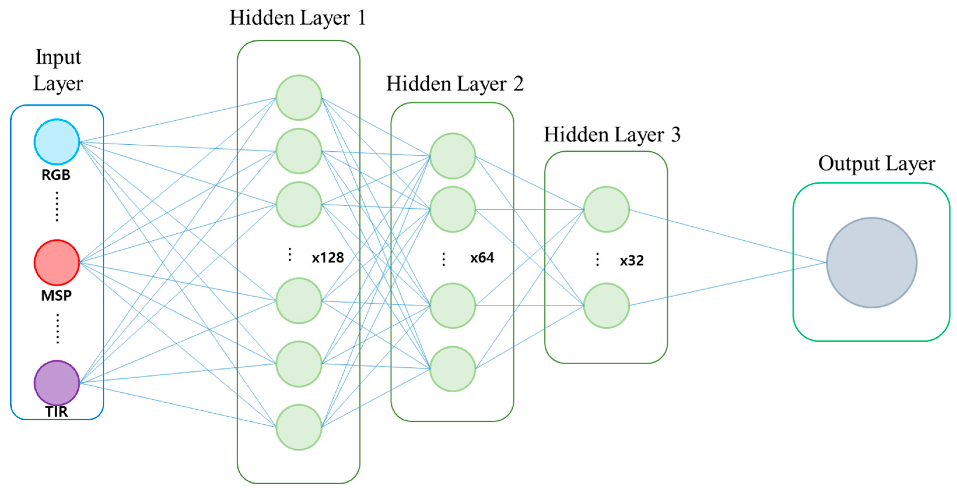
The collected dataset, comprising 680 data points, was partitioned into training (70%, 476 points) and testing (30%, 204 points) sets for hyperparameter tuning, learning, validation, and testing of the AI algorithms. This study employed three algorithms for predicting Napa cabbage fresh weight: DNN, SVM, and RF. The DNN model, analogous to the artificial neural network (ANN) algorithm, was structured with an input layer incorporating 11 independent variables (defined in
Section 3.5), followed by three hidden layers with 128, 64, and 32 nodes, respectively (
Figure 9). The output layer yielded the predicted Napa cabbage fresh weight. The ReLU activation function, chosen for its computational efficiency and ability to mitigate the vanishing gradient problem, was employed for nonlinear modeling. Optimization of the loss function was achieved using the Adam optimizer. To identify the optimal prediction time, seven DNN models were created, each trained on data from a specific period between September 10 and October 27, 2020, and their predictive accuracy was compared.
For performance comparison, SVM and RF models were also constructed. The SVM algorithm utilized the radial basis function (RBF) kernel, with hyperparameters C and gamma optimized [
45]. For the RF algorithm, the 'mtry' hyperparameter (number of variables randomly sampled as candidates at each split) was tuned [
46]. Model validation was rigorously performed using 5-fold cross-validation on 70% of the training data, repeated five times to ensure robustness and assess generalization capability.
3.7. Accuracy Evaluation
The accuracy of Napa cabbage fresh weight prediction was assessed using two metrics: the coefficient of determination (R²) and the root mean square error (RMSE). R² quantifies the proportion of variance in the observed fresh weights explained by the model, while RMSE measures the average magnitude of the prediction errors. These metrics were calculated using the following formulas;
where,
SSE (Sum of Squared Errors) is the sum of the squared differences between the observed values (
) and the predicted values (
)
, SST (Total Sum of Squares) is the sum of the squared differences between the observed values (
) and the mean of the observed values (
ȳ),
n is the total number of samples.
R² represents the proportion of the variance in the dependent variable (Napa cabbage fresh weight) that is predictable from the independent variables (the features extracted from the UAV imagery). A value of R² close to 1 indicates a good fit of the model, while a value close to 0 indicates a poor fit. The RMSE is a measure of the average magnitude of the errors in a set of predictions. RMSE quantifies the average deviation between the predicted and actual fresh weights of cabbages. A lower RMSE value indicates better predictive accuracy, as the predicted values are closer to the observed values.
4. Results
4.1. Model Accuracy Evaluation by Survey Period
The performance of three AI models (DNN, SVM, and RF) for predicting Napa cabbage fresh weight was evaluated using multi-sensor fusion data acquired from UAV flights on seven dates between September 10 and October 27, 2020 (
Table 3).
The DNN model consistently outperformed the SVM and RF models across all survey dates for both training and test datasets, as evidenced by consistently higher R² values and lower RMSE values (
Figure 10 and
Figure 11). Notably, the DNN model achieved the highest accuracy (R² = 0.82, RMSE = 0.47 kg) on October 13 (DAP 42), coinciding with the mid-rosette growth stage. The RF model, on the other hand, exhibited the lowest performance, particularly on the test dataset, suggesting potential overfitting.
The overall model performance, as indicated by R², generally improved as the Napa cabbage growth progressed. The lowest R² values were observed in the early growth stages (DAP 9-14), followed by a gradual increase and a sharp rise on October 6 (DAP 35). This trend suggests that the predictive ability of the models, especially the DNN, improved as the Napa cabbage plants matured and developed distinct morphological features.
The consistent R² values for the DNN model between training and test datasets highlight its robustness and generalizability. In contrast, the lower R² values of SVM and RF, particularly in the test dataset, indicate potential overfitting to the training data. The RMSE values further substantiate the DNN model's superior performance, consistently exhibiting the lowest prediction errors across all survey dates.
The observed superiority of the DNN model can be attributed to its deep, layered architecture, which is more adept at capturing the complex, non-linear relationships between Napa cabbage fresh weight and the multi-sensor features extracted from UAV imagery. The model's ability to learn and represent these intricate relationships contributes to its higher predictive accuracy, especially as the Napa cabbage plants mature and exhibit more distinct features during the mid-to-late rosette stage.
4.2. Model Overfitting Analysis
To assess the generalization ability of the three AI models (DNN, SVM, and RF), an overfitting analysis was conducted by comparing the performance metrics (R² and RMSE) on the training and test datasets (
Figure 12). Greater discrepancies between the metrics for the two datasets indicate a higher degree of overfitting, where the model performs well on training data but poorly on unseen data.
The DNN model exhibited exceptional stability across all growth stages (DAP 9-56), with minimal variation in both R² and RMSE differences between the training and test datasets. This suggests that the DNN model generalized well to unseen data, avoiding overfitting.
Conversely, the RF model exhibited the most significant fluctuations in R² and RMSE differences, particularly in the later growth stages (DAP 35-56), indicating a higher degree of overfitting. The SVM model showed moderate overfitting, with differences generally falling between those of the DNN and RF models.
Quantitatively, the DNN model's minimal overfitting was evident in the small discrepancies between training and test metrics: R² differences ranged from 0.013 to 0.028, and RMSE differences from 0.025 to 0.054 kg. The SVM model showed slightly larger differences, with R² ranging from 0.017 to 0.049 and RMSE from 0.033 to 0.094 kg. The RF model, however, exhibited the most pronounced overfitting, with R² differences ranging from 0.065 to 0.148 and RMSE differences from 0.125 to 0.285 kg.
Overall, the analysis indicates that the DNN model is the most robust and least prone to overfitting among the three models tested, making it the most suitable choice for predicting Napa cabbage fresh weight. These findings underscore the importance of model selection and validation in ensuring the generalizability and robustness of fresh weight predictions in agricultural applications.
4.3. Fresh Weight Prediction Performance of DNN, SVM, and RF Models
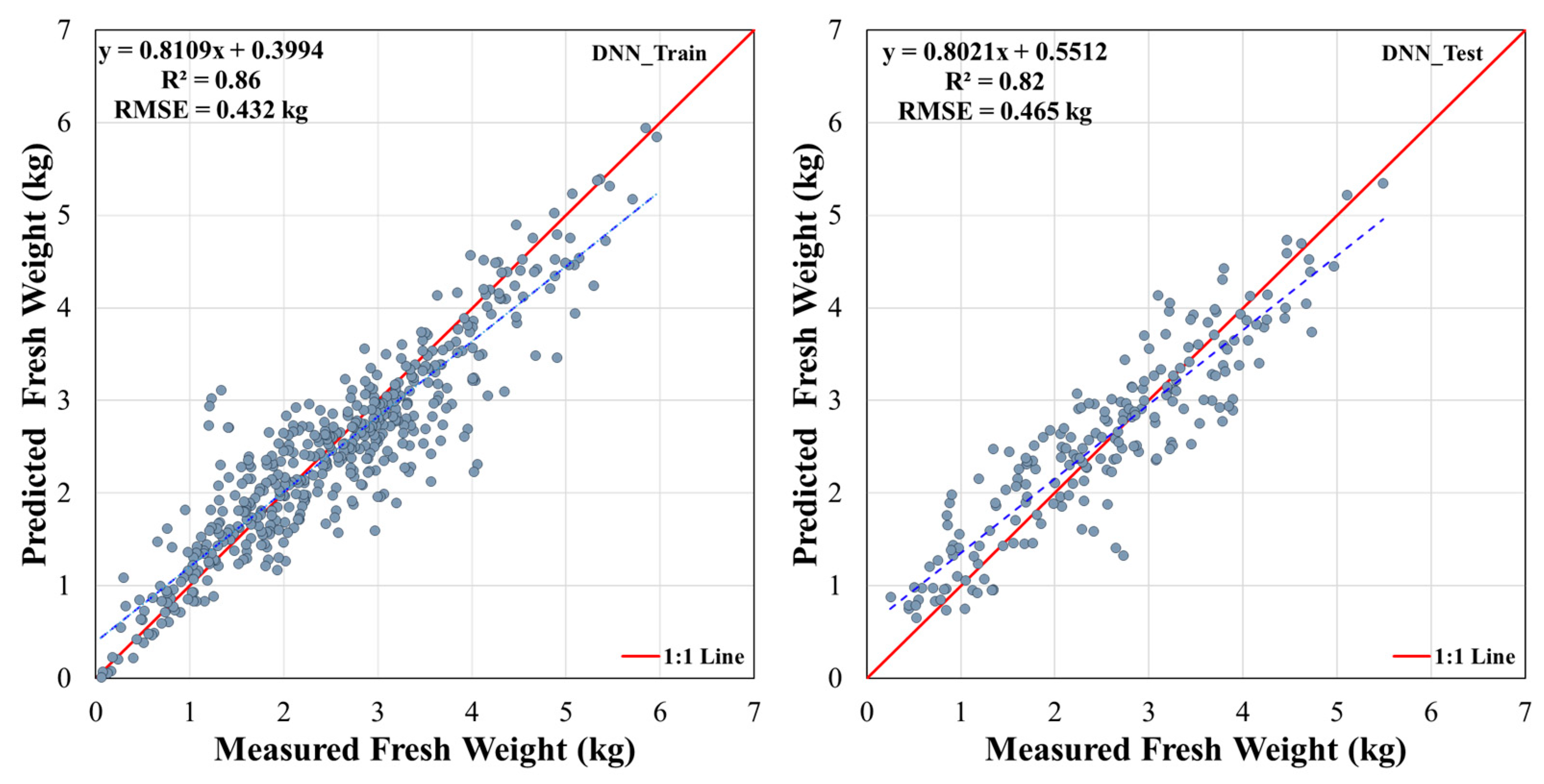
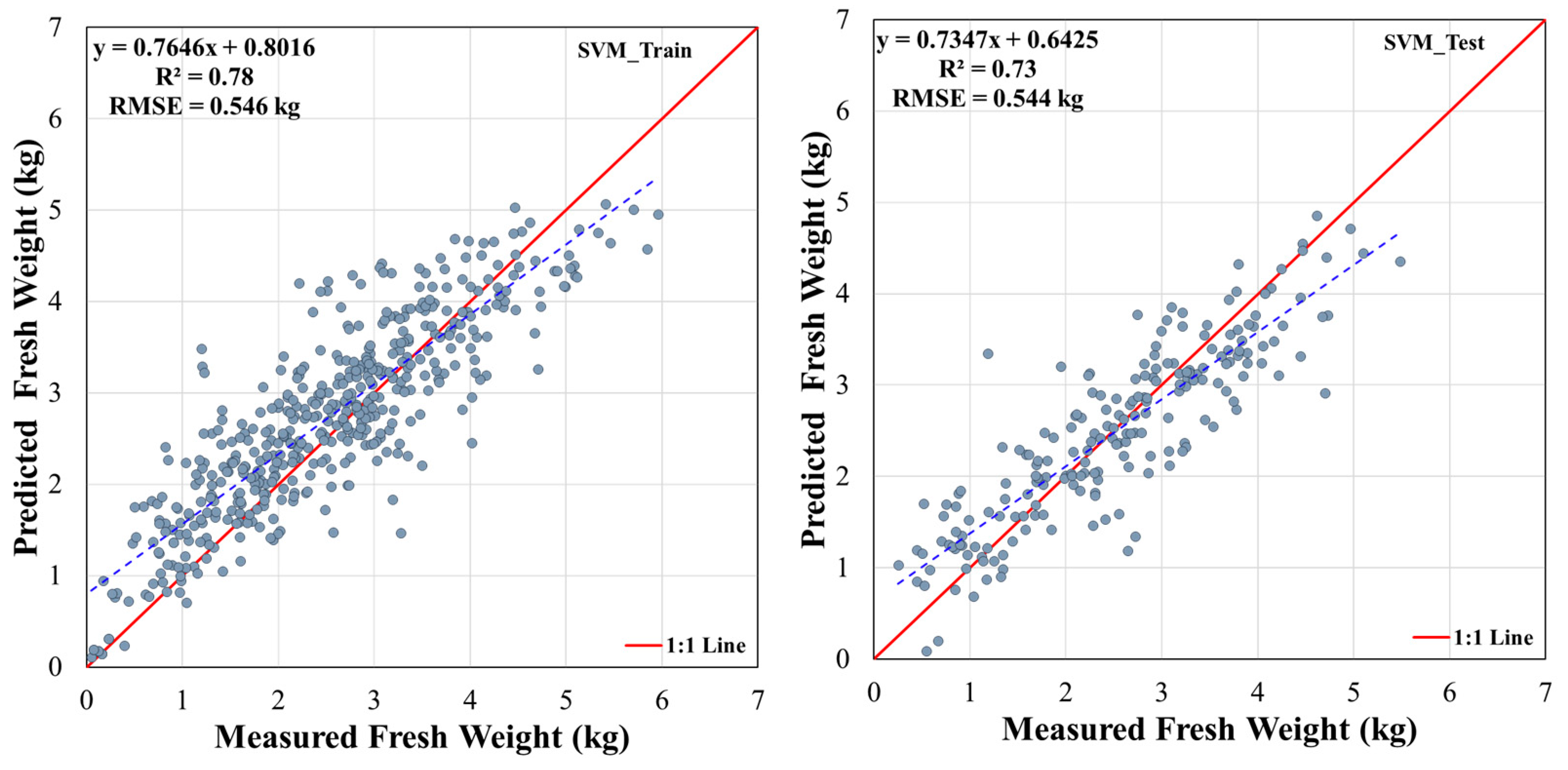
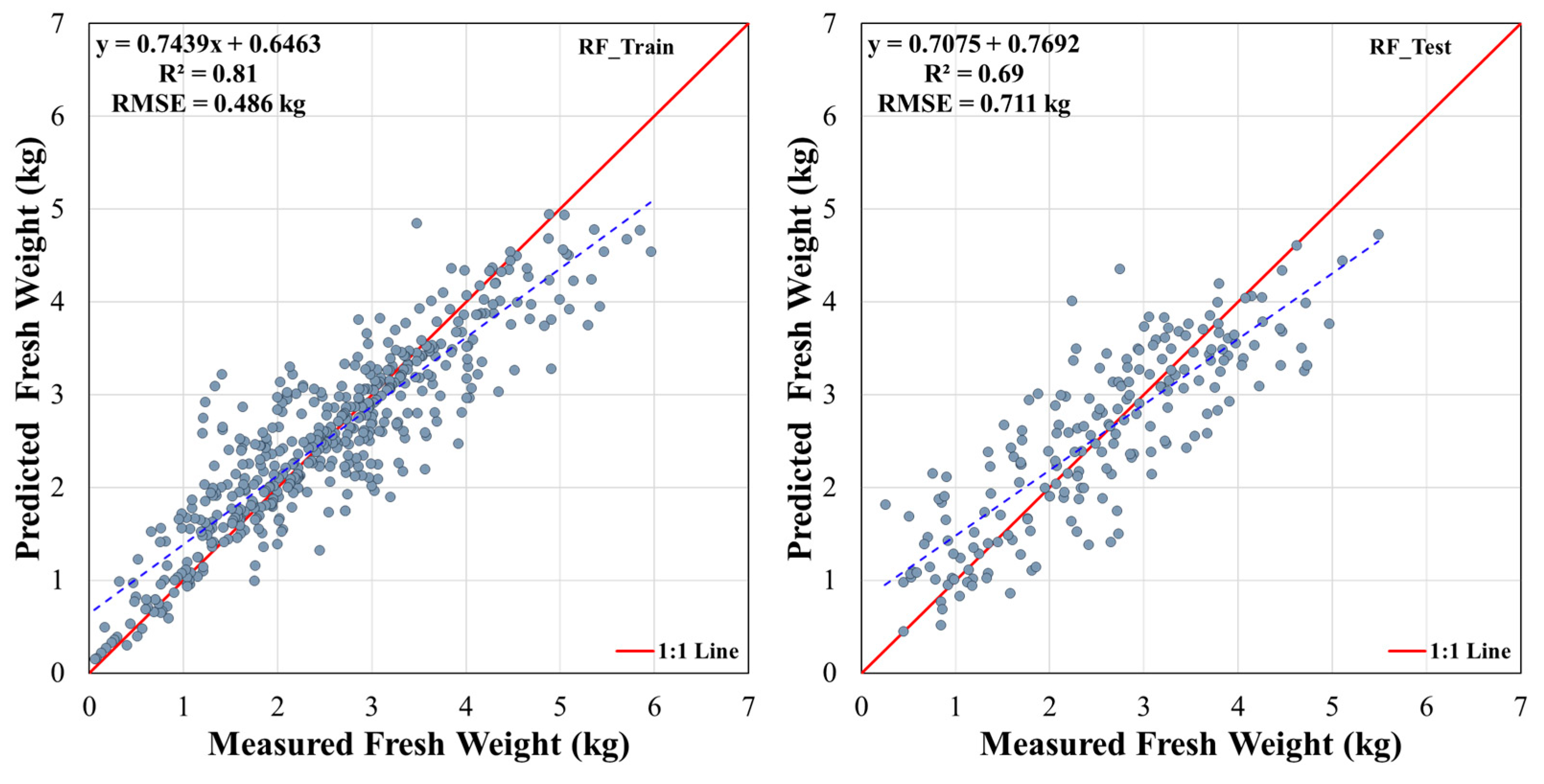
Figure 13,
Figure 14 and
Figure 15 present scatter plots comparing the predicted and measured fresh weights of individual Napa cabbage heads for the DNN, SVM, and RF models, respectively. These plots include the 1:1 line (red), regression lines (blue) with their equations, coefficients of determination (R²), and root mean square errors (RMSE).
The DNN model (
Figure 13) consistently outperformed the SVM and RF models, demonstrating the highest accuracy and generalizability. This is evidenced by the consistently high R² values (0.86 for training and 0.82 for testing) and low RMSE values (0.432 kg for training and 0.465 kg for testing) across both datasets. The close alignment of the regression lines with the 1:1 line further indicates a strong positive correlation between predicted and measured fresh weights, suggesting minimal overfitting in the DNN model.
The SVM model (
Figure 14) showed good predictive performance on the training dataset (R² = 0.78, RMSE = 0.546 kg), comparable to the DNN model. However, there was a slight decrease in accuracy and evidence of minor overfitting on the test dataset (R² = 0.73, RMSE = 0.544 kg). Despite this minor discrepancy, the SVM model still maintains a good correlation between actual and predicted fresh weights.
The RF model (
Figure 15) exhibited the lowest performance among the three models. While it showed a good correlation on the training dataset (R² = 0.81, RMSE = 0.486 kg), its accuracy significantly decreased on the test dataset (R² = 0.69, RMSE = 0.711 kg), indicating a more substantial degree of overfitting. This suggests that the RF model may not generalize well to unseen data and is less suitable for predicting Napa cabbage fresh weight in this context.
In summary, the DNN model proved to be the most accurate and robust model for predicting Napa cabbage fresh weight, followed by the SVM model with slightly lower accuracy and minor overfitting. The RF model, while performing well on the training data, exhibited the highest degree of overfitting and the lowest overall accuracy.
4.4. Bias Analysis for Overall and Fresh Weight Sections of DNN, SVM, and RF Models
Table 4 presents a fresh weight bias analysis for the DNN, SVM, and RF models, comparing their predicted values to measured values for both overall Napa cabbage weight and individual weight sections (head, stem, inner leaves, outer leaves, and total leaves). A negative bias indicates that the model overestimates the fresh weight, while a positive bias indicates underestimation.
The DNN model demonstrates the highest accuracy in predicting total Napa cabbage fresh weight, exhibiting the lowest overall bias (0.008 kg). This model tends to overestimate the fresh weight for Napa cabbages weighing less than 2 kg and underestimate it for Napa cabbages exceeding 2 kg. Conversely, the RF and SVM models show a general trend of overestimating fresh weight for Napa cabbages under 3 kg and underestimating for those over 3 kg, with overall biases of 0.031 kg and 0.041 kg, respectively.
Across individual weight sections, the DNN model consistently outperforms the other two models, demonstrating the lowest bias values for most sections. The only exception is the leaf section, where the SVM model shows a marginally lower bias (0.004 kg) compared to the DNN model (0.003 kg). However, the RF model consistently exhibits the highest bias across all weight sections, indicating its lower accuracy in predicting individual component weights.
The bias analysis further reveals the following model-specific patterns:
DNN: The highest bias (underestimation of 0.365 kg) is observed in the 4-5 kg range.
RF: The highest bias (underestimation of 0.541 kg) occurs for Napa cabbages exceeding 5 kg.
SVM: Similar to the RF model, the highest bias (underestimation of 0.88 kg) is also observed in the >5 kg range.
These findings underscore the importance of considering model-specific biases and the weight range of the Napa cabbages when selecting the most appropriate model for fresh weight prediction. The DNN model is generally the most accurate, but the SVM model may be slightly more suitable for predicting leaf weight. Furthermore, the RF model may require further refinement to improve its predictive accuracy, especially for heavier Napa cabbages.
4.5. Spatial Analysis of Measured and Predicted Napa Napa cabbage Fresh Weight Using the DNN Model
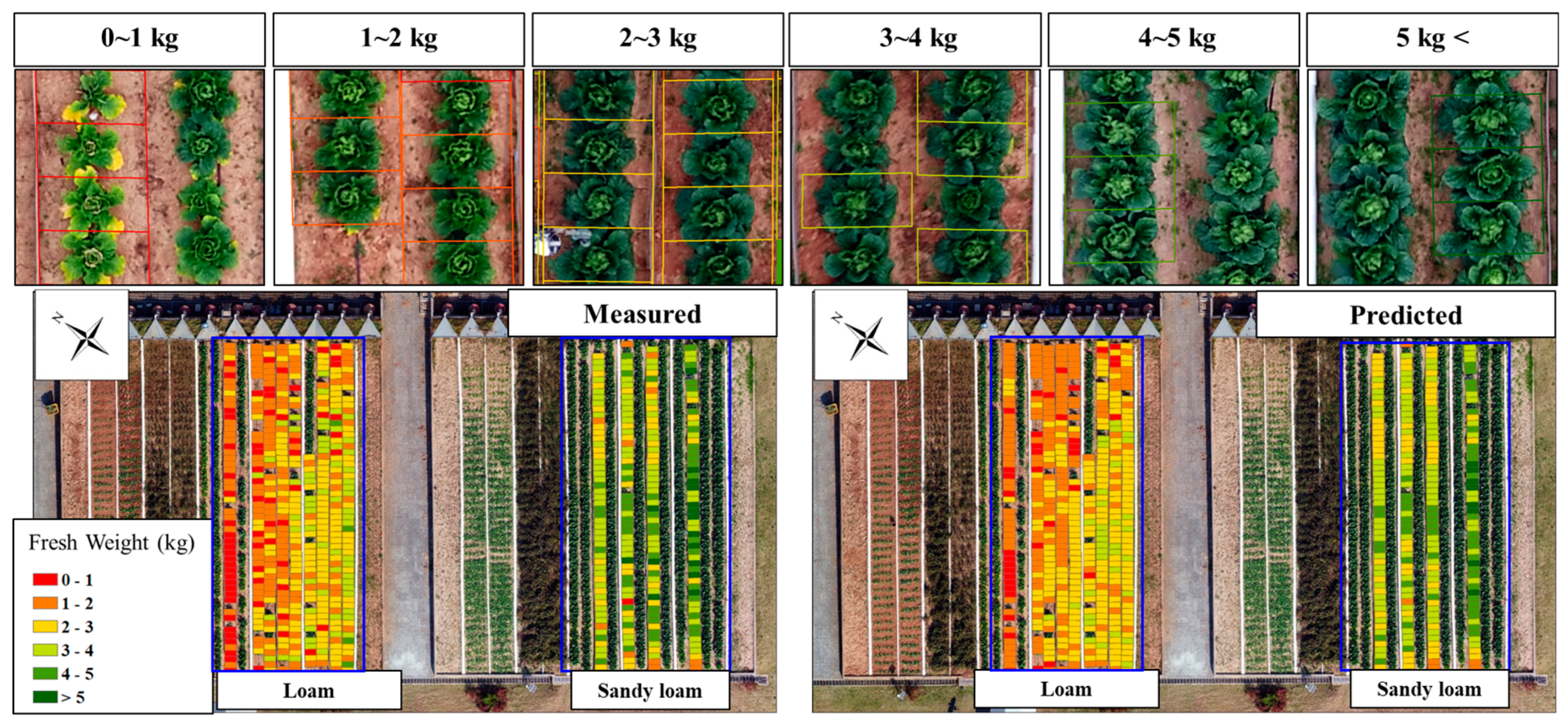
The spatial distribution of measured and DNN model-predicted Napa cabbage fresh weights, as depicted in
Figure 16, reveals the model's ability to capture the variability in fresh weight across different soil types and irrigation conditions. The study area comprises two distinct plots: a loam plot (left) and a sandy loam plot (right). Both measured and predicted weights predominantly fall within the 0-3 kg range in the non-irrigated loam plot, while the irrigated sandy loam plot demonstrates a wider distribution with a greater proportion of Napa cabbages in the 3-5 kg range. This highlights the significant influence of soil type and irrigation on Napa cabbage growth and fresh weight.
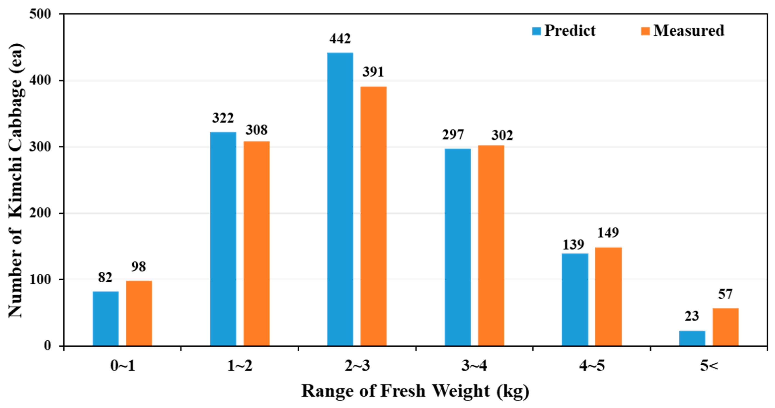
Figure 17 further elucidates this relationship by comparing the distribution of predicted and measured fresh weights across six weight categories for 680 Napa cabbages surveyed in the field and 625 randomly sampled individual fresh weights. While the DNN model demonstrates good agreement with measured data in the 1-2 kg and 3-4 kg ranges, discrepancies are observed in the 2-3 kg and >5 kg ranges, indicating potential areas for model refinement. Specifically, the model tends to overestimate the number of Napa cabbages in the 2-3 kg range and underestimate those in the >5 kg range.
Table 5 offers a comprehensive overview of the predicted fresh weight distribution across the entire test field, highlighting the influence of soil type and irrigation on Napa cabbage growth and fresh weight. The observed lower predicted fresh weights in the non-irrigated loam plot, compared to the more uniform distribution in the irrigated sandy loam plot, underscore the significant impact of these factors on cabbage development.
In conclusion, the DNN model demonstrates significant potential as a tool for predicting Napa cabbage fresh weight, effectively capturing the spatial variability influenced by soil type and irrigation conditions. The model's ability to accurately predict fresh weight for the majority of Napa cabbages, while identifying areas for improvement in specific weight ranges, highlights its potential for enhancing precision agriculture practices in Napa cabbage cultivation. Further research is warranted to refine the model's accuracy under varying environmental conditions and across different Napa cabbage varieties, thereby solidifying its role as a valuable tool for optimizing harvest timing and resource allocation in Napa cabbage production.
5. Discussion
This study investigated the application of three AI algorithms—DNN, SVM, and RF—to predict Napa cabbage fresh weight using UAV-based multi-sensor data. The DNN model, trained on data collected during the heading stage (DAP 42), demonstrated the highest accuracy and stability, suggesting that the Napa cabbage canopy's state at this stage is a robust predictor of final fresh weight.
While the model trained on October 6 (DAP 35, also in the heading stage) showed good performance, it was slightly less accurate than the DAP 42 model. This discrepancy may be attributed to individual variations in growth rate, as some plants continue to increase leaf number and area during this period.
The prediction accuracy decreased slightly for the model trained on October 27 (DAP 56), approaching harvest. This could be due to senescence of outer leaves and reduced photosynthetic capacity, affecting the vegetation index and subsequent fresh weight prediction.
The lowest accuracy was observed for the model trained during the seedling stage (DAP 9). This early stage is characterized by numerous variables influencing growth, making fresh weight prediction more challenging.
Overall, the study revealed that the most accurate predictions were achieved using data collected 3-4 weeks before harvest. The DNN model generally performed well in predicting fresh weight distribution, but tended to underestimate weights exceeding 5 kg. This underestimation might be due to the limited number of large Napa cabbages in the dataset and the saturation of vegetation indices at high chlorophyll concentrations, hindering the model's ability to differentiate these individuals.
Despite this limitation, the model accurately predicted fresh weight for smaller Napa cabbages, offering valuable insights for yield prediction and identifying underperforming plants. This information can aid in predicting potential yield approximately four weeks before harvest and guide interventions for targeted crop management.
Future research should explore more advanced algorithms, expand the range of studied crops, and incorporate larger and more diverse training datasets to further enhance the model's accuracy and generalizability. This includes investigating techniques to mitigate the underestimation of larger Napa cabbages and adapting the model to various environmental conditions, ultimately contributing to more robust and reliable fresh weight prediction for a wider range of agricultural applications.
6. Conclusion
This study successfully developed a novel approach for predicting Napa cabbage fresh weight by integrating UAV-based multi-sensor data and AI algorithms. High-resolution RGB, multispectral, and TIR imagery, collected throughout the 2020 growing season, were used to extract diverse features including vegetation indices, crop height models, and water stress indicators. Among the three AI models tested (DNN, SVM, and RF), the DNN consistently outperformed the others, achieving high accuracy (R² values of 0.86 and 0.82 for training and testing, respectively) and low error (RMSE of 0.432 kg and 0.465 kg, respectively) for fresh weight prediction. This demonstrates the DNN model's superior ability to capture the complex relationships between Napa cabbage fresh weight and multi-sensor features.
The highest prediction accuracy was achieved during the mid-to-late rosette growth stage (DAP 35-42), highlighting the importance of this period for fresh weight estimation due to stable leaf area and well-developed canopy structure. However, the DNN model tended to underestimate the weight of Napa cabbages exceeding 5 kg, potentially due to limited samples and the saturation effect of vegetation indices at high chlorophyll concentrations. Nevertheless, the overall error rate was less than 5%, confirming the feasibility and effectiveness of the proposed approach for fresh weight prediction.
Spatial analysis of the predicted fresh weights revealed patterns consistent with field observations, demonstrating the model's ability to capture the variability in Napa cabbage growth across different soil types and irrigation conditions. The model accurately reflected the impact of drip irrigation in the sandy loam plot, resulting in a higher proportion of larger Napa cabbages compared to the non-irrigated loam plot.
This study significantly contributes to the field of precision agriculture by showcasing the potential of UAV-based multi-sensor data and AI algorithms for accurate and non-invasive prediction of Napa cabbage fresh weight. The developed DNN model offers a valuable tool for optimizing harvest timing, improving crop management practices, and enhancing supply chain efficiency, ultimately leading to increased profitability and reduced food waste. By enabling early and precise yield estimation, this technology empowers farmers to make informed decisions regarding crop management, contributing to sustainable agricultural practices and food security.
Future research should focus on addressing the limitations identified in this study. Expanding the dataset to include more diverse samples and exploring advanced AI techniques could further improve the model's accuracy and generalizability. Additionally, investigating the model's applicability to other crops and varying environmental conditions would broaden its impact and contribute to the wider adoption of precision agriculture technologies.
7. Patents
This paper has nothing to do with applications for intellectual property rights such as patents.
Author Contributions
Conceptualization, Lee, D.H.; methodology, Lee, D.H. and Park, J.H.; software, Lee, D.H.; validation, Park, J.H.; formal analysis, Lee, D.H.; investigation, Lee, D.H. and Park, J.H.; resources, Lee, D.H. and Park, J.H.; data curation, Lee, D.H.; writing—original draft preparation, Lee, D.H.; writing—review and editing, Park, J.H.; visualization, Lee, D.H.; supervision, Park, J.H.
Funding
This study received no funding.
Data Availability Statement
Not applicable.
Acknowledgments
Not applicable.
Conflicts of Interest
The authors declare no conflicts of interest.
References
- Lobell, D.B.; Schlenker, W.; Costa-Roberts, J. Climate Trends and Global Crop Production since 1980. Science 2011, 333, 616–620. [Google Scholar] [CrossRef]
- Walsh, K.J.; McBride, J.L.; Klotzbach, P.J.; Balachandran, S.; Camargo, S.J.; Holland, G.; Knutson, T.R.; Kossin, J.P.; Lee, T.; Sobel, A. Tropical Cyclones and Climate Change. Wiley Interdiscip. Rev. Clim. Change 2016, 7, 65–89. [Google Scholar] [CrossRef]
- Ummenhofer, C.C.; Meehl, G.A. Extreme Weather and Climate Events with Ecological Relevance: A Review. Philos. Trans. R. Soc. B. 2017, 372, 20160135. [Google Scholar] [CrossRef]
- Sishodia, R.P.; Ray, R.L.; Singh, S.K. Applications of Remote Sensing in Precision Agriculture: A Review. Remote Sens. 2020, 12, 3136. [Google Scholar] [CrossRef]
- Kwaghtyo, D.K.; Eke, C.I. Smart Farming Prediction Models for Precision Agriculture: A Comprehensive Survey. Artif.Intell.Rev. 2023, 56, 5729–5772. [Google Scholar] [CrossRef]
- Kim, I.; Jeong, S.; Jeong, G. An Analysis of the Impact of Changes in Kimchi Imports on the Korean Kimchi Industry. Korean J. Org. Agric. 2022, 30, 151–170. [Google Scholar] [CrossRef]
- Eum, H.L.; Kim, B.; Yang, Y.J.; Hong, S.J. Quality Evaluation and Optimization of Storage Temperature with Eight Cultivars of Kimchi Cabbage Produced in Summer at Highland Areas. Hortic. Sci. Technol. 2013, 31, 211–218. [Google Scholar] [CrossRef]
- Choi, E.J.; Jeong, M.C.; Ku, K.H. Effect of Seasonal Cabbage Cultivar (Brassica Rapa L. Ssp. Pekinesis) on the Quality Characteristics of Salted-Kimchi Cabbages during Storage Period. Korean J. Food Preserv. 2015, 22, 303–313. [Google Scholar] [CrossRef]
- Radoglou-Grammatikis, P.; Sarigiannidis, P.; Lagkas, T.; Moscholios, I. A Compilation of UAV Applications for Precision Agriculture. Comput. Netw. 2020, 172, 107148. [Google Scholar] [CrossRef]
- Tripathi, M.K.; Maktedar, D.D. A Role of Computer Vision in Fruits and Vegetables among various Horticulture Products of Agriculture Fields: A Survey. Inf. Process. Agric. 2020, 7, 183–203. [Google Scholar] [CrossRef]
- De Ocampo, A.L.P.; Montalbo, F.J.P. A Multi-Vision Monitoring Framework for Simultaneous Real-Time Unmanned Aerial Monitoring of Farmer Activity and Crop Health. Smart Agric. Technol. 2024, 8, 100466. [Google Scholar] [CrossRef]
- Mezera, J.; Lukas, V.; Horniaček, I.; Smutný, V.; Elbl, J. Comparison of Proximal and Remote Sensing for the Diagnosis of Crop Status in Site-Specific Crop Management. Sensors 2021, 22, 19. [Google Scholar] [CrossRef] [PubMed]
- Kumar, H.; Srivastava, P.; Lamba, J.; Ortiz, B.V.; Way, T.R.; Sangha, L.; Takhellambam, B.S.; Morata, G.; Molinari, R. Within-Field Variability in Nutrients for Site-Specific Agricultural Management in Irrigated Cornfield. J. ASABE 2022, 65, 865–880. [Google Scholar] [CrossRef]
- Flores, R.; Lázaro, E.; Ramos, E.; Provost, K.; Habib, M. Demand Management in the Supply Chain: A Focus on Agribusiness. In Advances in Manufacturing, Production Management and Process Control: Proceedings of the AHFE 2020 Virtual Conferences on Human Aspects of Advanced Manufacturing, Advanced Production Management and Process Control, and Additive Manufacturing, Modeling Systems and 3D Prototyping, San Diego, CA, USA USA, 16–20 July 2020; pp. 333–340.
- Karthikeyan, L.; Chawla, I.; Mishra, A.K. A Review of Remote Sensing Applications in Agriculture for Food Security: Crop Growth and Yield, Irrigation, and Crop Losses. J. Hydrol. 2020, 586, 124905. [Google Scholar] [CrossRef]
- Shi, Y.; Ji, S.; Shao, X.; Tang, H.; Wu, W.; Yang, P.; Zhang, Y.; Ryosuke, S. Framework of SAGI Agriculture Remote Sensing and its Perspectives in Supporting National Food Security. J. Integr. Agric. 2014, 13, 1443–1450. [Google Scholar] [CrossRef]
- Saranya, T.; Deisy, C.; Sridevi, S.; Anbananthen, K.S.M. A Comparative Study of Deep Learning and Internet of Things for Precision Agriculture. Eng. Appl. Artif. Intell. 2023, 122, 106034. [Google Scholar] [CrossRef]
- Benos, L.; Tagarakis, A.C.; Dolias, G.; Berruto, R.; Kateris, D.; Bochtis, D. Machine Learning in Agriculture: A Comprehensive Updated Review. Sensors 2021, 21, 3758. [Google Scholar] [CrossRef] [PubMed]
- Lee, D.; Shin, H.; Park, J. Developing a P-NDVI Map for Highland Kimchi Cabbage using Spectral Information from UAVs and a Field Spectral Radiometer. Agronomy 2020, 10, 1798. [Google Scholar] [CrossRef]
- Nevavuori, P.; Narra, N.; Linna, P.; Lipping, T. Crop Yield Prediction using Multitemporal UAV Data and Spatio-Temporal Deep Learning Models. Remote Sens. 2020, 12, 4000. [Google Scholar] [CrossRef]
- Hassan, M.A.; Yang, M.; Rasheed, A.; Yang, G.; Reynolds, M.; Xia, X.; Xiao, Y.; He, Z. A Rapid Monitoring of NDVI Across the Wheat Growth Cycle for Grain Yield Prediction using a Multi-Spectral UAV Platform. Plant Sci. 2019, 282, 95–103. [Google Scholar] [CrossRef]
- Messina, G.; Modica, G. Applications of UAV Thermal Imagery in Precision Agriculture: State of the Art and Future Research Outlook. Remote Sens. 2020, 12, 1491. [Google Scholar] [CrossRef]
- Zhang, C.; Kovacs, J.M. The Application of Small Unmanned Aerial Systems for Precision Agriculture: A Review. Precis. Agric. 2012, 13, 693–712. [Google Scholar] [CrossRef]
- Lee, D.; Kim, H.; Park, J. UAV, a Farm Map, and Machine Learning Technology Convergence Classification Method of a Corn Cultivation Area. Agronomy 2021, 11, 1554. [Google Scholar] [CrossRef]
- Kwak, G.; Park, N. Unsupervised Domain Adaptation with Adversarial Self-Training for Crop Classification using Remote Sensing Images. Remote Sens. 2022, 14, 4639. [Google Scholar] [CrossRef]
- Go, S.; Lee, D.; Na, S.; Park, J. Analysis of Growth Characteristics of Kimchi Cabbage using Drone-Based Cabbage Surface Model Image. Agriculture 2022, 12, 216. [Google Scholar] [CrossRef]
- Zhu, W.; Sun, Z.; Yang, T.; Li, J.; Peng, J.; Zhu, K.; Li, S.; Gong, H.; Lyu, Y.; Li, B.; et al. Estimating Leaf Chlorophyll Content of Crops Via Optimal Unmanned Aerial Vehicle Hyperspectral Data at Multi-Scales. Comput.Electron.Agric. 2020, 178, 105786. [Google Scholar] [CrossRef]
- Lee, D.; Jeong, C.; Go, S.; Park, J. Evaluation of Applicability of RGB Image using Support Vector Machine Regression for Estimation of Leaf Chlorophyll Content of Onion and Garlic. Korean J. Remote Sens. 2021, 37, 1669–1683. [Google Scholar] [CrossRef]
- Maimaitijiang, M.; Sagan, V.; Sidike, P.; Hartling, S.; Esposito, F.; Fritschi, F.B. Soybean Yield Prediction from UAV using Multimodal Data Fusion and Deep Learning. Remote Sens.Environ. 2020, 237, 111599. [Google Scholar] [CrossRef]
- Kim, D.; Yun, H.S.; Jeong, S.; Kwon, Y.; Kim, S.; Lee, W.S.; Kim, H. Modeling and Testing of Growth Status for Chinese Cabbage and White Radish with UAV-Based RGB Imagery. Remote Sens. 2018, 10, 563. [Google Scholar] [CrossRef]
- Killeen, P.; Kiringa, I.; Yeap, T.; Branco, P. Corn Grain Yield Prediction using UAV-Based High Spatiotemporal Resolution Imagery, Machine Learning, and Spatial Cross-Validation. Remote Sens. 2024, 16, 683. [Google Scholar] [CrossRef]
- Shahi, T.B.; Xu, C.; Neupane, A.; Guo, W. Recent Advances in Crop Disease Detection using UAV and Deep Learning Techniques. Remote Sens. 2023, 15, 2450. [Google Scholar] [CrossRef]
- Kamilaris, A.; Prenafeta-Boldú, F.X. Deep Learning in Agriculture: A Survey. Comput.Electron.Agric. 2018, 147, 70–90. [Google Scholar] [CrossRef]
- Woebbecke, D.M.; Meyer, G.E.; Von Bargen, K.; Mortensen, D.A. Color Indices for Weed Identification Under various Soil, Residue, and Lighting Conditions. Trans.ASAE 1995, 38, 259–269. [Google Scholar] [CrossRef]
- Ostu, N. A Threshold Selection Method from Gray-Level Histograms. IEEE Trans. Syst. Man Cybern. 1979, 9, 62–66. [Google Scholar] [CrossRef]
- Bendig, J.; Bolten, A.; Bennertz, S.; Broscheit, J.; Eichfuss, S.; Bareth, G. Estimating Biomass of Barley using Crop Surface Models (CSMs) Derived from UAV-Based RGB Imaging. Remote Sens. 2014, 6, 10395–10412. [Google Scholar] [CrossRef]
- Jones, H.G. Use of Infrared Thermometry for Estimation of Stomatal Conductance as a Possible Aid to Irrigation Scheduling. Agric. For. Meteorol. 1999, 95, 139–149. [Google Scholar] [CrossRef]
- Gitelson, A.A.; Viña, A.; Ciganda, V.; Rundquist, D.C.; Arkebauer, T.J. Remote Estimation of Canopy Chlorophyll Content in Crops. Geophys.Res.Lett. 2005, 32. [Google Scholar] [CrossRef]
- Gitelson, A.A.; Kaufman, Y.J.; Stark, R.; Rundquist, D. Novel Algorithms for Remote Estimation of Vegetation Fraction. Remote Sens.Environ. 2002, 80, 76–87. [Google Scholar] [CrossRef]
- Vincini, M.; Frazzi, E.; D’Alessio, P. A Broad-Band Leaf Chlorophyll Vegetation Index at the Canopy Scale. Precis. Agric. 2008, 9, 303–319. [Google Scholar] [CrossRef]
- Jordan, C.F. Derivation of Leaf-area Index from Quality of Light on the Forest Floor. Ecology 1969, 50, 663–666. [Google Scholar] [CrossRef]
- Gitelson, A.A.; Kaufman, Y.J.; Merzlyak, M.N. Use of a Green Channel in Remote Sensing of Global Vegetation from EOS-MODIS. Remote Sens.Environ. 1996, 58, 289–298. [Google Scholar] [CrossRef]
- Pinty, B.; Verstraete, M.M. GEMI: A Non-Linear Index to Monitor Global Vegetation from Satellites. Vegetatio 1992, 101, 15–20. [Google Scholar] [CrossRef]
- Rouse, J.; Haas, R.; Schell, J.; Deering, D. Monitoring Vegetation Systems in the Great Plains with ERTS; NASA. Goddard Space Flight Center 3d ERTS-1 Symp.; 1973; Volume 1, pp. 309–317. Available online: http://hdl.handle.net/2060/19740022614 (accessed on 2 July 2024).
- Camps-Valls, G.; Bruzzone, L.; Rojo-Álvarez, J.L.; Melgani, F. Robust Support Vector Regression for Biophysical Variable Estimation from Remotely Sensed Images. IEEE Geosci. Remote Sens. Lett. 2006, 3, 339–343. [Google Scholar] [CrossRef]
- Breiman, L. Random Forests. Machine Learning 2001, 45, 5–32. [Google Scholar] [CrossRef]
Figure 1.
Layout of the Napa cabbage Cultivation Test Field at the National Institute of Agricultural Sciences. Rep. of Korea.
Figure 1.
Layout of the Napa cabbage Cultivation Test Field at the National Institute of Agricultural Sciences. Rep. of Korea.
Figure 2.
Fall Napa cabbage Growth Stages and UAV Image Acquisition Timeline (2020).
Figure 2.
Fall Napa cabbage Growth Stages and UAV Image Acquisition Timeline (2020).
Figure 3.
Workflow for UAV-Based RGB, Multispectral (MSP) and Thermal Infrared (TIR) Imaging, AI Modeling, and Analysis for Napa cabbage Monitoring and Fresh Weight Prediction in Precision Agriculture.
Figure 3.
Workflow for UAV-Based RGB, Multispectral (MSP) and Thermal Infrared (TIR) Imaging, AI Modeling, and Analysis for Napa cabbage Monitoring and Fresh Weight Prediction in Precision Agriculture.
Figure 4.
Geometric Correction of UAV Imagery Using Ground Control Points (GCPs) and GPS-RTK.
Figure 4.
Geometric Correction of UAV Imagery Using Ground Control Points (GCPs) and GPS-RTK.
Figure 5.
Radiometric Calibration of Multispectral Sensor Data Using Reflectance Panels and Downwelling Light Sensor (DLS).
Figure 5.
Radiometric Calibration of Multispectral Sensor Data Using Reflectance Panels and Downwelling Light Sensor (DLS).
Figure 6.
Spatial Distribution of Napa cabbage Sampling Points for Fresh Weight and Crop Height Measurements within the Test Field.
Figure 6.
Spatial Distribution of Napa cabbage Sampling Points for Fresh Weight and Crop Height Measurements within the Test Field.
Figure 7.
Sequential Extraction of Vegetation Area from UAV RGB Imagery: (a) Original RGB image, (b) Excess Green (ExG) index image, (c) Binary mask generated by Otsu's thresholding on the ExG image, and (d) Final delineation of vegetation area.
Figure 7.
Sequential Extraction of Vegetation Area from UAV RGB Imagery: (a) Original RGB image, (b) Excess Green (ExG) index image, (c) Binary mask generated by Otsu's thresholding on the ExG image, and (d) Final delineation of vegetation area.
Figure 8.
Grid-Based Segmentation of Individual Napa cabbage Objects in UAV Imagery: (a) Identification of center points for each cabbage object, (b) Generation of initial ellipses based on planting distance (Minor), row spacing (Major), and orientation (θ), (c) Adjustment of ellipses to conform to individual cabbage locations, (d) Conversion of adjusted ellipses into rectangular grids, and (e) Final segmentation of individual cabbage objects.
Figure 9.
Architecture of the Deep Neural Network (DNN) Model for Predicting Napa cabbage Fresh Weight.
Figure 9.
Architecture of the Deep Neural Network (DNN) Model for Predicting Napa cabbage Fresh Weight.
Figure 10.
Comparison of R² values for DNN, SVM, and RF models for Napa cabbage fresh weight prediction using training and test datasets across different survey dates (DAP).
Figure 10.
Comparison of R² values for DNN, SVM, and RF models for Napa cabbage fresh weight prediction using training and test datasets across different survey dates (DAP).
Figure 11.
Comparison of RMSE for DNN, SVM, and RF models in Predicting Napa cabbage Fresh Weight using Training and Test Datasets Across Different Survey Dates (DAP).
Figure 11.
Comparison of RMSE for DNN, SVM, and RF models in Predicting Napa cabbage Fresh Weight using Training and Test Datasets Across Different Survey Dates (DAP).
Figure 12.
Comparison of Overfitting in DNN, SVM, and RF Models for Napa cabbage Fresh Weight Prediction: Differences in R² and RMSE between Training and Test Datasets Across Survey Dates (DAP).
Figure 12.
Comparison of Overfitting in DNN, SVM, and RF Models for Napa cabbage Fresh Weight Prediction: Differences in R² and RMSE between Training and Test Datasets Across Survey Dates (DAP).
Figure 13.
Scatterplot of Predicted vs. Measured Napa cabbage Fresh Weight Using DNN Model for Training and Test Datasets
Figure 13.
Scatterplot of Predicted vs. Measured Napa cabbage Fresh Weight Using DNN Model for Training and Test Datasets
Figure 14.
Scatterplot of Predicted vs. Measured Napa cabbage Fresh Weight Using SVM Model for Training and Test Datasets
Figure 14.
Scatterplot of Predicted vs. Measured Napa cabbage Fresh Weight Using SVM Model for Training and Test Datasets
Figure 15.
Scatterplot of Predicted vs. Measured Napa cabbage Fresh Weight Using RF Model for Training and Test Datasets
Figure 15.
Scatterplot of Predicted vs. Measured Napa cabbage Fresh Weight Using RF Model for Training and Test Datasets
Figure 16.
Spatial Distribution of Measured and Predicted Napa cabbage Fresh Weight (kg) in Loam and Sandy Loam Soil Plots using the DNN model as of October 13, 2020 (DAP 42).
Figure 16.
Spatial Distribution of Measured and Predicted Napa cabbage Fresh Weight (kg) in Loam and Sandy Loam Soil Plots using the DNN model as of October 13, 2020 (DAP 42).
Figure 17.
Comparison of Predicted and Measured Fresh Weight Distribution of Napa cabbage Across Different Weight Ranges
Figure 17.
Comparison of Predicted and Measured Fresh Weight Distribution of Napa cabbage Across Different Weight Ranges
Table 1.
UAV Imagery Acquisition Dates for Fall Napa cabbage Growth Monitoring (2020).
Table 1.
UAV Imagery Acquisition Dates for Fall Napa cabbage Growth Monitoring (2020).
| Year |
Date (mm/dd) |
| 2020 |
9/1, 9/10, 9/15, 9/24, 10/6, 10/13, 10/20, 10/27, 11/9 |
Table 2.
Independent Variables Derived from RGB, Multispectral, and Thermal Infrared Imagery for Cabbage Fresh Weight Prediction Models.
Table 2.
Independent Variables Derived from RGB, Multispectral, and Thermal Infrared Imagery for Cabbage Fresh Weight Prediction Models.
| Sensor type |
Vegetation Index |
Equation |
Reference |
| RGB |
VF (Vegetation Fraction) |
VF = (Area of each Napa cabbage object) / (Grid area) |
- |
| CHM (Crop Height Model) |
CHM = DSM_(growth stage) - DSM_(pre-planting) |
[36] |
| Multi Spectral |
CIRE
(Red Edge Chlorophyll Index) |
CIRE = (RN / RRE) - 1
|
[38] |
VARI
(Visible Atmospherically
Resistant Index) |
VARI = (RG- RR) / (RG+ RR)
|
[39] |
| CVI (Chlorophyll Vegetation Index) |
CVI = (RN / RG) x (RR / RG)
|
[40] |
| SR (Simple Ratio) |
SR = (RN / RG) |
[41] |
GNDVI
(Green Normalized Difference
Vegetation Index) |
GNDVI = (RN- RG) / (RN+ RG)
|
[42] |
CIGreen
(Green Chlorophyll Index) |
CIGreen = (RN / RG) - 1
|
[38] |
GEMI
(Global Environmental
Monitoring Index) |
GEMI = n x [(1-0.25n) x ( RR – 0.125)]/(1 - RR)
*n = [( RN2 - RR2) + 1.5 x RN + 0.5 x RR]/ (RN + RR +0.5)
|
[43] |
NDVI
(Normalized Difference
Vegetation Index) |
NDVI = (RN- RR) / (RN+ RR)
|
[44] |
| Thermal Infrared |
CWSI
(Crop Water Stress Index) |
CWSI = (T - Tc) / (Th - Tc) |
[37] |
Table 3.
Performance of AI Models for Predicting Napa cabbage Fresh Weight across Different Survey Dates (September 10 - October 27, 2020).
Table 3.
Performance of AI Models for Predicting Napa cabbage Fresh Weight across Different Survey Dates (September 10 - October 27, 2020).
| Model |
Data Set |
Metrics |
Date |
10
Sep |
15
Sep |
24
Sep |
6
Oct |
13
Oct |
20
Oct |
27
Oct |
| DNN |
Train |
R2
|
0.52 |
0.53 |
0.70 |
0.81 |
0.84* |
0.83 |
0.80 |
| Test |
0.50 |
0.52 |
0.67 |
0.79 |
0.82 |
0.81 |
0.79 |
| RF |
Train |
0.44 |
0.46 |
0.66 |
0.73 |
0.75 |
0.75 |
0.74 |
| Test |
0.43 |
0.43 |
0.59 |
0.65 |
0.69 |
0.65 |
0.64 |
| SVM |
Train |
0.45 |
0.45 |
0.65 |
0.76 |
0.78 |
0.77 |
0.73 |
| Test |
0.40 |
0.43 |
0.63 |
0.70 |
0.73 |
0.72 |
0.71 |
| DNN |
Train |
RMSE
(kg) |
1.04 |
1.01 |
0.69 |
0.47 |
0.43 |
0.44 |
0.49 |
| Test |
1.07 |
1.04 |
0.74 |
0.52 |
0.47 |
0.48 |
0.53 |
| RF |
Train |
1.09 |
1.05 |
0.66 |
0.52 |
0.49 |
0.50 |
0.52 |
| Test |
1.22 |
1.21 |
0.90 |
0.79 |
0.71 |
0.79 |
0.80 |
| SVM |
Train |
1.18 |
1.17 |
0.79 |
0.58 |
0.55 |
0.57 |
0.64 |
| Test |
1.27 |
1.22 |
0.83 |
0.70 |
0.63 |
0.66 |
0.68 |
Table 4.
Fresh Weight Bias Analysis of DNN, SVM, and RF Models for Overall Napa cabbage and by Weight Section
Table 4.
Fresh Weight Bias Analysis of DNN, SVM, and RF Models for Overall Napa cabbage and by Weight Section
Range of
Fresh Wight |
Models |
| DNN |
RF |
SVM |
| < 1 |
-0.021 |
-0.002 |
-0.015 |
| 1∼2 |
-0.212 |
-0.229 |
-0.335 |
| 2∼3 |
0.086 |
-0.007 |
-0.026 |
| 3∼4 |
0.354 |
0.200 |
0.219 |
| 4∼5 |
0.365 |
0.227 |
0.464 |
| > 5 |
0.109 |
0.541 |
0.88 |
| All Range |
0.008 |
0.031 |
0.041 |
Table 5.
Comparison of Measured and Predicted Fresh Weight of Kimchi Cabbage Harvested from Loam and Sandy Loam Plots in 2020
Table 5.
Comparison of Measured and Predicted Fresh Weight of Kimchi Cabbage Harvested from Loam and Sandy Loam Plots in 2020
| Year |
Number of Kimchi cabbage |
Measured Fresh Weight (kg) [A] |
Predicted Fresh Weight (kg) [B] |
Error rate (%)
[1-B/A×100] |
| 2020 |
1,305 |
3,507 |
3,413 |
2.69 |
|
Disclaimer/Publisher’s Note: The statements, opinions and data contained in all publications are solely those of the individual author(s) and contributor(s) and not of MDPI and/or the editor(s). MDPI and/or the editor(s) disclaim responsibility for any injury to people or property resulting from any ideas, methods, instructions or products referred to in the content. |
© 2024 by the authors. Licensee MDPI, Basel, Switzerland. This article is an open access article distributed under the terms and conditions of the Creative Commons Attribution (CC BY) license (http://creativecommons.org/licenses/by/4.0/).
