1. Introduction
Entropy is defined as the loss of information in a time series or signal, which quantifies the amount of uncertainty regarding the order of an output signal [
1]. Within the past twenty years, the use of entropy methods to define periodicity or regularity in human physiological and biomechanical data has become prevalent [
2]. Two commonly used methods for evaluating biological time-series data are approximate entropy (ApEn) and sample entropy (SampEn). Because entropy quantifies the likelihood of the next state of a system, based on what is known about the present state of a time series, it has been used to identify physiological changes with aging [
3,
4], cardiovascular status [
5,
6,
7], and respiratory pathology [
1,
8,
9]. Entropy calculations can take more forms, but ApEn and SampEn have been particularly useful for understanding more about the changes in postural control systems [
10,
11,
12,
13,
14,
15], human gait mechanics [
16,
17], and standing balance [
2,
10,
13,
18,
19,
20,
21].
In 1991, Pincus used ApEn to measure signal regularity and quantify levels of complexity within a time series; low values of ApEn tended to indicate a more regular and predictable signal and larger values suggested greater unpredictability [
22]. With biological data sets, in general, but human movement in particular, quantifying levels of complexity has become important. For example, newer motor control theories, e.g., dynamical systems theory, do not consider variability in movement as an error [
17]. Dynamical systems theory considers the complexity of movement patterns, i.e., variability, to be associated with system stability.
ApEn and SampEn have been shown to demonstrate the state and changes in the complexity of various physiological signals related to seated postural control in individuals with chronic stroke [
23], electrocardiograms [
24], electroencephalograms (EEG) [
25], heart rate variability [
26,
27], and neural respiratory time series [
8]. In complex systems, e.g., cardiac, respiratory, somatosensory, etc., lower ApEn values reflect systems that are persistent, repetitive, and predictive, with apparent patterns that repeat themselves throughout the series [
6,
28]. So, it is more appropriate to use terms like probability, predictability, and regularity, when describing the nature of a measurable complex system. In summary, the use of ApEn and SampEn was not meant to comprehensively analyze complex systems but to statistically quantify the dynamics of time series related to complex systems [
29].
Based on the work by Pincus [
26,
28] and Cavanaugh et al. [
18,
19], we can assume that the diverse and interconnected components, i.e., visual, vestibular, and somatosensory, of the complex healthy human postural control system are capable of adapting to a wide variety of task demands, i.e., internal and external perturbations. Thus, this postural control system, when allowed to operate with minimal constraints, i.e., at rest during quiet standing, demonstrates an output, e.g., the center of pressure excursion, that appears to fluctuate in a relatively random (nonlinear) fashion that reflects its readiness to respond to internal and external perturbations. However, it has been shown that the anterior-posterior (AP) and medial-lateral (ML) oscillations are relatively small and random and are not sensitive enough to detect subtle alterations in postural control related to cerebral concussion [
10]. Based on Pincus’ groundbreaking work, the use of ApEn in the assessment of postural sway in healthy [
10] and concussed young adults has provided insight into the control of static and dynamic balance [
18,
19]. Cavanaugh et al. [
18] reported that ApEn values for the AP and ML COP time series generally declined immediately after injury (i.e., concussion) in both steady and unsteady injured athletes suggesting a postural control system that was more constrained after injury. Interestingly, depressed ApEn values were still evident 48 to 96 hours after injury although postural instability had resolved.
Both ApEn and SampEn methods utilize three input parameters: N is the data length, m is the length of the window of the different vector comparisons (often referred to as the embedding dimension, vector length, pattern length, segment length, or pattern window), and r is the tolerance (sometimes referred to as radius or tolerance window), i.e., function criterion of similarity or type of signal filter. Both indices quantify complexity in the data by looking at the difference in m point vs. m+1 point patterns, over the N point data length.
ApEn measures the logarithmic probability that nearby pattern runs remain close in the next incremental comparison [
19]. Given the input parameters, ApEn (
m, r, and
N) [
26] is denoted by the expression:
(
r) is the probability that two sequences are similar for
m points with self-counting and
(
r) is the probability that two sequences are similar for
m + 1 matches with self-counting. Self-counting suggests that given one template the segment in the sequence is compared to all the blocks in the sequence, including itself. For ApEn, self-counting is needed in the calculation of conditional probabilities to ensure the logarithms remain finite. Statistically, selecting
m and
r as input parameters would be the equivalent of dividing the space of states into cells of width
r, to estimate the conditional probabilities of the
m-th order [
19]. Greater values of
m and smaller values of
r describe details of sharper, more probabilistic parameters [
19]. However, when dealing with stochastic processes, the analysis of conditional probabilities causes large values of
m or minimal values of
r to produce statistically low estimates. Ultimately, the value of the estimate depends on
m and
r. Pincus [
28] suggested taking
m as 2 and
r as 0.2 * SD
x, where SD
x is the standard deviation of the original data <
x(n)>, i.e.,
Pincus [
28] has offered that one of the advantages of ApEn is that the algorithm was finite for stochastic, noisy deterministic, and composite processes, i.e., models for complex biological systems. ApEn can differentiate between different mixed methods of deterministic and random components occurring with a different probability and is robust to outliers because the pattern formed by wild points will rarely be repeated in the waveform [
7]. It has been demonstrated that an increasing ApEn corresponds to intuitively increasing process complexity in a biological modeling platform. However, the limitations of ApEn include that relative consistency is not guaranteed, and depending on the value of
r, the ApEn values will change [
1]. Additionally, the value of ApEn depends on the length of the data series. Lastly, the self-counting aspect of the algorithm creates a statistical bias that particularly impacts situations with small data sets, that is when only a few or even no matches are present, the entropic result is biased toward zero [
1].
Richman and Moorman [
6] introduced SampEn as an alternative to counteract the limitations of ApEn, claiming that SampEn, as a statistical alternative, solved the self-counting problem eliminating the bias associated with ApEn. Eliminating self-counting is justified given that entropy is conceived as a measure of the rate of information production. ApEn uses the whole series to determine its value, needing only a template vector to find a match of length
m + 1 to be defined [
19]. SampEn contrasts with ApEn, where each template vector must find a match to be determined [
2]. SampEn (
m, r, and
N) is defined as the negative value of the logarithm of the conditional probability that two similar sequences of
m points remain identical at the next point
m + 1, counting each vector over all the other vectors except on itself [
19].
is the probability that two sequences are similar for
m points,
is the probability that two sequences are similar for
m + 1 matches, where the ratio is a conditional probability. The use of SampEn appears to quantify regularity more effectively and eliminates many of the problems associated with ApEn [
6].
SampEn maintains the relative consistency and is also mostly independent of the length of the time series [
6]. SampEn was created to address the bias and inconsistencies of ApEn, yet both methods retain similarities [
6]. There is no consensus on which method is preferable, but one’s choice should be dependent on the research question and time series being evaluated.
When using ApEn and SampEn important consideration must be given to parameter selection, as these choices may have the greatest impact on the final entropy value even in the presence of noise [
30]. Given a time series with
N data points, the calculation of entropy requires
a priori determination of two unknown parameters, embedding dimension,
m, and threshold,
r [
31]. Multiple pairings of parameter selections allow one to examine relative consistency where a better discrimination capacity can be accomplished. Incorrect parameter choice, and lack of due diligence in selecting
m, r, and
N can undermine the interpretation and application of entropy results.
According to Yentes et al. [
17] when the sampling rate is too high, i.e., frequency collection rates greater than 1000 Hz, redundancy likely exists within the data, which tends to artificially reduce entropy values [
21]. Redundancy, i.e., repetitiveness of, or repeating, values, results in smaller entropy values and more signal regularity secondary to the counting of repeated matches. The redundant data problem can be solved by downsampling overly redundant time series data sets. Although downsampling removes real data, sensitivity analyses have demonstrated that the loss of data does not impact the subsequent application of the revised data set [
12,
16]. Previous studies have demonstrated the link between entropy and sampling rate. Powell et al [
32] simulated different sampling rates by resampling ankle joint angle time series and found that higher sampling rates significantly reduced ApEn values. Conversely, results from Rhea et al. [
33] suggest that excessive downsampling, e.g., to 25 Hz, artificially altered the standing center of pressure displacement and velocity SampEn values.
Based on the literature, it is clear that the appropriate selections of
N,
m, and
r are critical for computing ApEn and SampEn values that can enhance the interpretation of inherently non-linear biological time series. Further, there is a lack of agreement on best practices. Therefore, the purposes of this research were to: 1) examine and evaluate the effect of altering input tolerance,
r, on ApEn and SampEn values related to the center of pressure time series during quiet standing postures, i.e., feet together and tandem standing, and under eyes-open and eyes-closed conditions, and 2) assess which entropy measure was less biased and most consistent. Specific center of pressure metrics were chosen because they represent a single measurement of the complex postural control mechanism used to maintain balance and incorporate essential somatosensory and neuromotor inputs that influence stability [
21].
4. Discussion
Understanding how individuals respond to different postural, both static and dynamic, conditions and utilizing the best method to measure those conditions is important when comparing how a healthy nervous system responds versus how a brain-injured individual responds to the same conditions. Previous research that has examined children and adults with mild traumatic brain injury, e.g., concussion, has suggested that the use of the center of pressure (COP) data can be useful in delineating a normal from an abnormal response to the perturbations of static and dynamic balance [
10,
13,
14,
18,
40,
41]. Since it has been shown that the COP time series is non-linear, traditional methods of assessing various COP parameters, e.g., statistical use of means and standard deviation, have not been effective [
41]. Previous work using non-linear metrics, such as approximate and sample entropy, to study normal and pathological balance has been useful [
3,
18,
19,
44,
45,
46]. However, a consensus on the optimal input parameter, i.e.,
N,
m, and
r, selection for the calculation of ApEn and SampEn has not yet been established. Previous work by Yentes et al. [
16,
17,
30] has examined this challenge and made recommendations relative to gait data [
16,
30] and short data sets [
17], but there is a paucity of research on this matter in investigations involving standing postural control. In our laboratory, Tipton et al. [
21] measured the center of pressure of healthy college-aged participants under various quiet standing postures and used ApEn to characterize the time series, but their method was limited by an overly redundant data set and included the determination of the tolerance window,
r, that was atypical. Based on the need described in the literature for more work investigating the diverse application of ApEn and SampEn analyses, and the methodological limitations of the previous research in our laboratory, the primary purpose of this study was to compare ApEn and SampEn under various stability conditions and examine the effects of different tolerance window values. The results revealed: 1) that even though SampEn tended to yield lower mean values than ApEn, both indices equally quantified the regularity of a COP time series in both the anterior-posterior and medial-lateral directions; 2) both ApEn and SampEn effectively differentiated a more stable quiet standing posture, i.e., eyes open feet together, from less stable standing postures, i.e., eyes open and eyes closed tandem standing postures; and 3), the selection of
r had a relatively consistent effect with both entropic statistical analyses.
It has been demonstrated that high sampling rates reduce entropy values, likely since higher rates are well above the frequency of the tested behavior creating an artificial increase in the number of matches [
12,
30]. We used Tipton et al.’s [
21] raw COP time series but modified it because their decision not to reduce data redundancy may have resulted in ApEn values that were biased, i.e. greater predictability. Therefore, we chose to downsample the COP time series data which allowed us to use a more accepted method for determining tolerance windows. Others have demonstrated the importance of how data management is handled and interpreted. For example, Rhea et al. [
33] noted that downsampling from 100 Hz to 50 Hz and 25 Hz produced a dataset that appeared to be linearly less regular, i.e., increasing SampEn. They cautioned that researchers must identify how much change is driven by the neuromotor system and how much is a function of the data processing technique. Lubetsky et al. [
12] noted that since postural sway typically lies between 0.15 and 0.4 Hz (and as high as 3 Hz) a sampling rate of 25 Hz should be sufficient to detect time series patterns and better reflect the underlying postural sway pattern. Thus, they were interested in evaluating how sample entropy of COP time series data sampled at 100 Hz (
N = 2000) from prolonged standing tasks on normal and compliant surfaces would be affected by downsampling by 2, 3, and 4. They found that although downsampling increased SampEn values, it had an insignificant effect on the comparisons to the original datasets. However, they concluded that if such procedures are performed by other researchers, they should be well justified. Yentes et al. [
17] recommended, as best practice, that practitioners not exceed sampling data beyond 1000 Hz, but that a prior power spectral density analysis might be considered to assist in selecting an appropriate sampling rate. In the present study, our initial entropy estimates based on a 1200 Hz data collection rate yielded very low entropy values between 0.005 and 0.030. Therefore, we concluded that downsampling was necessary for the processing of our entropy results. We found that, when using 1,800-point arrays, the raw COP waveforms were observationally nearly identical when comparing unfiltered data to the downsampled data and that the entropy values that resulted, i.e., average ApEn and SampEn, ranged from 0.08 to 0.90; values consistent with other published works.
Incorrect parameter selection, i.e., vector length,
m, tolerance or threshold window,
r, and data length,
N), regardless of the biological time series being considered, can undermine the ApEn and SampEn discrimination capacity [
47]. For this study, the embedding dimension,
m = 2, and dataset length,
N, were fixed input parameters. We wanted to focus our attention on assessing entropy outcomes relative to changes in the tolerance window since this parameter may have the greatest influence on the calculation of entropy [
30] and is considered one of the most difficult to select [
16]. Selecting a tolerance window too small limits the number of matches found and selecting too large a window could lead to too many matches found and increase the probability [
30]. Many approaches to calculating
r have been suggested, including utilizing the standard deviation (SD) of the whole time series [
26,
45], the standard error of the entropy values [
48], predefined tolerance levels [
49,
50], and using a heuristic stochastic model [
47]. Typically, the tolerance window is calculated as
r times the standard deviation of the time series [
26]. However, many researchers have reported determining, and using,
r as 0.2 * SD, with the rationale that it was commonly used in previous research. Yentes et al. [
30] recommended that researchers try multiple
r values, and if using the default method, i.e., r * SD, test the relative consistency of
r = 0.15, 0.25, and 0.30 * SD. For this study, we calculated ApEn and SampEn related to the anterior-posterior and medial-lateral COP excursions during a variety of quiet standing postures and used
r = 0.05, 0.10, 0.15, 0.20, 0.25, and 0.30 * SD (
Figure 8 and
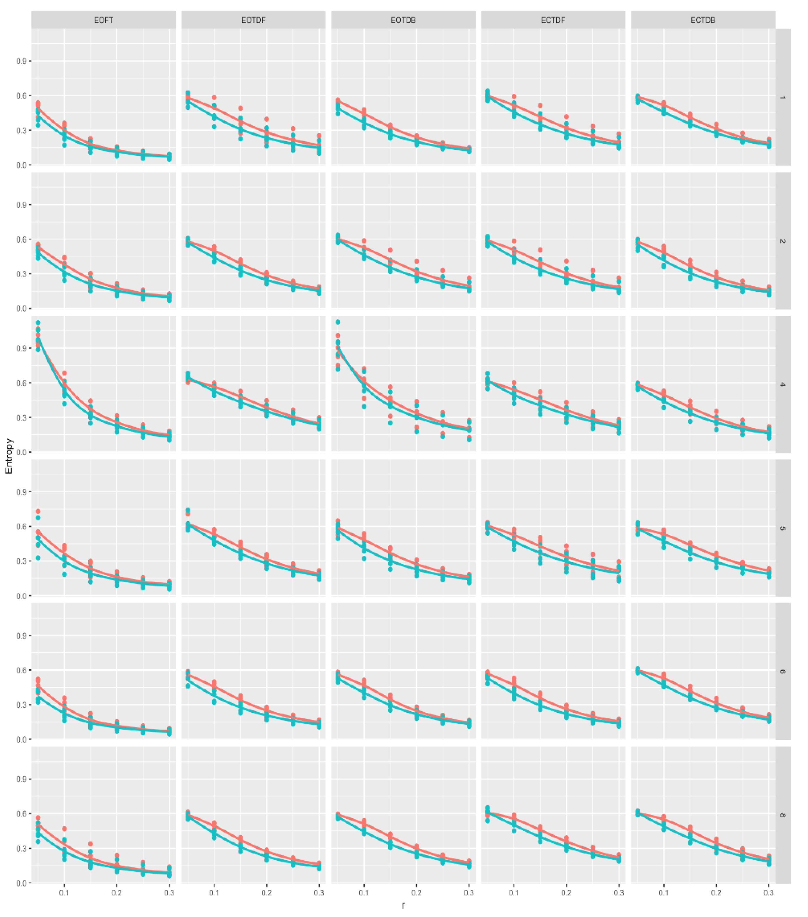
Figure 9). For COP anterior-posterior excursion we found that entropy magnitudes (ApEn and SampEn) in the EOFT condition were larger for
r = 0.05 *SD and 0.10 * SD, and values decreased as
r increased, leveling off after
r = 0.20 * SD. Entropy magnitudes for COP medial-lateral excursion were generally reduced in the EOFT condition compared to the AP excursion data, but decreasing entropy with increasing r mirrored the pattern seen for the AP data. There are no comparable publications related to quiet standing, although Yentes et al. [
16] reported a similar relationship between SampEn and changing
r, but a more variable relationship between ApEn and changing
r. On the other hand, our data demonstrated relative consistency for both ApEn and SampEn with changes in the tolerance window, particularly for
r = 0.20,
r = 0.25, and
r = 0.30 * SD. Based on the good consistency of both ApEn and SampEn using a range of
r’s equal to 0.20, 0.25, and 0.30 * SD we suggest that future research investigating postural sway based on COP time series consider the method we used. Despite the consistency of the ApEn and SampEn values we found, we caution the reader that our choice for determining the tolerance window is limited by any factor, such as data length, nonstationarity of the data, spikes, and outliers, that affect data variance.
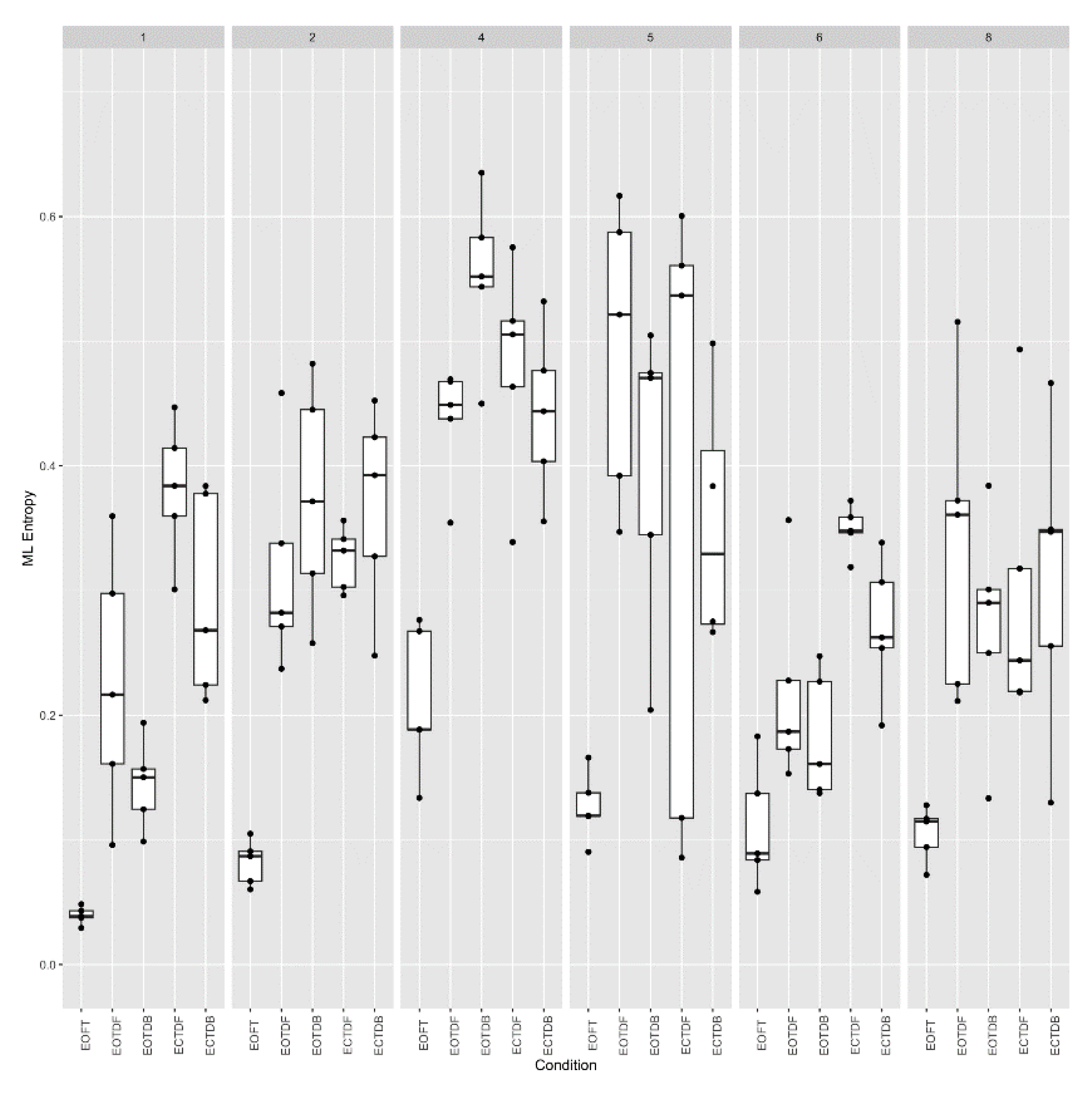
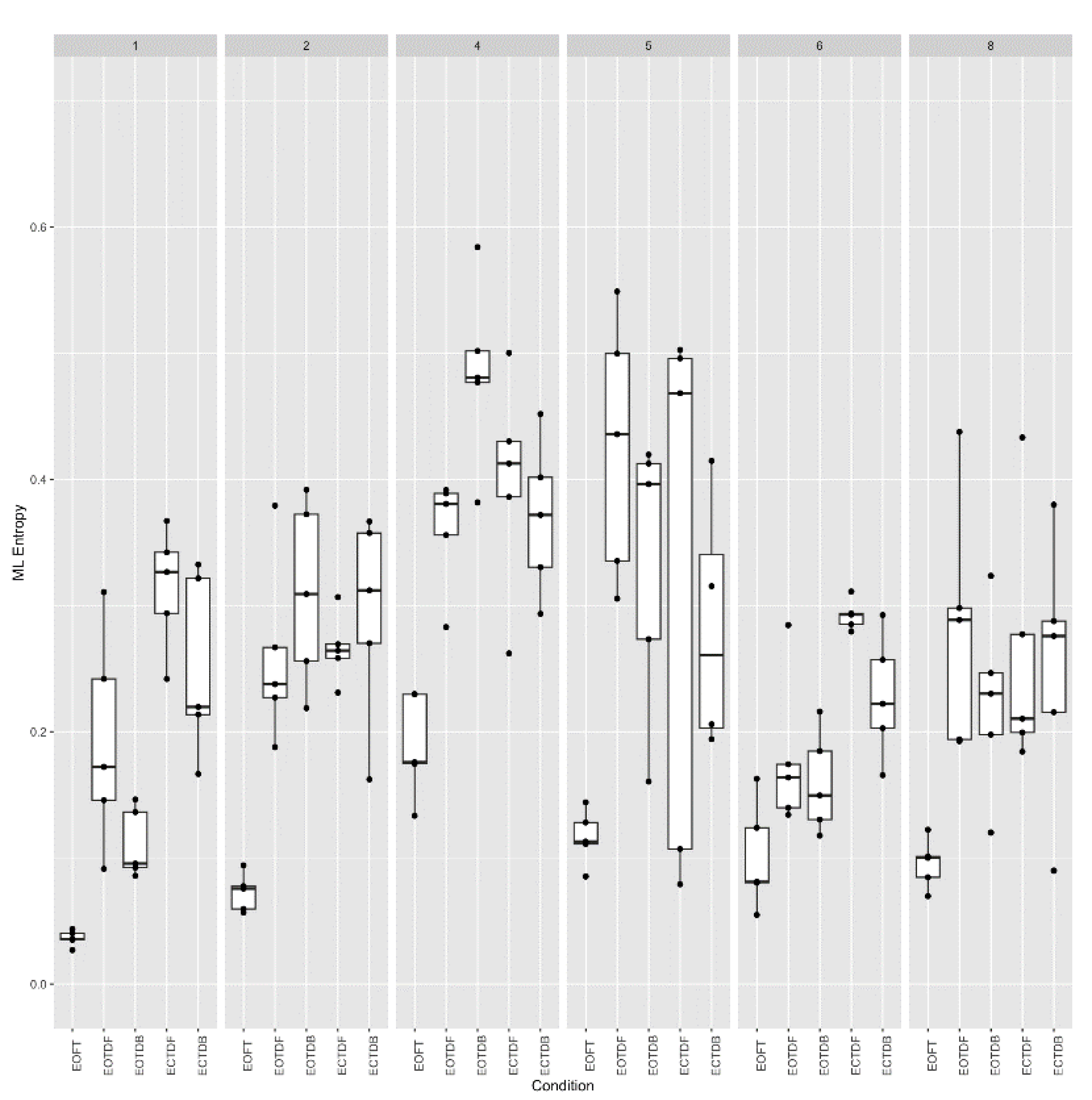
Outliers and spikes were identified in some of our data, particularly for participants #4 and #5 (see
Figure 8,
Figure 9,
Figure 10 and
Figure 11), in the ApEn and SampEn values for
r = 0.05 and
r = 0.1 * SD, likely due to the overly stringent conditions. Molina-Picó et al. [
34] evaluated the impact of abnormal spikes on the interpretation of entropy results in the context of biosignal analysis and suggested removing these results, as they can misrepresent the signal regularity. We believe additional research is needed related to reproducing our findings relative to the entropy values using smaller
r values. For this project, we presented the data using smaller
r values, but are skeptical about their clinical interpretation and meaningfulness.
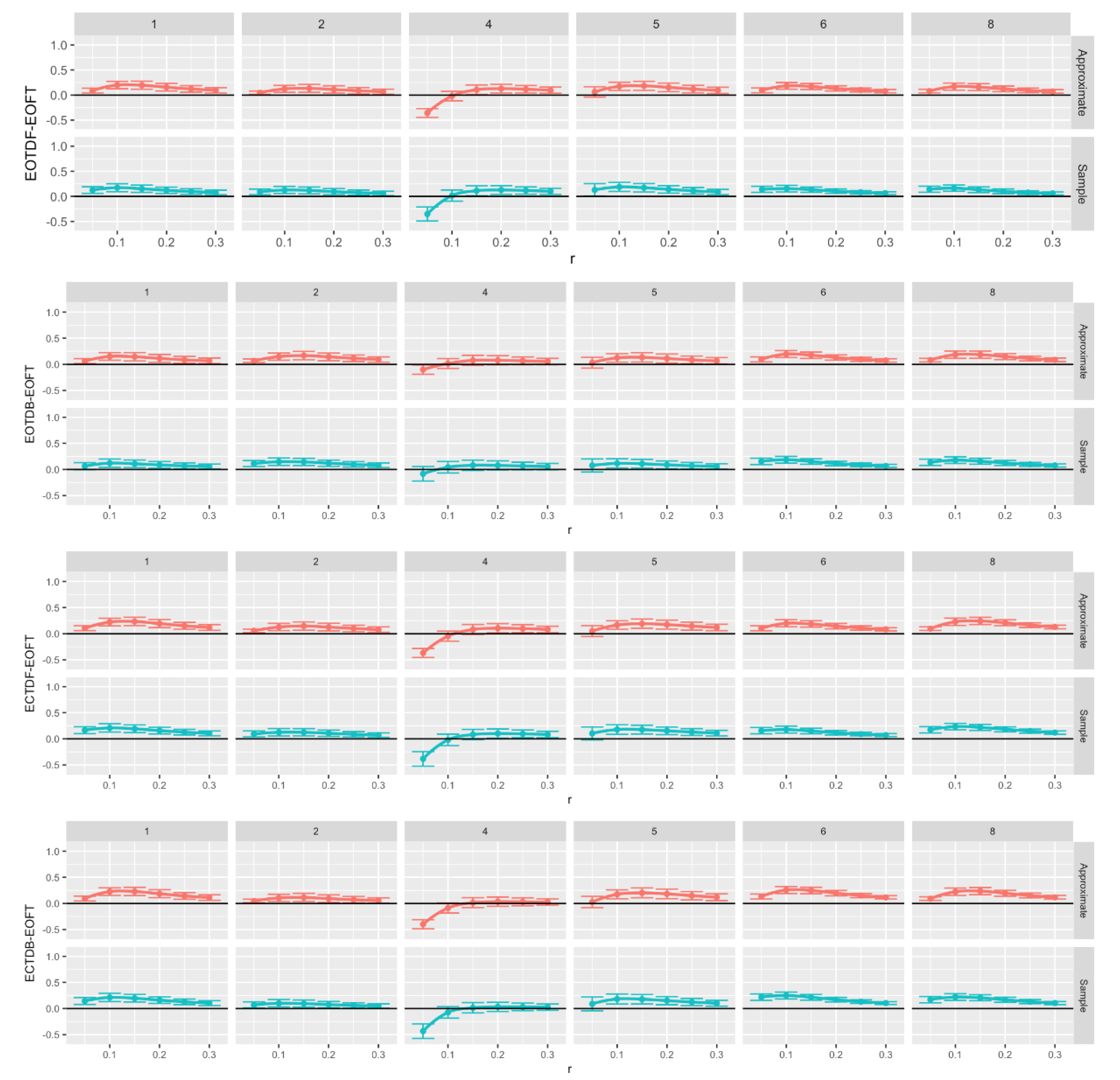
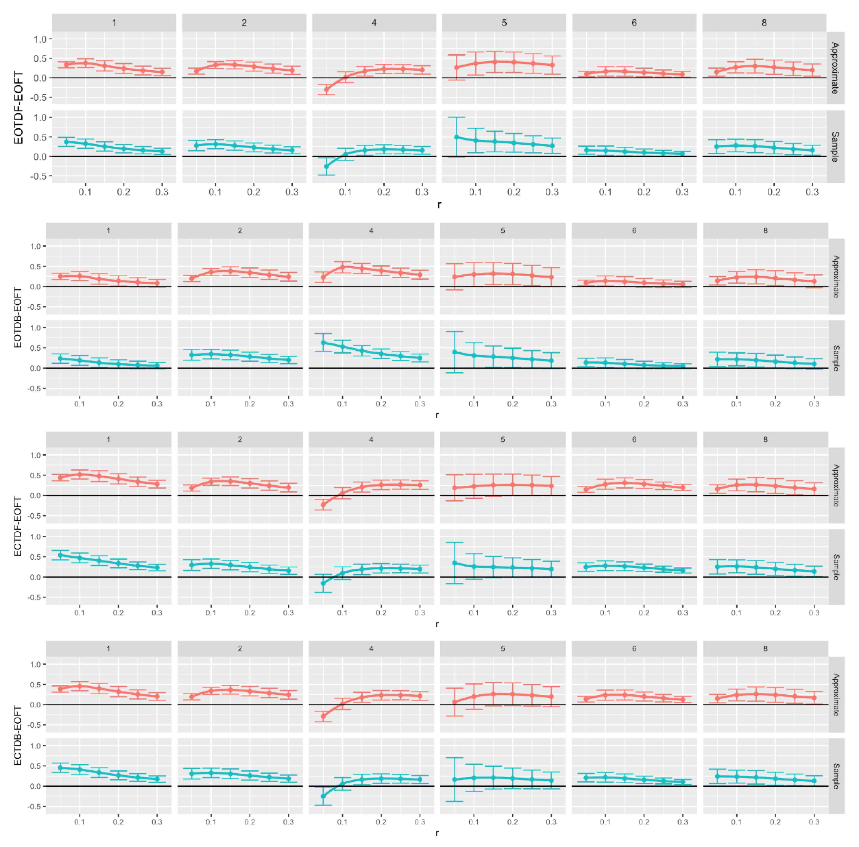
Although we determined ApEn and SampEn for both EOFT and ECFT postures, we chose to use the EOFT posture as a relative baseline for postural stability. An additional purpose of this study was to ascertain whether these two entropies could differentiate signal predictability similarly when comparing a relatively stable quiet standing posture from postures that were more difficult to maintain over a 30-second time frame. Our data showed that ApEn and SampEn values were larger for tandem standing positions whether the eyes were open or closed, and whether the dominant foot (leg) was placed back or forward (
Figure 12 and
Figure 13). Thus, we concluded that the tandem standing positions produced anterior-posterior and medial-lateral COP excursions associated with a system that produced a time series that was more random, less probable and predictable, and one with a greater amount of new information gained from the next data points in the time series [
30]. In another study that assessed quiet standing balance and altering visual conditions, Ramdani et al. [
13] used SampEn to analyze human postural sway. They reported that SampEn distinguished between the eyes open and eyes closed conditions of participants standing on a single force plate. Specifically, in the eyes closed condition, SampEn was lower. Other research results concur with Ramdani’s findings [
49], whereas some reported contradictory results [
52]. One limitation of the present study was that we did not examine whether ApEn and SampEn could distinguish the eyes open from the eyes closed tandem standing postures. Future research should address this.
Since both ApEn and SampEn values were significantly larger with tandem standing postures, compared to the eyes open feet together posture, we wondered which entropic measure was “better”? We are not aware of any previous research that compared ApEn and SampEn from the COP time series for standing balance by altering only the tolerance window. Yentes et al. [
16] investigated the step time series of walking trials and evaluated various combinations of
N, m, and
r. They concluded that SampEn demonstrated excellent relative consistency for long gait data sets when using two different modes of walking, i.e., overground versus treadmill. On the other hand, our results suggest that both ApEn and SampEn demonstrated similar relative consistency.
In addition to reported differences in relative consistency for ApEn and SampEn between Yentes et al. [
16] and our findings, there were also differences when comparing the two entropy value magnitudes. We found that, overall, ApEn magnitudes were larger than SampEn values, whereas Yentes et al. reported that generally mean ApEn values were lower than mean SampEn values in the analysis of step time gait data.
The results of this project may be limited by several methodological decisions. Our sample was limited by convenience and its small size. Additional research is suggested using a larger cross-sectional sample. In addition, will be important to test our methods against different neuropathologies, like post-concussion individuals. As noted in the discussion, there are several suggested methods for determining the tolerance window. It may be useful to compare ApEn and SampEn values using the standard method we used and the other accepted methods, e.g., a fixed tolerance window [
49,
50] and the method suggested by Chon et al. [
47]. Our results may have been influenced by the data resolution of the downsampling technique employed.
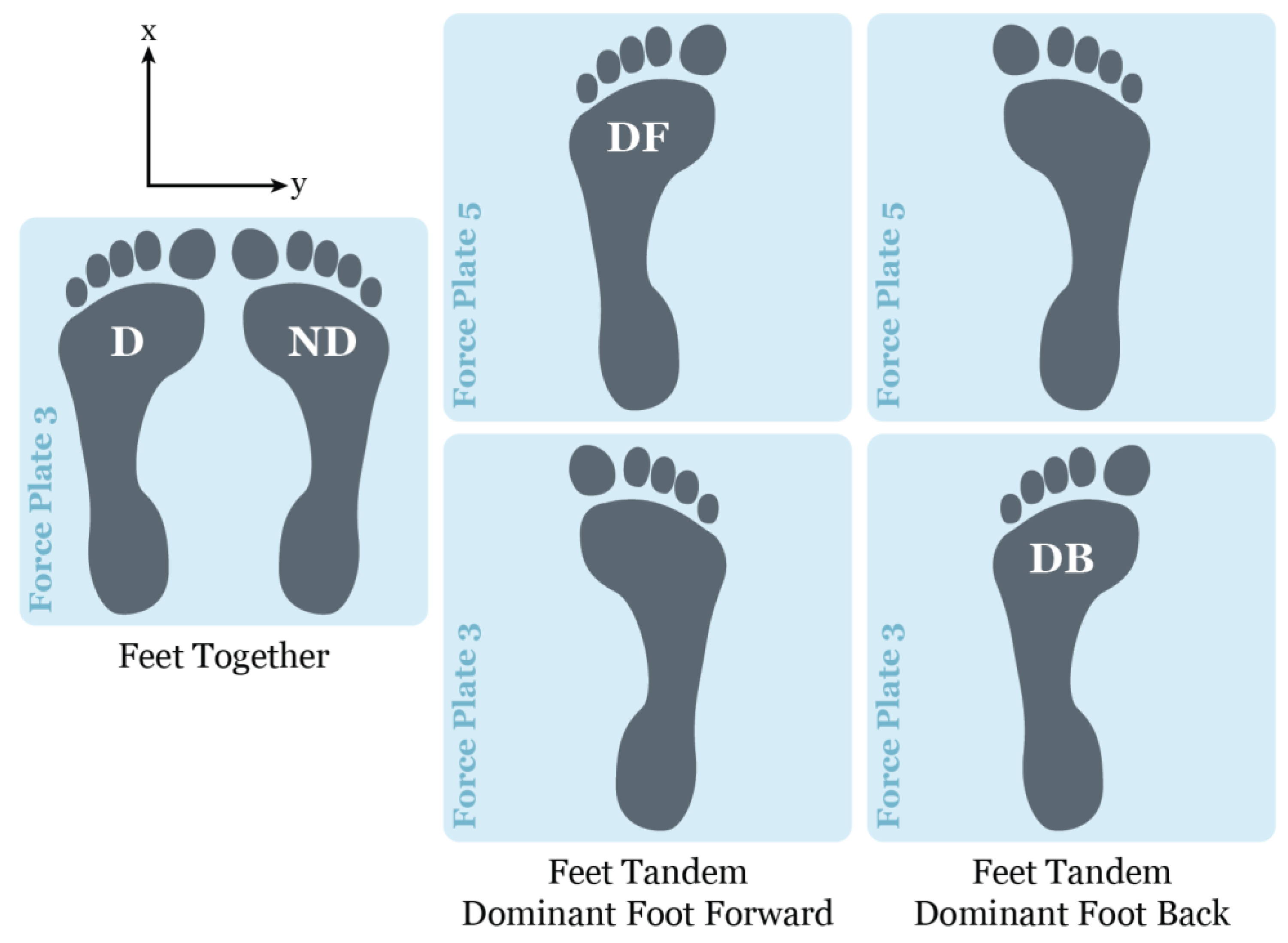
Figure 1.
Force plate foot placement for feet together and feet tandem standing balance conditions, where the x-axis (anterior-posterior (AP) direction) and y-axis (medial-lateral (ML) direction define the center of pressure orientation. Note: D = dominant foot; ND = nondominant foot; DF = dominant foot forward; and DB = dominant foot back [
21,
35].
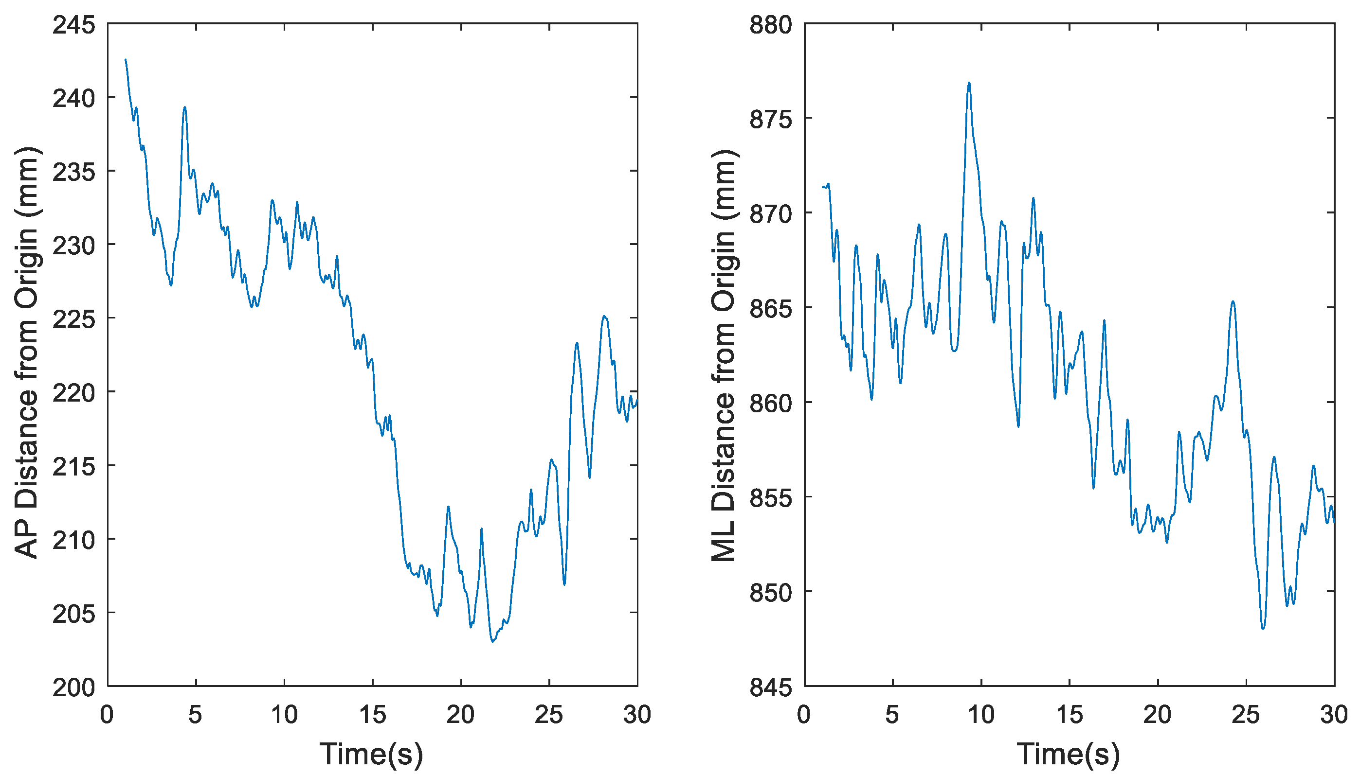
Figure 2.
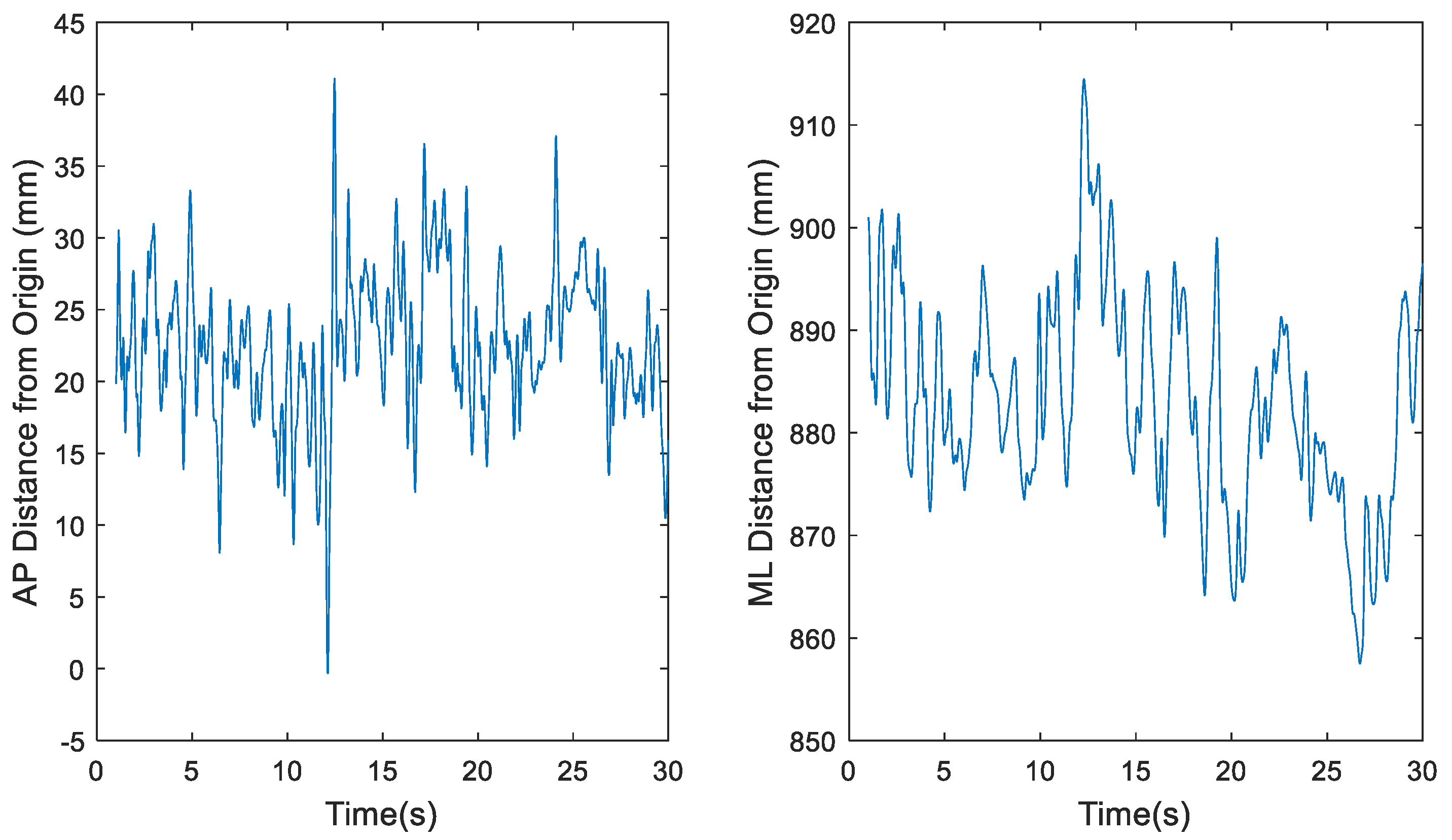
Representative time series for raw center of pressure (COP) data of participant 1 eyes open, feet together (EOFT) Trial 4, where fs = 1200 Hz, in the anterior-posterior (AP) and medial-lateral (ML) directions, respectively.
Figure 2.
Representative time series for raw center of pressure (COP) data of participant 1 eyes open, feet together (EOFT) Trial 4, where fs = 1200 Hz, in the anterior-posterior (AP) and medial-lateral (ML) directions, respectively.
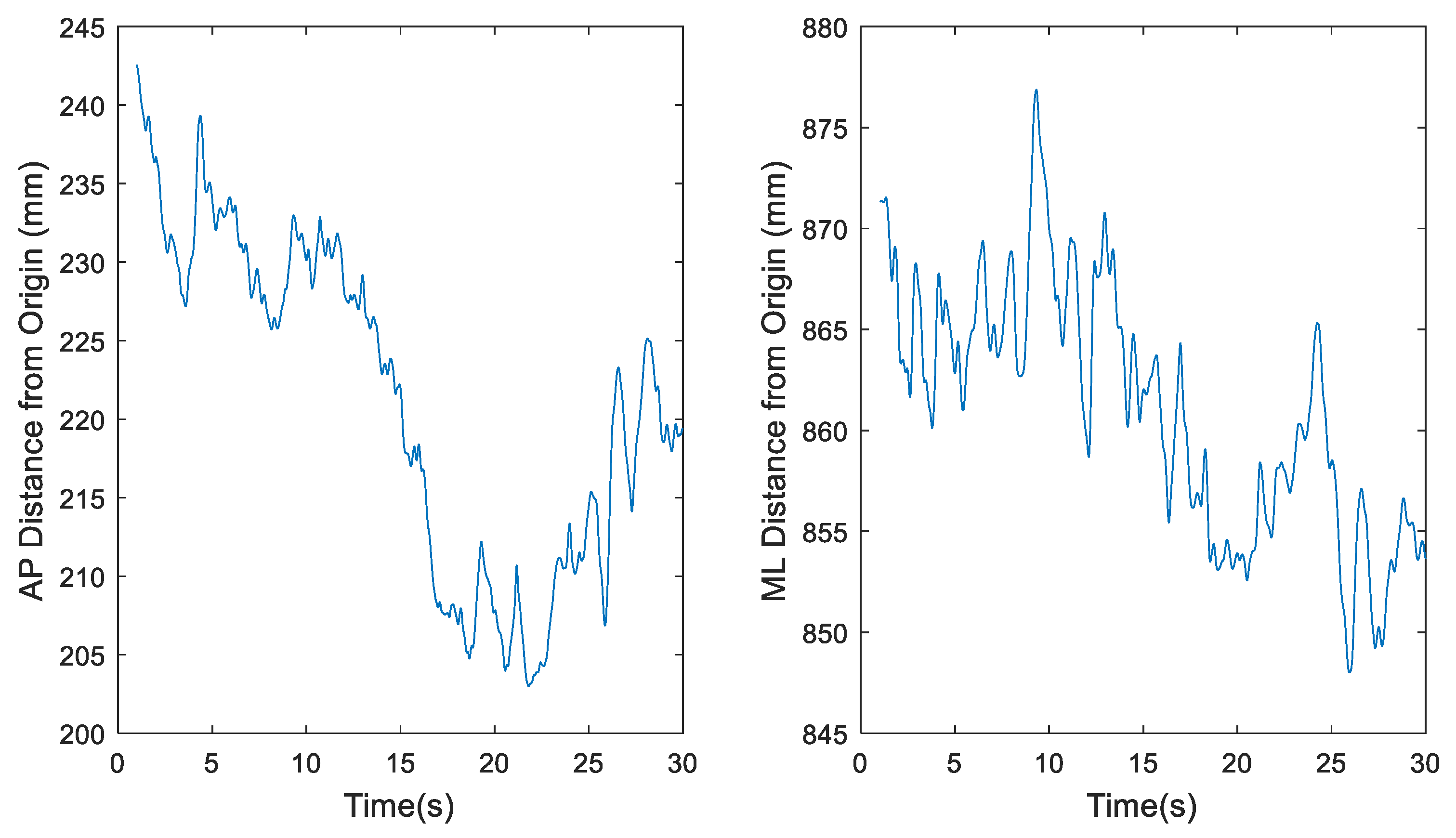
Figure 3.
Representative time series for downsampled center of pressure (COP) data of participant 1 eyes open, feet together (EOFT) Trial 4, where fs = 60 Hz, in the anterior-posterior (AP) and medial-lateral (ML) directions, respectively.
Figure 3.
Representative time series for downsampled center of pressure (COP) data of participant 1 eyes open, feet together (EOFT) Trial 4, where fs = 60 Hz, in the anterior-posterior (AP) and medial-lateral (ML) directions, respectively.
Figure 4.
Representative time series for raw center of pressure (COP) data of participant 1 eyes closed, feet tandem, dominant foot forward (ECTDF) Trial 29, where fs = 1200 Hz, in the anterior-posterior (AP) and medial-lateral (ML) directions, respectively.
Figure 4.
Representative time series for raw center of pressure (COP) data of participant 1 eyes closed, feet tandem, dominant foot forward (ECTDF) Trial 29, where fs = 1200 Hz, in the anterior-posterior (AP) and medial-lateral (ML) directions, respectively.
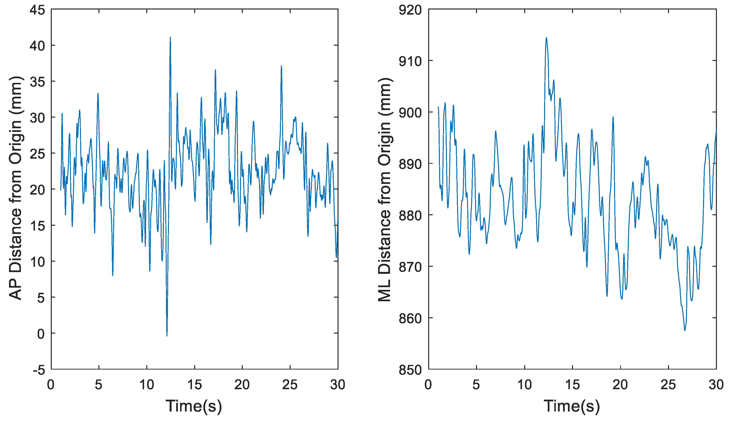
Figure 5.
Representative time series for the downsampled center of pressure (COP) data of participant 1 eyes closed, feet tandem, dominant foot forward (ECTDF) Trial 29, where fs = 60 Hz, in the anterior-posterior (AP) and medial-lateral (ML) directions, respectively.
Figure 5.
Representative time series for the downsampled center of pressure (COP) data of participant 1 eyes closed, feet tandem, dominant foot forward (ECTDF) Trial 29, where fs = 60 Hz, in the anterior-posterior (AP) and medial-lateral (ML) directions, respectively.
Figure 6.
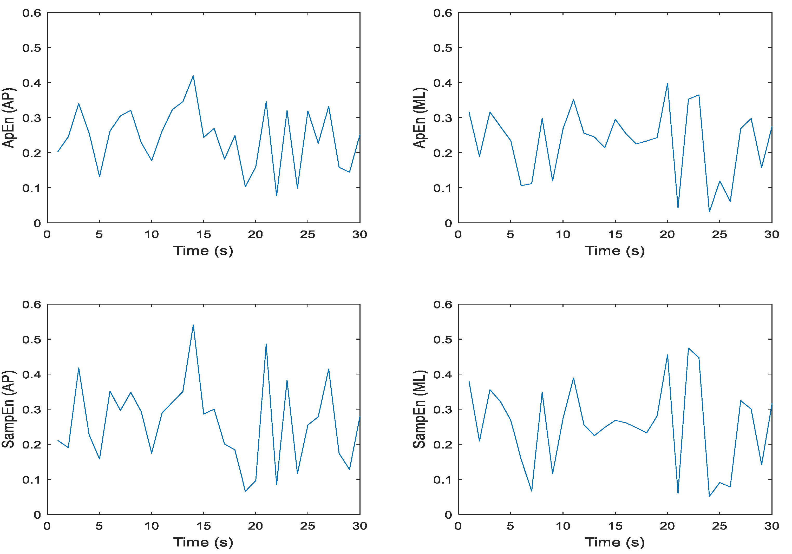
Representative time series for ApEn and SampEn calculated every second for 30 seconds for participant 1 eyes open, feet together (EOFT), Trial 03 COP data; where N = 60 datapoints, m = 2, and r = 0.2 * SD; in the anterior-posterior (AP) and medial-lateral (ML) directions, respectively.
Figure 6.
Representative time series for ApEn and SampEn calculated every second for 30 seconds for participant 1 eyes open, feet together (EOFT), Trial 03 COP data; where N = 60 datapoints, m = 2, and r = 0.2 * SD; in the anterior-posterior (AP) and medial-lateral (ML) directions, respectively.
Figure 7.
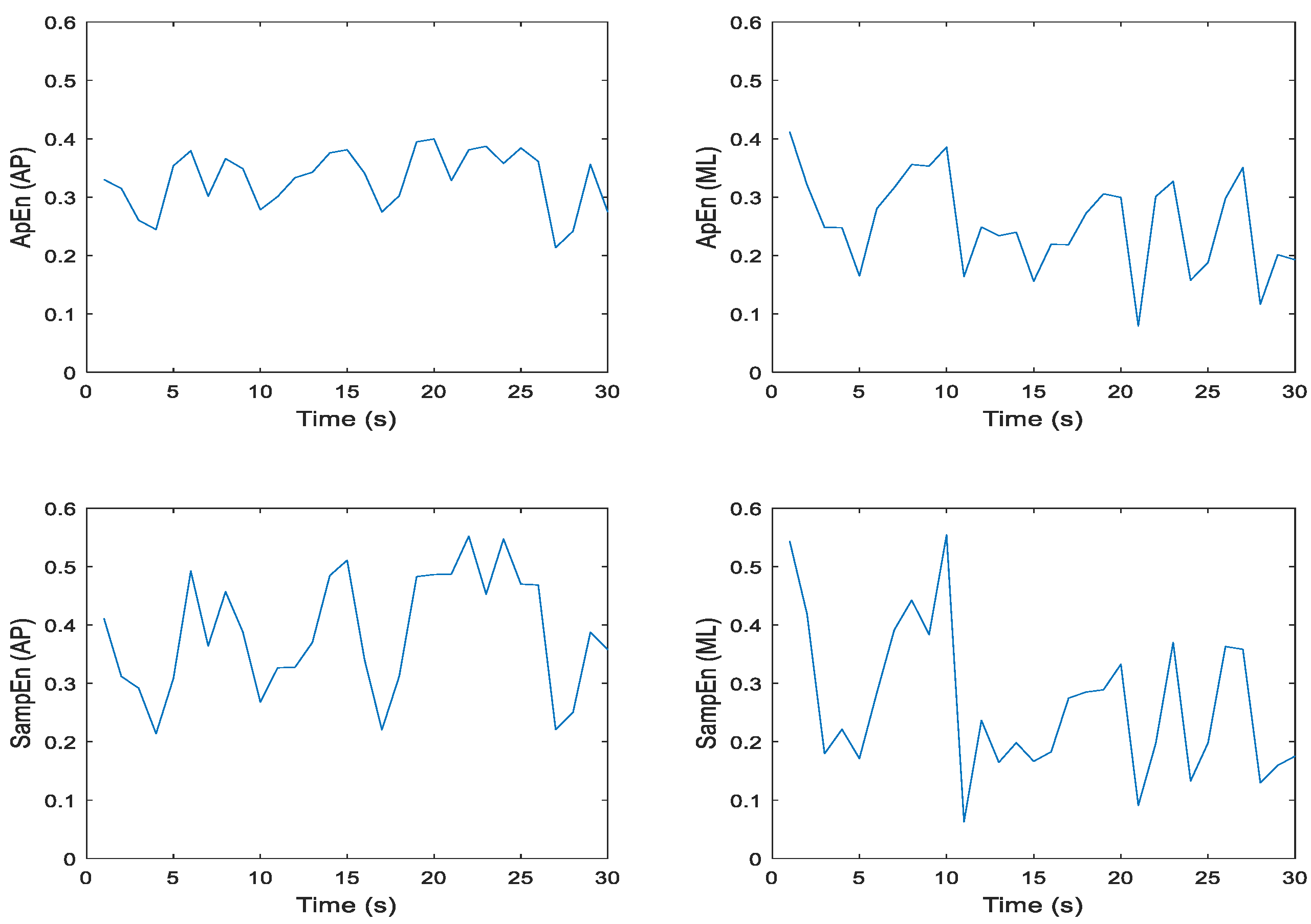
Representative time series for ApEn and SampEn calculated every second for 30 seconds of participant 1 eyes closed, feet tandem, dominant foot back (ECTDB), Trial 19 COP data; where N = 60 datapoints, m = 2, and r = 0.2 * SD; in the anterior-posterior (AP) and medial-lateral (ML) directions, respectively.
Figure 8.
Anterior-posterior (AP) direction approximate (red) and sample (blue) entropy values (vertical axis) versus six different tolerance windows (horizontal axis), i.e., r, while standing in five different postures, i.e., eyes open feet together (EOFT), etc., for each participant. Note that 12 r and Method, i.e., ApEn or SampEn, quantities were derived from each COP time series. There were five time series for each cell giving 60 graphed points in each cell. Loess curves are provided to help visualize the relationship between r and entropy values for each method in each cell.
Figure 9.
Medial-lateral (ML) direction approximate (red) and sample (blue) entropy values (vertical axis) versus six different tolerance windows (horizontal axis), i.e., r, while standing in five different postures, i.e., eyes open feet together (EOFT), etc., for each participant. Note that 12 r and Method, i.e., ApEn or SampEn, quantities were derived from each COP time series. There were five time series for each cell giving 60 graphed points in each cell. Loess curves are provided to help visualize the relationship between r and entropy values for each method in each cell.
Figure 10.
Approximate entropy (vertical axis) (m = 2, r = 0.25 * SD) across six participants for all standing postural test conditions (horizontal axis). Data collected consisted of five trials for each participant at each stance condition. Each boxplot is derived from the five calculated entropy values for each condition for each participant (30 boxplots).
Figure 11.
Sample entropy (vertical axis) (m =2, r = 0.25 * SD) across six participants for all standing postural test conditions (horizontal axis). Data collected consisted of five trials for each participant at each stance condition. Each boxplot is derived from the five calculated entropy values for each condition for each participant (30 boxplots).
Figure 12.
Comparison of Approximate (red) and sample (blue) entropy values across standing postural conditions for the center of pressure data in the anterior-posterior (AP) direction for each participant. Note that all F-tests, except six, had p < 0.05. What is graphed are Dunnet’s 95% confidence intervals. Loess curves through the confidence interval centers are included to aid visualization. Significant intervals can be found above the black (zero) horizontal line. Comparison pairs along the vertical axis, with r values along the horizontal axis.
Figure 13.
Comparison of Approximate (red) and sample (blue) entropy values across standing postural conditions for the center of pressure data in the medial-lateral (ML) direction for each participant. Note that all F-tests, except six, had p < 0.05. What is graphed are Dunnet’s 95% confidence intervals. Loess curves through the confidence interval centers are included to aid visualization Significant intervals can be found above the black (zero) horizontal line. Comparison pairs along the vertical axis, with r values along the horizontal axis.
Figure 14.
Histograms, i.e., count (vertical axis) of the difference between SampEn and ApEn, i.e., Sample-Approximate (horizontal axis). Values to the left of the vertical black line indicate that ApEn was larger and values to the right of the vertical black line indicate that SampEn was larger.
Figure 14.
Histograms, i.e., count (vertical axis) of the difference between SampEn and ApEn, i.e., Sample-Approximate (horizontal axis). Values to the left of the vertical black line indicate that ApEn was larger and values to the right of the vertical black line indicate that SampEn was larger.
Table 1.
Quiet Standing Balance Test Conditions.
Table 1.
Quiet Standing Balance Test Conditions.
| Balance Condition |
Description |
| EOFT |
Eyes Open, Feet Together |
| ECFT |
Eyes Closed, Feet Together |
| EOTanDF |
Eyes Open, Feet Tandem, Dominant Foot Forward |
| ECTanDF |
Eyes Closed, Feet Tandem, Dominant Foot Forward |
| EOTanDB |
Eyes Open, Feet Tandem, Dominant Foot Back |
| ECTanDB |
Eyes Closed, Feet Tandem, Dominant Foot Forward |
