In pavement performance models, the state space represents different pavement conditions measured by composite condition indices (e.g., pavement condition index (PCI)), individual distresses (e.g., cracking), or remaining service lives [
6]. The condition state vector is a list of probability distributions corresponding to the pertinent state space;
=
; where
is the condition state vector at time
any
and
. Markov models estimate the future pavement condition
based on the current pavement condition
) according to the memoryless property of Markov process and the transition probabilities of pavement deterioration and improvement
;
=.
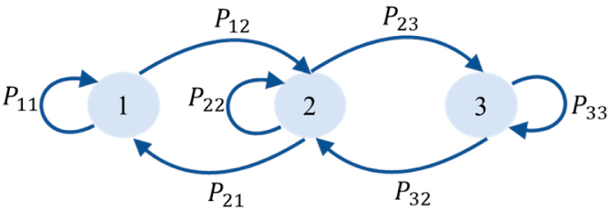
Pavement condition bounces across three phases: (1) stays at its current state
, (2) transits to lower states
, or (3) transits to upper states
, when maintenance or rehabilitation treatment is implemented. The condition state vector is comprised of a number of condition states defined by their probability distributions. The number of condition states depends on data availability [
9], and it needs to be chosen prudently to capture the entire pavement condition over its lifespan [
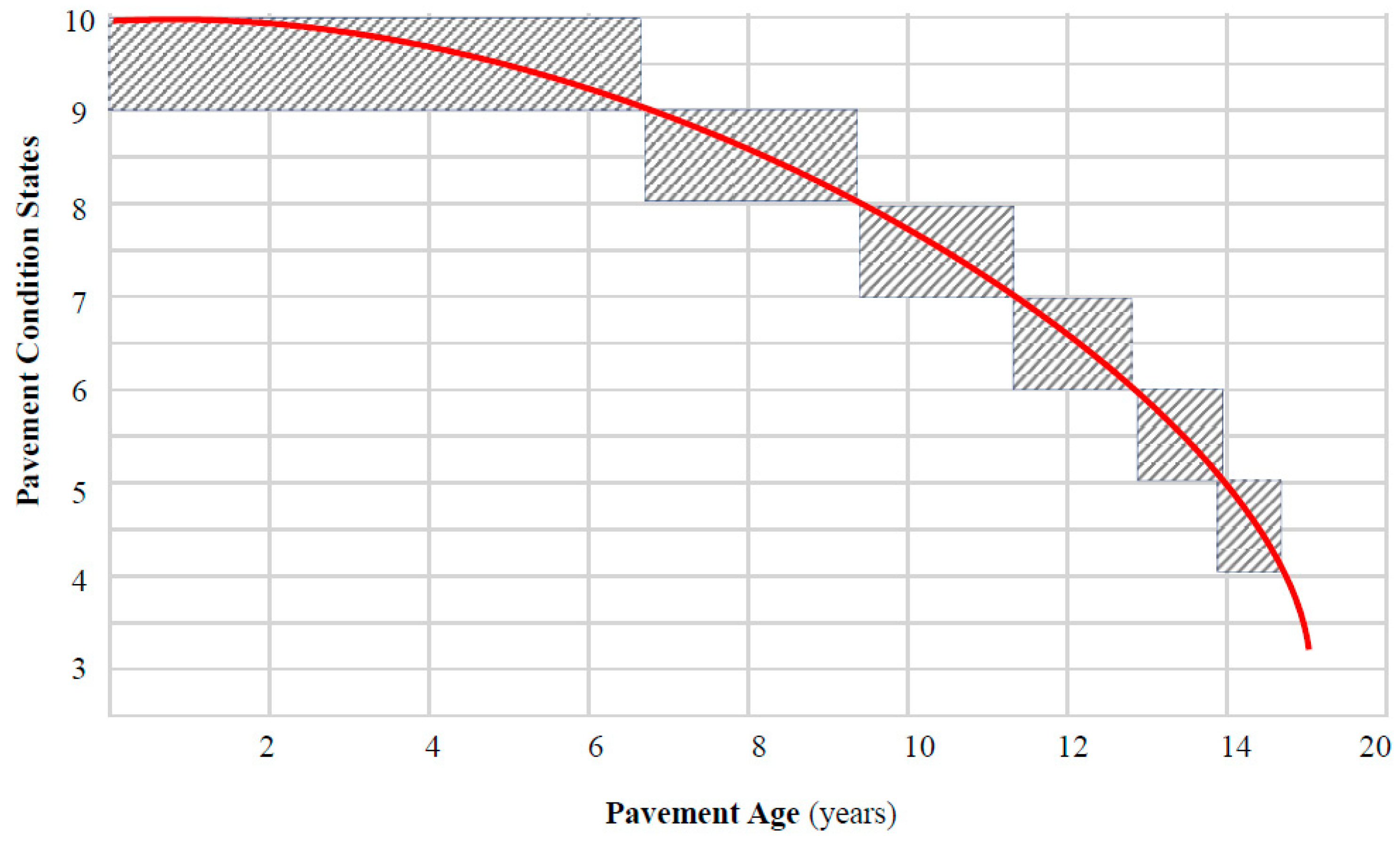
6]. In pavement performance models, typically 10 condition states (from 1 to 10) are assumed; where state 1 represents the best condition, and state 10 represents the worst condition. However, past research assumed different numbers of pavement condition states such as 20 states [
10] and four states [
6]. The probability distribution of each condition state is calculated as the percentage of the number of pavement sections or the number of pavement lane-miles that lies within each state to the total size of pavement network.
The common assumptions of Markov chain models for pavement condition prediction include pavement deterioration is a discrete process, whereas it is continuous in nature. The duty cycle is one year because most highway agencies inspect their pavements annually. Pavement condition states can only move to one state lower every duty cycle. In other words, in the square TPM matrix, andare the only existent probabilities in each row of the matrix; where is the state number, and. The effect of the maintenance and rehabilitation treatments is not considered in estimating pavement transition probabilities, i.e., . The last state is an absorbing state, i.e.,, because it is the worst condition state pavements can occupy.
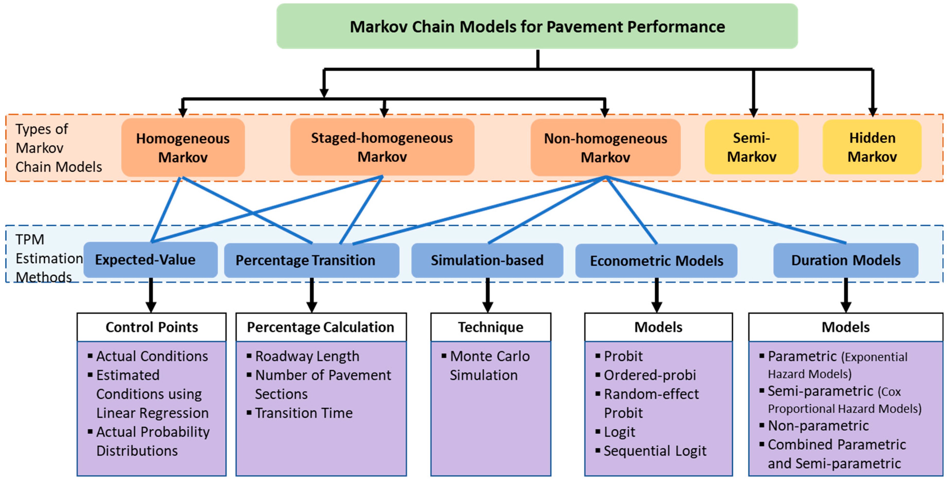
Homogeneous Markov Models
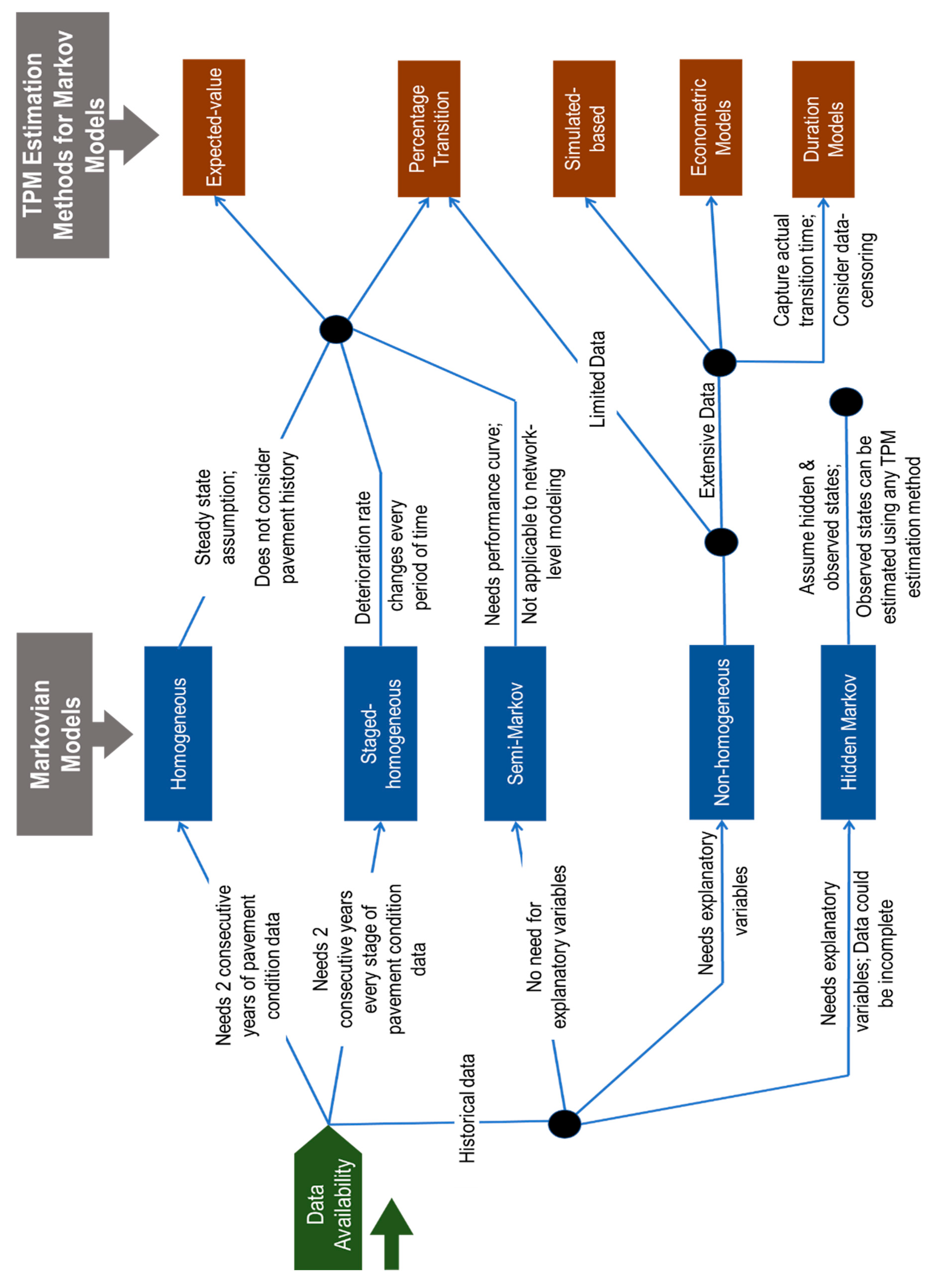
These models are time-independent, do not require large amounts of historical data, and are computationally simpler for pavement condition prediction. The data needed for these models is the pavement condition observations of two successive transitions. The future pavement condition after a period of time is calculated by multiplying the current probability distributions () by the TPM () raised to the power;.
The TPM of homogeneous Markov models is estimated using the expected-value or percentage transition methods. The expected-value method estimatesby minimizing the difference between the predicted pavement condition using Markov models and predetermined control points. These control points could be: (1) the actual pavement condition, (2) the predicted pavement condition using simple linear regression analysis, or (3) the actual probability distributions of pavement condition. The percentage transition method estimatesas the percentage of the amount of pavements (number of pavement sections, total length of pavement sections, or total remaining service lives of pavement sections) that have moved from state to state during the time to the amount of pavements that was originally in state .
[
20] used the expected-value method to derive TPMs for homogeneous Markov models to predict pavement cracking, raveling, roughness, and rutting. To estimate the TPM, they minimized the difference between the models’ predictions and each control point. Ten condition states and 1-year duty cycle were assumed for the Markovian model structure. Different pavement performance patterns were assumed, and then pavement condition data was generated for 20 years. Pavement condition was predicted using the minimization with respect to each type of control points and then compared with the actual observations. For the control points 1 and 2, the predicted pavement conditions were found to be different from the actual observations, but for the third type of control points, the predicted and actual probability distributions were found to be similar. Hence, the excepted-value method is considered of high reliability in estimating pavement TPM when the third type of control points is used. [
21] derived TPMs for homogeneous Markovian models using the percentage transition method to predict pavement cracking and roughness in Arizona. Pavement sections were categorized into various groups based on traffic volume and weather condition to account for the variation in the data of pavement sections. [
21] found that the developed pavement performance curves using the percentage transition method match the actual performance curves. [
19] developed homogeneous Markov models to predict pavement distress ratings and PCR in the state of Ohio. Ten condition states and 1-year duty cycle were assumed for the Markov model structure. The transition probabilities were estimated using the percentage transition method and the methodology introduced by [
21]. Pavements were grouped based on their respective traffic volume, weather condition, and treatment type. The estimated TPM was found to be overestimated during the latter ages of pavement, and so the researchers used the statistical imputation to overcome this overestimation.
[
16] and [
22] estimated the TPM for homogeneous Markovian models to optimize pavement rehabilitation treatments and predict pavement distress rating (DR) in Palestine. Ten condition states and 1-year duty cycle were assumed for the Markovian models’ structure. The TPM was estimated as the percentage of the number of remaining pavement sections in each state at the end of the duty cycle to the total number of sections at the beginning of the duty cycle. [
17] found that pavement deterioration rates do not change significantly during a period of 5 or 6 years, and thus [
16] assumed an analysis period of 5 years for their model. [
22] investigated the sensitivity of the TPM to pavement section lengths 10, 30, 50 and 100m, and he concluded that the transition probabilities become more unstable when pavement section length increases. As a result, he recommended using shorter pavement sections to avoid instability in TPM values.
[
23] developed homogeneous Markov models to predict pavement present serviceability index (PSI). He estimated the TPM as the ratio between the actual transition time that each state takes to move to the next state and the duty cycle. He assumed five condition states and one and two years for the duty cycle. The transition time was interpolated from a deterministic pavement performance curve that represents the relation between pavement PSI and respective equivalent single axle loads (ESALs) using the AASHTO's design methodology [
1]. The estimated transition probabilities were found to be consistent with the engineering intuition.
Table 1 shows the key studies that used the expected-value and the percentage transition methods to estimate TPMs for homogenous Markov models for pavements.
Although the homogenous Markov models are computationally easy, they suffer from several drawbacks. The results of homogeneous Markov models can be questionable because of their stationary assumption [
4]. This assumption ignores the change in pavement deterioration rate due to the increase in traffic loading and the degradation of pavement structural capacity [
15]. Additionally, the homogeneous Markovian models do not account for the impact of the exogenous variables such as traffic loads and environmental conditions. To overcome this limitation, pavement sections can be segmented based on pavement attributes such as pavement age, traffic loading, and climate severity. However, the pavement section segmentation decreases the sample size which in turn lowers the accuracy of Markovian models. Homogeneous Markov models could yield an overestimation of pavement condition over the entire lifetime of pavement [
38] or its latter ages [
19]. This overestimation could lead to insufficient M&R actions during pavement life. Statistical imputation techniques were recommended by [
19] to avoid this expected overestimation.
The expected-value and transition percentage methods are typically used to derive constant TPMs for the homogeneous Markov models of pavement condition prediction. These methods require two consecutive transitions of pavement conditions, which is insufficient to capture the historical behavior of pavements. To overcome this limitation, [
20] suggested calculating the average transition probabilities for more than one duty cycle. [
32] concluded that the expected-value method is more accurate than the percentage transition in estimating the TPM for modeling timber bridges’ elements. In the expected-value method, the methodology of minimizing the difference between the estimated pavement condition using simple linear regression and using Markov models is unreliable since the relationship between pavement condition and pavement age is non-linear, and pavement age is not the only variable influences pavement condition.
Staged-Homogeneous Markov Models
[
17] introduced this type of models to overcome the limitation of data unavailability when developing a non-homogeneous Markov model. Staged-homogeneous Markov models involve dividing the analysis period into zones, each of 5 or 6 years at maximum. Pavement sections are sorted and grouped based on their ages. Homogeneous TPMs are established for every zone. The future condition of pavement section at any time
is calculated by multiplying the current probability distributions of this section by the TPM of every zone until the time
, i.e.,
; where
is the TPM of the first zone raised to power
, and
is the zone size in years;
is the TPM of the zone that includes the time
, and
is the number of zones until the zone that includes
. In the staged-homogeneous Markov models the TPM is estimated using the expected-value or percentage transition methods.
[
17] developed a staged-homogeneous Markov model to predict pavement PCI using data from the PAVER database. They assumed 10 condition states with 1-year duty cycle for the Markov model structure. The zone size was assumed to be 6 years. The TPM was estimated using the expected-value method by minimizing the difference between the actual and predicted pavement condition. The developed model was validated by comparing its predictions with the actual observations and with the predictions from a previous homogeneous Markov model that was developed by Keane and Wu (1985) in collaboration with the U.S. Army Construction Engineering Research Laboratory (USA-CERL). The results showed that the staged-homogeneous Markov model of [
17] outperforms its homogeneous counterpart of Keane and Wu (1985). [
15] presented staged-homogeneous Markov models to predict pavement deterioration rate (DR) using data spanning from 1998 to 2015 for a major urban arterial road in Palestine. Two models were built: three-year and five-year staged-homogeneous Markov models. The TPMs were estimated using the percentage transition method with the transition probability equals the proportion of the number of pavement sections that transits from one state to another. The TPM was assumed to change by a constant
C every stage/zone (3 or 5 years) in both models. The constant C was assumed to take on values greater than 1, and its value was exactly determined by minimizing the difference between the actual and predicted transition probabilities/DRs. Both models of [
15] were found to be statistically reliable in predicting pavement condition. However, the three-year staged-homogeneous Markov model was found to be superior to the other model with respect to the sum square errors (SSE).
Table 2 summarizes the methods of estimating the TPM in the expected-value and percentage transition methods for the staged-homogeneous Markov models, and key studies that used these methods for pavement performance modeling.
The staged-homogeneous Markov models have two advantages. First, they are more reliable than the homogeneous Markov models in pavement condition prediction because they account for the non-stationary process of pavement deterioration. Second, they require relatively limited amounts of data. However, since the staged-homogeneous Markov models use the expected-value and percentage transition methods to estimate TPMs, they suffer from the limitations of these TPMs’ estimation methods (discussed earlier). Unlike the staged-homogeneous Markov models found in the literature and because pavement deterioration rate varies over time, the analysis period should be divided into unequal zones based on pavement performance curve and its respective rate of deterioration, not into constant zones.
Non-Homogeneous Markov Models
These models are time-dependent and consider the non-stationary property of pavement deterioration process. These models account for the uncertainty inherently attributed to explanatory variables such as traffic loads and weather conditions [
4,
13,
15,
39]. Although non-homogeneous Markov models fit realistically the random behavior of pavement condition over time, they have not been adopted widely in pavement performance modeling because they require extensive computation and large amounts of data. The future condition of pavement at any time
is calculated by multiplying the current probability distributions of this pavement by the TPM of every duty cycle until the time
, i.e.,
. In non-homogeneous Markov models, the TPM is estimated using one of the following methods: percentage transition, simulation-based, econometric models or duration models.
[
40] developed a non-homogeneous Markov model to predict pavement DR in Palestine. Ten condition states and 1-year duty cycle were assumed for the Markovian model structure. He used the percentage transition method to estimate the TPM of the first duty cycle. The remaining TPMs were calculated by multiplying the TPM of the first duty cycle by the two factors: traffic loads and pavement structure number. The developed models yielded transition probabilities comparable with the actual data, which ascertains that the change in pavement deterioration rate due to traffic loading should be considered when modeling pavement performance. Furthermore, the TPM can be estimated using the simulation-based method in which transition probabilities are expressed in terms of the percentiles of pavement condition states. [
39] and [
41] used this method to develop non-homogeneous Markov models to predict pavement condition. The pavement deterioration formula developed in the model of Ontario Pavement Analysis of Cost (2000) was employed, and the impact of the ensuing explanatory variables was included: material modulus and thickness of each pavement layer, subgrade modulus, annual average daily traffic (AADT), traffic growth rate, truck percentage, number of traffic lanes in each direction, and ESALs. Using Monte Carlo simulation, the transition probabilities of pavement condition were estimated assuming that the studied variables follow the standard normal distribution. The researchers further checked the sensitivity of the transition probabilities to the independent variables considered in their study, and they found that pavement transition probabilities are significantly sensitive to traffic growth rate, subgrade strength and pavement layer thickness.
The econometric models are recommended for TPM estimation to reflect the historical behavior of pavement condition based on large amounts of historical data. These models associate pavement deterioration with the influential pertinent explanatory variables. Also, they yield pavement condition predictions that are more accurate than that obtained from the abovementioned methods, percentage transition and simulation-based [
42,
43,
44]. The key econometric models that are used in Markovian pavement performance models include Probit, Logit and Ordered-Probit. Probit and Logit models are employed to statistically model pavement condition states as discrete variables. They are grouped into binary and multinomial models based on the number of outcomes of the model. These models assume a latent continuous dependent variable (
) that takes values from
to
, and correlates with an explanatory variables vector (
). The probability of selecting a specific choice or for the outcome to be a specific value depends on the estimated
for all choices or for all expected values. Equation 2 shows the estimation of the Probit or Logit models; where
is the probability of choice
,
is the total number of choices,
is the number of observations,
is the model parameter, and
is the error term.
In Probit models, the error term follows the standard normal distribution (
), whereas, in Logit models, it follows the logistic distribution. The maximum likelihood estimation (MLE) method is used to estimate models’ parameters (
by maximizing the log-likelihood function that is illustrated in Equations 3 and 4 for Probit and Logit models, respectively.
where
is the value of the choice
. [
44] developed a non-homogeneous Markov model to predict pavement cracking rate using Logit models to estimate the TPM. Pavement condition data were retrieved from the state of Florida during the period from 1986 to 2003. The pavement age, ESALs, crack index (CI) and a number of rehabilitation cycles were found to be statistically significant in estimating pavement TPMs. The researchers set the pavement data of 2003 aside to build a homogeneous Markov model, and then compare its results with that of the non-homogeneous Markov model. The values of the validation measures: average absolute error (AAE), root mean square error (
) and coefficient of determination (
), demonstrated that the superiority of the non-homogeneous Markov model to the homogeneous Markov model. The study conducted by [
44] assures that pavement condition propagates due to exogenous variables that should be taken into account when developing Markovian prediction models for pavements. [
45] developed an artificial neural networks (ANNs) model to predict pavement CI. The research team compared the results of the ANNs model with that of their non-homogeneous Markov model of [
44]. Based on the values of the same validation measures they used in 2005 with respect to both models, they found that both models have a similar performance for a single-year prediction, but the non-homogeneous Markov model was found to be more accurate than the ANNs for multiple-year predictions.
Ordered-Probit models estimate discrete and ordered dependent variables when the order matters. Equations 5 shows the estimation of Ordered-Probit models.
where
is the choice of
observations,
is the choice value (
),
is the cumulative distribution function, and
is the order of the choice
. The MLE method is used to estimate the model’s parameters (
. [
4] developed ordered-Probit and sequential Logit models to estimate the TPM for pavement PSI prediction. The sequential Logit model is a series of independent binary Logit models. Unlike ordered-Probit models, sequential Logit models account for the dependency between condition states. Pavement structure and environment relevant variables and traffic loading were considered in these models. Data from the AASHO Road Test was employed for models’ validation. These models were compared with prior three models namely, the non-homogeneous and homogenous Markov models of [
17,
21], respectively, and the duration model [
46]. The ordered-Probit and sequential Logit models were found to be reliable in the prediction of pavement PSI, and more accurate than the prior three models.
Duration models assume that the transition probability of pavement condition is the probability distribution of the time elapsed until pavement changes its condition state. Duration models are effective in estimating the TPMs if relevant data are available for more than 10 years. Also, they account for censored data that is inherently associated with infrastructure data collection [
7]. In the duration models, the data is considered either left-censored, right-censored or interval censored if the duration of leaving a given state is less than a certain value, greater than a certain value or on an interval between two values, respectively. The estimation of pavement transition probabilities using duration models is presented in Equations 6 and 7 based on the study of [
47].
where
is the transition probability from state 1 to state 0 during the time
conditional on the observed state 1 at time
,
is the cumulative distribution function of the duration random variable
,
is the survivor probability. When
approaches Zero the transition probability is called hazard rate. The hazard rate is estimated using parametric, semi-parametric or nonparametric models. In parametric models, the hazard rate follows a pre-specified distribution such as the normal or exponential distribution, which is a limitation of these models [
47]. Semiparametric models relax the limitation of the parametric models and determine the distribution of the hazard rate based on the actual data. Unlike parametric models, Semiparametric models relate the hazard rate to its pertinent exogenous variables. Nonparametric models neither assume distribution function nor derive a specific relation between the hazard rate and its exogenous variables [
7], but it mainly depends on the training dataset. [
13] developed condition prediction models for pavement IRI, rutting and cracking. For the estimation of pavement TPMs, they implemented the duration models to account for the irregularities in pavement inspection periods. Pavement condition was discretized to five condition states. Four hazard models following the exponential distribution were developed to calculate the transition probabilities of states 1, 2, 3 and 4. The ESALs and the structural number (SN) variables were included in the hazard models. Data from a national highway in Korea was used for models’ validation. The results showed that the predicted transition probabilities fit the actual observations.
Table 3 shows a summary of the TPM estimation methods for non-homogeneous Markovian models along with the key studies that used these methods for pavement condition predictions.
[
4] stated that the simulation-based method is less expensive with respect to the computation process and data collection than the transition percentage method when they are used for non-homogeneous Markovian models. Prior researchers such as [
39,
41] used the simulation-based method to estimate pavement TPMs; however, they were limited to the assumption that the explanatory variables follow the standard normal distribution. The econometric models link relevant explanatory variables to a latent continuous variable that is further used to estimate the discrete dependent variable (condition states). A methodology which simulates the latent nature of pavement deterioration process. Since these models consider the effect of pertinent independent variables in the estimation of pavement TPMs, the segmentation of pavement sections that is recommended to capture the impact of exogenous variables in other models, is not necessary. These econometric models utilize the MLE method to estimate models’ parameters, thus they need an extensive amount of data. The MLE method assumes the standard normal distribution or logistic distribution and the homoscedasticity. If these assumptions are violated, the computation process becomes complex, and the accuracy of the models becomes questionable. Also, the interpretation of parameters estimated by the MLE is difficult compared with that by the Ordinary Least Squares (OLS). The econometric models assume that condition states are independent and identically distributed; however, future condition states of pavements hinge on the current and previous historical condition states. Additionally, these models do not account for data censoring that results from the infrequent or lack of pavement condition inspections [
47]. Madanat et al. (1997) developed a random-effect Probit model to predict the condition of bridge decks. They found that when Probit models were associated with random-effect models, they were able to capture the heterogeneity attributed to infrastructure data and yield more accurate predictions than when using Probit models only. Future research is encouraged to explore the association of random-effect with the Probit models developed for pavement condition prediction to account for the heterogeneity that is attributed to pavement condition data.
Duration models are recommended for pavement performance estimation because the initiation time of pavement distresses is highly variable [
50], and they account for the irregularity inherently attributed to pavement condition inspections [
13]. Duration models are appropriate in estimating pavement transition probabilities if frequent and continuous observations over a long time (i.e., 20 years) are available [
7]. The common assumption of hazard and survivor models is that each condition state lowers down by only one state during a duty cycle [
51], which disregards the condition states that deteriorate by more than one state. Data collected for a short window (i.e., less than 10 years) is usually left-censored [
7]. As such, if the duration models are to be used to estimate pavement transition probabilities, data should be collected for a long time (i.e., 20 years) to reduce the potential data censoring. Based on the guidance from prior research, survival models are preferable for pavement condition models because they relax the assumption of the econometric models (condition states are independent and identically distributed). Also, to avoid data left-censoring, condition states can be assumed to transit midway between two consecutive inspection times [
47]. [
52] used the Bayesian estimation approach to estimate the parameters of the econometric and duration models and found it to be more accurate than the MLE method.
Hidden Markov Models
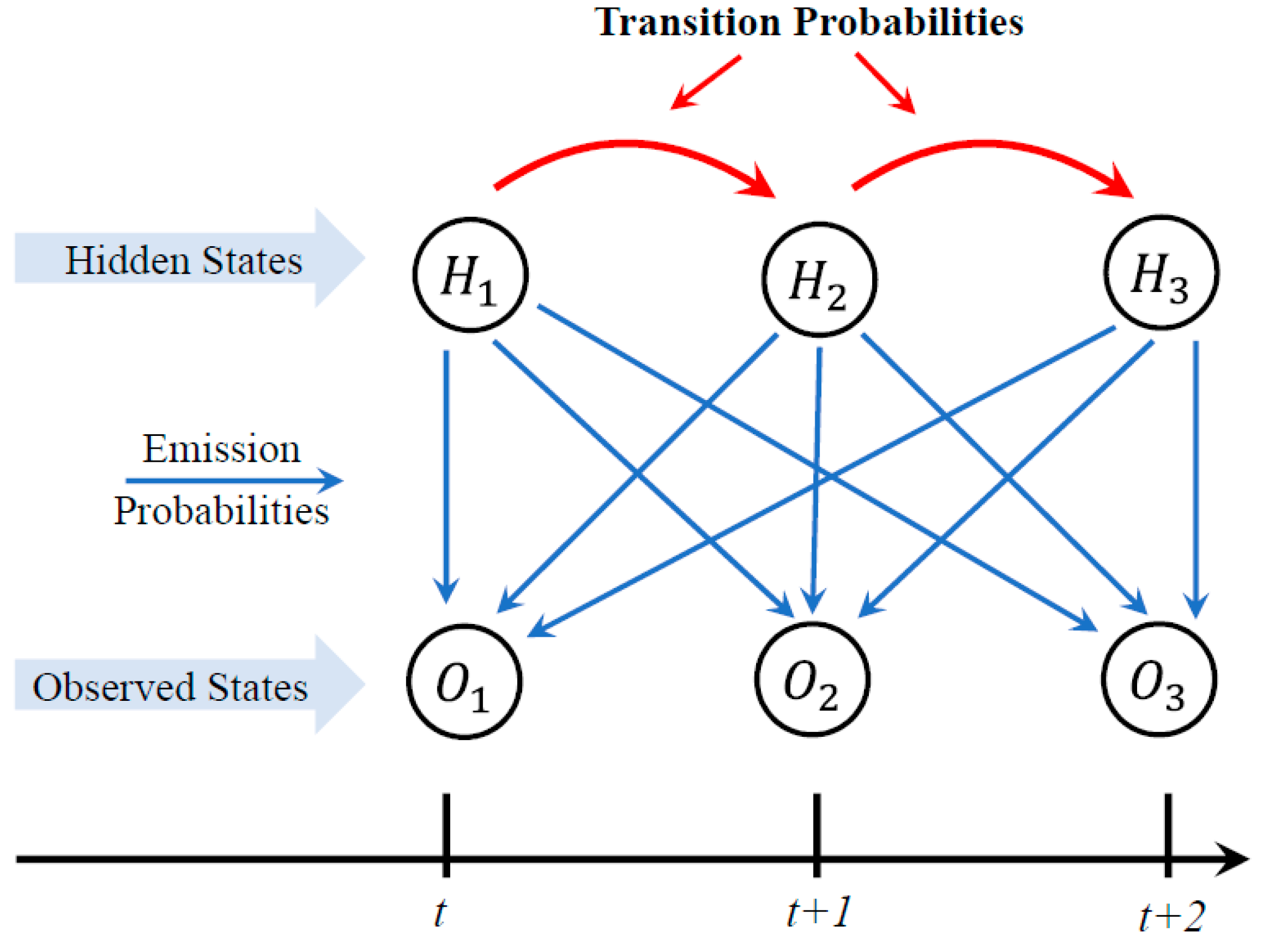
Hidden Markov models (HMMs) assume pavements have two types of condition states: observed states and hidden states. All pavement distresses such as cracking and potholes that can be inspected and measured are observable, whereas pavement condition indices such as PCI and PSR are unobservable or hidden states.
Figure 4 shows the structural and temporal representation of the HMMs. The transition probabilities of the hidden states (i.e.,
) are estimated using the data of the observed states (i.e.,
) and the emission probabilities.
[
52] developed an HMM to predict pavement composite condition index (CCI) when data is incomplete. They assumed that pavement CCI represents roughness and cracking indicators. Pavement roughness data was assumed to be complete while cracking data was assumed to be incomplete. The hidden states were expressed by the CCI, whereas the observed states were expressed by the roughness and cracking indicators. The transition probabilities of the observed states were estimated using the multi-stage hazard methodology of [
56]. The probability distribution of the hidden states was assumed to follow the exponential distribution. The probability distribution, transition probabilities, and exponential rate were estimated using the MLE method and the expectation-maximum algorithm. Data were acquired from Vietnam for Years 2001 and 2004. Pavement sections were grouped into five condition states based on the CCI. The variables traffic volume and pavement thickness were found to be statistically significant in estimating the transition probabilities of pavements in state 2, whereas the pavement thickness was the only statistically significant variable in estimating the transition probabilities of pavements in states 3 or 4. The estimated deterioration rates for pavements in states from 1 to 5 were found to be higher than the typical deterioration rates for typical pavements in Vietnam. To test the capability of the developed model for an incomplete data scenario, only pavement roughness data was used to estimate pavement deterioration rates. The estimated deterioration rates were found to be approximately similar to that when the entire data was used.
[
57] extended their prior work to [
52]to examine the accuracy of predicting pavement condition against the amount of available data. They assumed that the pavement CCI involves the roughness and texture depth of pavement. The transition probabilities of pavement roughness and texture depth were assumed to follow the exponential distribution. [
57] used the data of their 2012 [
52]. Four scenarios of incomplete data were created. The entire roughness data was used in all scenarios, but 100%, 50%, 25% and 10% of the texture depth data was used in scenarios 1, 2, 3 and 4, respectively. The results showed that the total duration taken by newly constructed pavements to move to state 5 is 14 years, which was consistent with pavement deterioration trends in Vietnam. Also, the predicted deterioration rates for pavements in states 1 and 2 were found to be similar across all scenarios. The predicted deterioration rates for pavements in states 3 and 4 for scenarios 2, 3 and 4 were found to be higher than that for scenario 1. These results indicate that the accuracy of pavement condition prediction improves if greater amounts of data are used for the HMM. Additionally, with 50% of the texture depth data the model was capable to predict pavement condition with 3% deviation from the predictions when the entire texture depth data was used. These results indicate that the required amount of data for modeling pavement performance can be reduced if the HMM methodology is used.
[
58] presented an HMM model to estimate pavement cracking rates and potholes for heavy traffic urban roadways in Japan from 2007 to 2011. The cracking rates were modeled using the Markov model developed by [
59]), while the potholes number was modeled using the Poisson process. Markov Chain Monte Carlo simulation and Gipp's sampler algorithm (i.e., Bayesian estimation approach) were used to estimate the models’ parameters. Pavement sections were categorized into five condition states based on the cracking rates; where state 1 represents the lowest cracking rates and state 5 represents the highest cracking rates. The estimated deterioration rates associated with pavements in state 1 were found to be high with a holding time of 7 years. The probability of potholes occurrence is negligible during the first condition state but it goes up during the latter condition states.
Prior research [
52,
57,
58] developed HMMs to predict pavement condition when data is incomplete. Lethanh et al. (2014) did not test the validity of their model with actual data, while [
52,
57] used data for only 2 years which may not be sufficient to capture the historical behavior pavements. Additionally, the estimated transition probabilities were assumed to follow the exponential distribution, which means that pavement deterioration rates were assumed constants. Hence, further research is required to investigate the results of the HMMs when more extensive pavement condition data is employed, and other distribution functions are assumed.
