1. Introduction
Released in 2015, The Residual Network (ResNet) architecture [
1] quickly became a popular model for computer vision tasks due to its simplicity and effective scalability. However soon they were taken over by models that were more memory efficient, had faster inference and better accuracy. As of today, deep learning models like MobileNets [
2], ConvNext [
3], EfficientNet [
4] have outperformed ResNets in a lot of computer vision tasks but these models are generally trained on a larger dataset and transfer learning is performed to finetune it to specific tasks.
Transfer learning might be effective but what about performance while training from scratch. The increased complexity of some models can often lead to higher memory consumption and longer inference times especially as number of parameters increase. These characteristics present substantial challenges for real-world applications where computational resources are limited. And as AI becomes an inevitable part of our daily lives and being increasingly used in embedded systems, these tasks must be performed efficiently with constrained computational capabilities [
5]. Therefore, there is a need for a model that has high accuracy with memory and computational efficiency.
This study aims to optimize and develop a memory-efficient version of the ResNet architecture that maintains competitive performance compared to similar models. The focus is on optimizing the model for deployment in mobile and embedded systems, where resources are constrained. At the same time, proving that an inefficient model like ResNet can be optimized to outperform similar newer models.
The proposed Distilled MixUp Squeeze ResNet architecture incorporates several advanced optimization techniques including commonly used techniques like data augmentation and hyperparameter tuning, and some not so common techniques such as use of Squeeze-Excitation blocks, and knowledge distillation. The work tries to explore the capabilities of optimized ResNets to serve as a new benchmark model for mobile applications pertaining image recognition and classification with limited training and computational resources.
2. Data
The CIFAR-10 dataset [
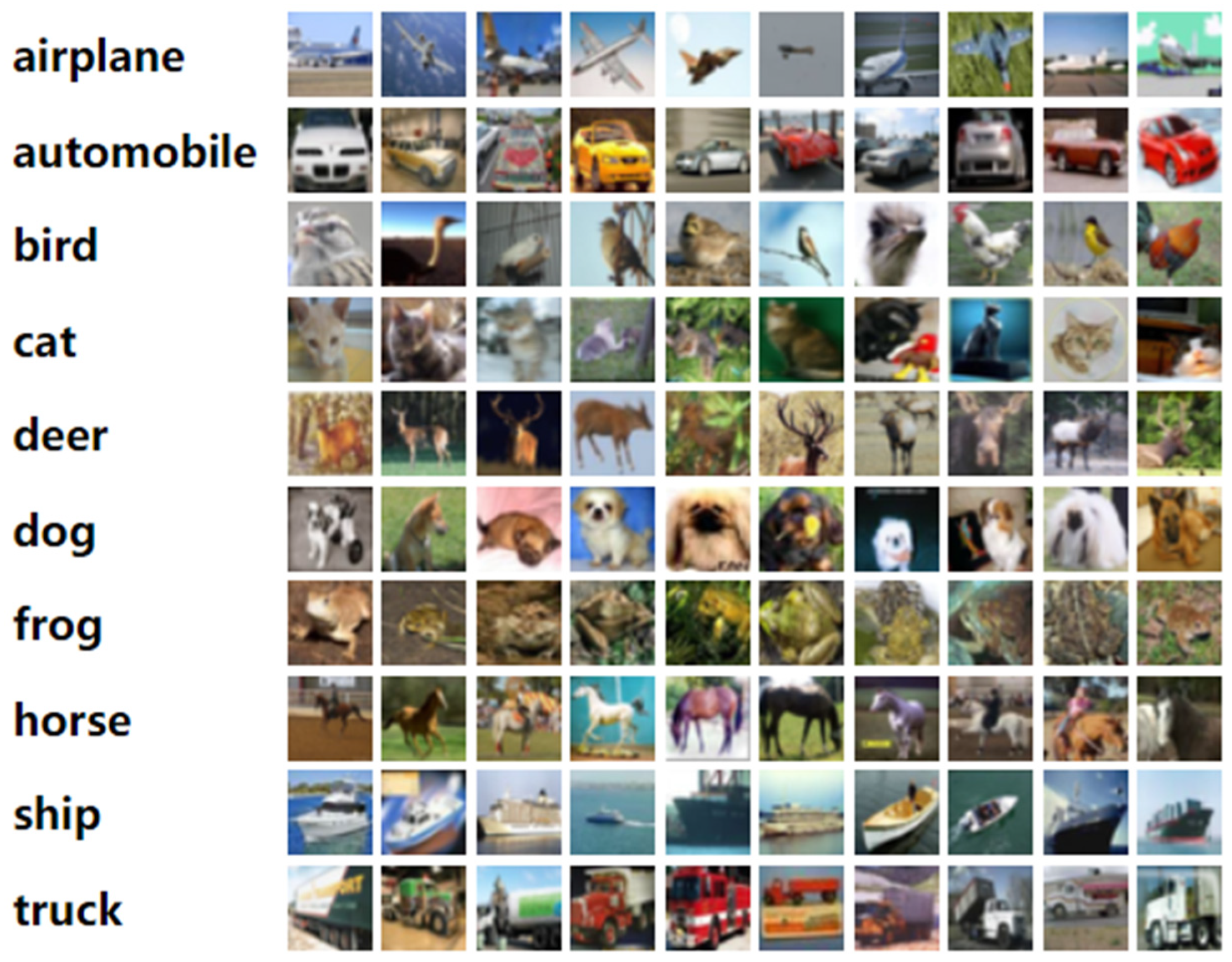
6] is a widely used benchmark dataset in the field of computer vision. It comprises 60,000 32x32 color images distributed across 10 distinct classes, with each class containing 6,000 images. The dataset is divided into 50,000 training images and 10,000 test images. Each image is labeled with one of the following categories: airplane, automobile, bird, cat, deer, dog, frog, horse, ship, or truck.
The CIFAR-10 dataset is popular for several reasons. Firstly, its relatively small image size makes it computationally tractable for training and experimentation, especially when compared to larger datasets like ImageNet. Secondly, the dataset contains a diverse range of object categories, allowing researchers to develop and evaluate models on a variety of visual recognition tasks. Additionally, CIFAR-10 has been extensively studied and used as a benchmark for evaluating the performance of different machine learning and deep learning algorithms.
In the context of this study, the CIFAR-10 dataset serves as the primary dataset for training and validation of the model. The use of CIFAR-10 allows for an evaluation of the model’s performance in image classification tasks within a controlled experimental setup, where the results of use of the same data is widely available and/or easy to reproduce. Moreover, as CIFAR-10 images are relatively low resolution, which is similar to cameras suitable for use in IOT devices, the low resolution enables efficient experimentation and iteration during model development.
3. Methodology
3.1. Proposed Architecture
The model architecture and training is based on existing works on ResNet, incorporating several techniques and experimentally optimized hyperparameters for training a ResNet. It consists of three residual layers configured as follows: the first layer has 4 residual blocks, the second layer has 4 residual blocks, and the third layer has 3 residual blocks. Each residual block employs a convolutional kernel size of 3x3 and a shortcut kernel size of 1x1. The number of channels in each layer is set to 64 for the first layer, 128 for the second layer, and 256 for the third layer. Batch normalization is applied throughout the network to stabilize and accelerate training [
7].
For optimization, Stochastic Gradient Descent (SGD) with a momentum of 0.9 and a weight decay of 0.0005 is used. Data augmentation techniques such as random cropping and horizontal flipping are employed to improve model generalization. To combat overfitting, dropout with a probability of 0.1 is applied. The initial learning rate is set to 0.1, managed by a CosineAnnealing learning rate scheduler. The model is trained with a batch size of 128 for 200 epochs. While extending the training to 400 epochs has shown significant improvements, the training was limited to 200 epochs to adhere to standard practices.
3.2. Building Blocks of Model Architecture
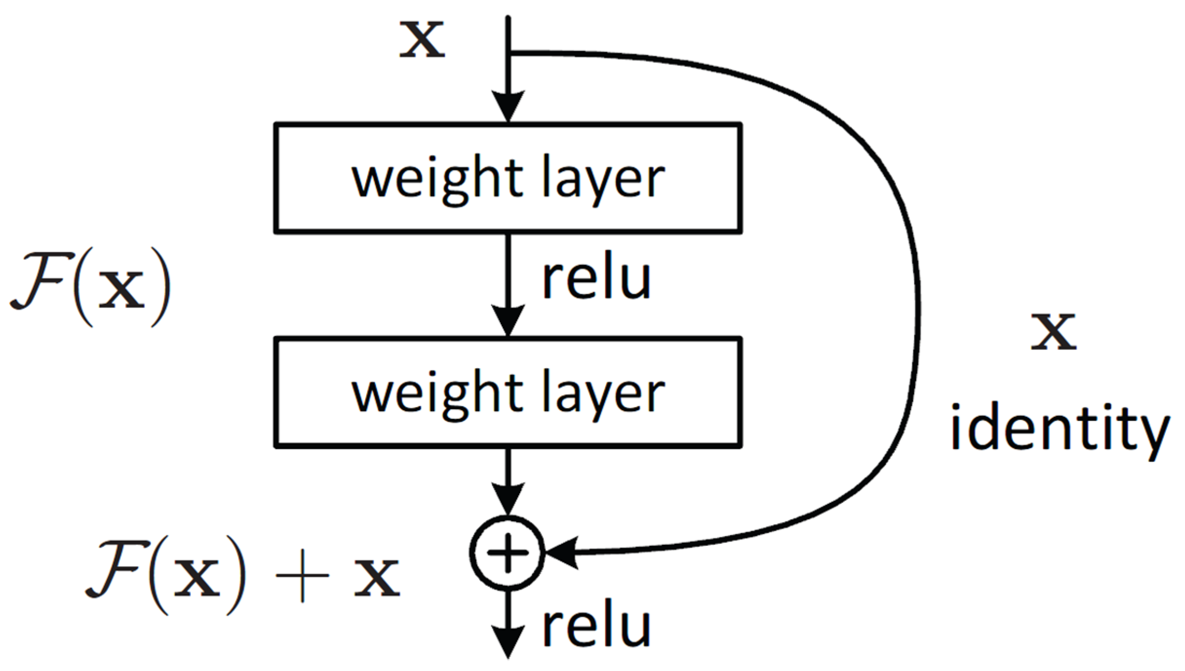
Introduced in 2015, Residual Networks (ResNet) significantly improved the training of deep neural networks by addressing the vanishing gradient problem through the introduction of residual connections. These connections, which act as shortcuts, allow gradients to bypass one or more layers. This mechanism depicted in Image 2, prevents gradient vanishing and facilitates the training of substantially deeper networks.
Image 2.
ResNet Block [
1].
Image 2.
ResNet Block [
1].
ResNet architectures are constructed using two primary types of blocks: basic blocks or bottleneck blocks. The basic block, typically employed in ResNet-18 and ResNet-34, consists of two 3x3 convolutional layers. This structure simplifies network design and reduces computational demands while still benefiting from residual connections that add inputs directly to outputs, thus facilitating training and enhancing performance.
In contrast, the bottleneck block, utilized in deeper ResNets such as ResNet-50, ResNet-101, and ResNet-152, comprises three layers (1x1, 3x3, and 1x1 convolutions). The 1x1 layers are responsible for dimension reduction and projection, effectively managing the network’s complexity and computational load. This configuration enables the significant extension of network depth without a substantial increase in resource requirements. The proposed model uses Basic Block because of its smaller size and Squeeze Excitation blocks because of their ability to generate channel wise attention to create the Residual neural network.
3.2.1. Basic Convolutional Block
The Basic Convolutional Block, also referred to as the BasicBlock, forms the fundamental component of the ResNet architecture. It comprises two convolutional layers, each succeeded by batch normalization to stabilize and accelerate training. The first convolutional layer employs a 3x3 kernel with a specified stride, while the second convolutional layer maintains the input size. An integral shortcut connection bypasses these layers, facilitating gradient flow during training.
3.2.2. Squeeze-and-Excitation (SE) Block
The Squeeze-and-Excitation (SE) Block [
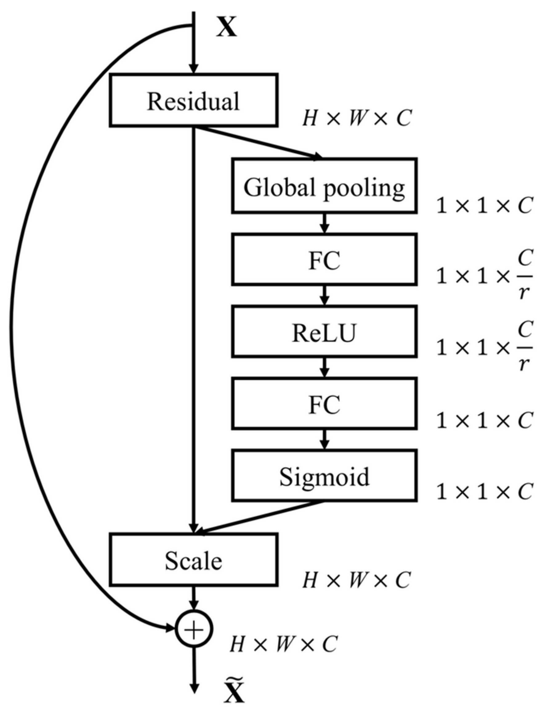
8] improves feature recalibration by adaptively weighting channel-wise feature responses within the network. This block integrates two convolutional layers with a global average pooling operation to capture channel-wise statistics. The first convolutional layer reduces the number of channels, thereby improving computational efficiency, while the subsequent activation function introduces non-linearity. The final convolutional layer restores the original channel dimensionality, and a sigmoid activation function scales the features, emphasizing the most informative channels.
Image 3.
SE-ResNet Module [
8].
Image 3.
SE-ResNet Module [
8].
3.2.3. Residual Layers
The Residual Layers encapsulate multiple instances of the Convolutional Block, forming the core structure of the ResNet architecture. Each Residual Layer comprises a sequence of BasicBlocks, with the number of blocks determined by the specified architecture configuration. The stride parameter controls the downsampling of feature maps within each layer, facilitating the extraction of features at multiple scales. The inclusion of skip connections mitigates the vanishing gradient problem, enabling effective gradient flow during training. This hierarchical arrangement of Residual Layers enables the network to learn increasingly abstract representations of the input data, leading to improved classification performance.
3.3. Loss Function
3.3.1. Mixup Augmentation Loss
Mix-up augmentation technique [
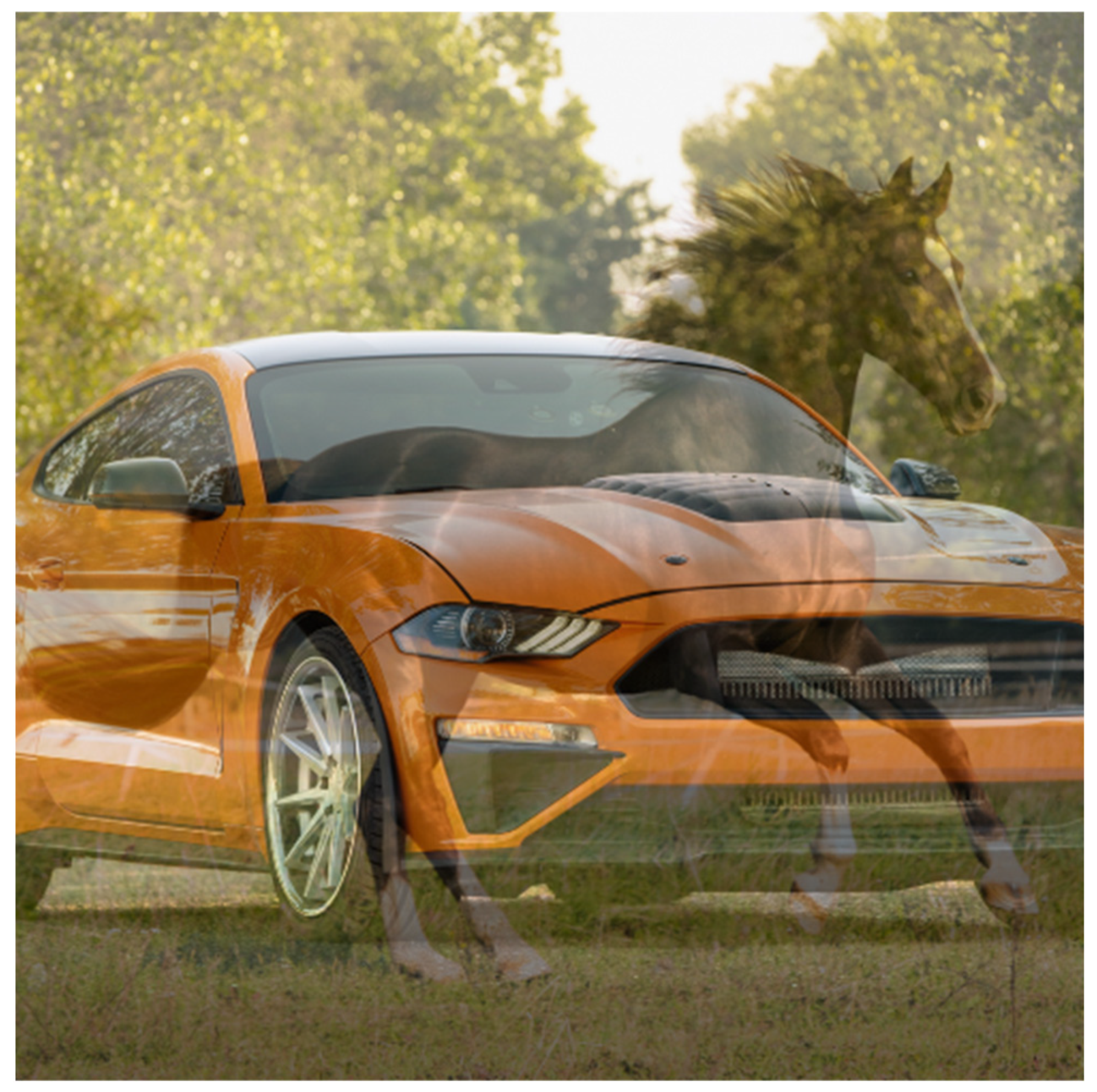
9] is designed to improve the generalization of image classification models by training on linear combinations of image pairs and their labels. The images are mixed, and each image is assigned the corresponding set of mixed labels, as seen in Image 4. Hence, promoting the model to learn more robust features that are not tied to specific training examples.
Image 4.
Image showcasing mixup augmentation between images of a horse and car; labels (horse, car).
Image 4.
Image showcasing mixup augmentation between images of a horse and car; labels (horse, car).
The primary benefits of using Mix-up include reducing the risk of overfitting by smoothing the label space and enhancing model robustness against noisy data. It also stabilizes the training process, leading to more reliable convergence.
A mixUp loss function which is a loss function consisting of the sum of losses of mixed images on both of its true labels. Described in equation (i), is used to train the model containing datasets with mixup augmentation.
Loss is any loss function chosen for training. Lambda is the weight of each label in the image.
is predicted label, and label A and label B are true labels.
3.3.2. Knowledge Distillation Loss
Knowledge distillation [
10] is a technique used for transferring knowledge from a large, complex teacher model to a smaller, more efficient one known as a student model. It involves training the student model to mimic the soft output (class probabilities) of the teacher model rather than the hard targets (actual class labels). The soft probabilities contain richer information about the input space as they reflect the confidence of the teacher model across all classes.
There are several ways to perform knowledge distillation, a loss based distillation was used for simplicity and ease of addition to the model. Image 5 depicts the working of a knowledge distillation architecture based on this technique.
The knowledge distillation loss combines the Kullback-Leibler divergence and any relevant loss function, for consideration, the cross-entropy loss, to train a student network effectively using a teacher network’s predictions. The first term measures the divergence between the log-softmax of the student network’s outputs
Zs and the softmax of the teacher network’s outputs
Zt, both scaled by a temperature parameter
T. The second term measures the cross-entropy between the student network’s outputs and the soft targets provided by the teacher network. This term is weighted by 1−α balancing the influence of the distillation loss and the traditional loss. This approach ensures that the student network learns from both the softened outputs of the teacher network and the ground truth labels, improving generalization and performance. The equation for this knowledge distillation loss is given below in equation (ii):
is a weight for each function, Kld represents a function of KL divergence, represents softmax function, Zs and Zt represent logits of Student and Teacher models respectively, Loss is any loss function that can be used relevant to the task at hand.
3.3.3. CrossEntropy Loss
At the core of the loss functions used in neural networks is the Cross-Entropy Loss. This loss function measures the performance of a classification model whose output is a probability value between 0 and 1. The Cross-Entropy Loss increases as the predicted probability diverges from the actual label. Mathematically, it is defined as Equation (iii),
In this formula, denotes the true labels, and signifies the predicted probabilities. This loss function effectively penalizes incorrect classifications more heavily, hence training models to make better predictions.
3.3.5. Model Training Loss
The training loss used for the model is a knowledge distillation loss combined with Mixup loss. The Cross-entropy loss is used as the model loss to build upon our derived loss functions.
Using equations (i) and (ii), the derived loss can be written as,
Hence, the equation for the training loss is given in Equation 4 as,
Note: CrossEntropy Loss is written as CELoss for convenient representation.
Hence, the proposed training loss function effectively integrates knowledge distillation and Mixup loss to enhance model performance. The knowledge distillation loss allows for efficient transfer of knowledge from a teacher model to a student model, while the Mixup loss improves generalization by interpolating between data samples. The derived loss function, as presented in Equation (iv), balances these components to optimize the training process, combining their strengths to improve accuracy and robustness. This approach enhances the model’s learning capacity and ensures it is well-prepared to handle diverse and challenging data scenarios, providing a solid framework for advanced model training.
3.4. Training
The primary ResNet architecture described in
Section 3.1, using a cross entropy loss function described in
Section 3.3.3 was trained for 200 epochs to train the first model containing only ResNet + Squeeze Excitation based architecture.
Adding mixup augmentation to train the same architecture, required using a mixUp loss, based on use of cross entropy loss, as the
Loss function described in equation (i) in
Section 3.3.1. Obtaining the ResNet + Squeeze Excitation + MixUp, which was again trained for 200 epochs.
For knowledge distillation, a ResNet50 architecture containing BottleNeck blocks, SE blocks and mixUp augmentations, trained for 200 epochs was used as the teacher, its weights were distilled onto the exact same setup as model using ResNet + Squeeze Excitation + MixUp using loss function described in
Section 3.3.5 to train the model.
4. Results and Discussion
The proposed Distilled MixUp Squeeze Residual Network (DMSResNet) architecture, comprising 4,367,742 parameters, was rigorously evaluated on the CIFAR-10 dataset. A series of configurations and optimization techniques were examined to determine their influence on the model’s performance.
Table 1 presents a comparative analysis of various models, highlighting their training accuracy and validation accuracy.
The baseline ResNet model achieved a training accuracy of 100% due to overfitting and a validation accuracy of 81.79%. The integration of Squeeze-and-Excitation (SE) blocks into the ResNet model led to significant improvements, yielding a training accuracy of 99.99% and a validation accuracy of 95.51%. This enhancement demonstrates the effectiveness of SE blocks in improving model performance by re-calibrating channel-wise feature responses.
Further improvements were observed with the incorporation of MixUp data augmentation. The model, enhanced with both SE blocks and MixUp, achieved a training accuracy of 52.43% and a validation accuracy of 96.46%. The lower training accuracy indicates that MixUp augmentation successfully mitigates overfitting, while the higher validation accuracy highlights its ability to enhance generalization.
The application of knowledge distillation where the student model learns from a larger teacher model, resulted in comparable performance to the SE and MixUp-augmented model. The KD-enabled DMSResNet achieved a training accuracy of 52.90% and a validation accuracy of 96.56%. This outcome demonstrates the combined effectiveness of SE blocks, MixUp augmentation, and KD techniques in improving model performance within stringent parameter constraints.
These results indicate that the proposed DMSResNet architecture achieves high accuracy rates on the CIFAR-10 dataset while adhering to parameter constraints. The integration of SE blocks, MixUp augmentation, and Knowledge Distillation techniques collectively contribute to the model’s enhanced performance. Future comparisons with other models trained from scratch without transfer learning or additional data would provide further insights into the significance of these results.
5. Conclusions
The DMSResNet model has demonstrated significant improvements in accuracy on the CIFAR-10 dataset while maintaining a compact architecture. These enhancements showcase the potential of combining advanced techniques to optimize deep learning models for performance and efficiency, particularly in resource-constrained environments such as mobile and embedded systems.
Future work can expand upon these findings in several ways. First, exploring the application of these optimization techniques to other deep learning architectures can validate their generalizability and effectiveness across different network designs. Additionally, investigating the impact of these techniques on larger and more diverse datasets will provide insights into their scalability and robustness.
Another interesting idea would be to try distilling a very large model which performs very well on the dataset, using VIT (Vision Transformers) would be an interesting experiment for distillation.
Moreover, the exploration of hardware-specific optimizations, such as leveraging quantization and pruning techniques tailored to the unique requirements of mobile devices, could further reduce the model’s footprint and improve inference speed without compromising accuracy.
By building on the foundation set up by the work, future research can continue making AI capabilities more accessible and practical across IOT/ light hardware devices for computer vision applications.
References
- Kaiming He, Xiangyu Zhang, Shaoqing Ren, and Jian Sun. Deep residual learning for image recognition, 2015.
- Andrew, G. Howard, Menglong Zhu, Bo Chen, Dmitry Kalenichenko, Weijun Wang, Tobias Weyand, Marco Andreetto, and Hartwig Adam. Mobilenets: Efficient convolutional neural networks for mobile vision applications, 2017. [CrossRef]
- Zhuang Liu, Hanzi Mao, Chao-Yuan Wu, Christoph Feichtenhofer, Trevor Darrell, Saining Xie; A ConvNet for the 2020s, Proceedings of the IEEE/CVF Conference on Computer Vision and Pattern Recognition (CVPR), 2022, pp. 11976-11986.
- Tan, Mingxing, and Quoc Le. “Efficientnet: Rethinking model scaling for convolutional neural networks.” International conference on machine learning. PMLR, 2019.
- Gaurav Menghani. 2023. Efficient Deep Learning: A Survey on Making Deep Learning Models Smaller, Faster, and Better. ACM Comput. Surv. 55, 12, Article 259 (December 2023), 37 pages. [CrossRef]
- Alex Krizhevsky. Learning multiple layers of features from tiny images. pages 32–33, 2009.
- Aditya Thakur, Harish Chauhan, and Nikunj Gupta. Efficient resnets: Residual network design. arXiv preprint. arXiv:2306.12100, 2023.
- Jie Hu, Li Shen, Gang Sun; Squeeze-and-Excitation Networks, Proceedings of the IEEE Conference on Computer Vision and Pattern Recognition (CVPR), 2018, pp. 7132-7141.
- Hongyi Zhang, Moustapha Cisse, Yann N Dauphin, and David Lopez-Paz. mixup: Beyond empirical risk minimization. arXiv preprint. arXiv:1710.09412, 2017.
- Geoffrey Hinton, Oriol Vinyals, and Jeff Dean. Distilling the knowledge in a neural network, 2015.
- Assiri, Yahia. “Stochastic optimization of plain convolutional neural networks with simple methods. arXiv:2001.08856 (2020).
- Hassani, A., Walton, S., Shah, N., Abuduweili, A., Li, J., & Shi, H. (2021). Escaping the big data paradigm with compact transformers. arXiv preprint. arXiv:2104.05704.
- Yang, C., An, Z., Zhu, H., Hu, X., Zhang, K., Xu, K., … & Xu, Y. (2020, April). Gated convolutional networks with hybrid connectivity for image classification. In Proceedings of the AAAI conference on artificial intelligence (Vol. 34, No. 07, pp. 12581-12588).
Table 1.
Model Performance Comparison.
Table 1.
Model Performance Comparison.
| Model |
Accuracy |
Parameters |
Epochs |
| Stochastic Optimization of Plain CNNs [11] |
94.29% |
4.3M |
2500 |
| CCT-7/3x1 [12] |
96.53% |
3.76M |
300 |
| HCGNet-A2 [13] |
97.71% |
3.1M |
1260 |
| ResNet + Squeeze Excitation |
95.51% |
4.3M |
200 |
| ResNet + Squeeze Excitation + MixUp |
96.46% |
4.3M |
200 |
| KDistillation DMSResNet |
96.56% |
4.3M |
200 |
|
Disclaimer/Publisher’s Note: The statements, opinions and data contained in all publications are solely those of the individual author(s) and contributor(s) and not of MDPI and/or the editor(s). MDPI and/or the editor(s) disclaim responsibility for any injury to people or property resulting from any ideas, methods, instructions or products referred to in the content. |
© 2024 by the authors. Licensee MDPI, Basel, Switzerland. This article is an open access article distributed under the terms and conditions of the Creative Commons Attribution (CC BY) license (https://creativecommons.org/licenses/by/4.0/).


