1. Introduction
Symmetry and balance are widely used in various fields, such as modeling design, architectural design, artistic creation, etc. Symmetry always implies balance, but balance does not necessarily imply symmetry. The factors that affect balance are diverse and complex. This study hopes to explore the method of quantifying balance and its role in aesthetic evaluation through an interdisciplinary research method.
In 2005, the concept of computational aesthetics was first put forward at the International Conference on Computational Aesthetics in Graphics, Visualization and Imaging of the Eurographics Association. Computational aesthetics is the study of computational methods that can make appropriate aesthetic decisions in a way similar to that of humans [
1]. The primary research methods in computational aesthetics encompass convention approaches with handcrafted features, as well as aesthetic judgment tasks employing deep learning techniques [
2]. In this study, we take the balanced composition in art history as the research object, systematically investigating the quantification of balanced composition, its relationship with aesthetics. The term "composition" originates from the Latin word "composito," which can be translated as "arrangement" or "organization"[
3]. The principle of unity guides this process by ensuring the elements produce a harmonious aesthetic, and balance is an important means to achieve unity [
4]. Arnheim argued that the sense of balance is a psychological need: "When people looked at pictures, they naturally sought a state of stability and balance"[
5]. By adhering to specific methods, creators can achieve well-balanced in paintings, ensuring that the elements in the work reach a harmonious and stable visual state, resulting in a composition that is beautiful [
3,
6].
Although beauty has no absolute criterion, it possesses universality. Chatterjee et al. [
7] suggested that art possesses a dual nature: it is both highly varied and culturally diverse, yet also universal and common to all humans. Zeki divided sensory experiences, including those from aesthetic sources, into two main categories: the aesthetic experience of biological beauty, and the experience of artifactual beauty [
8,
9]. Research indicates that balance affects eye movements and can function as a primitive visual operating system, the ability to discern balanced compositions was independent of an individual's level of art education, both individuals with and without an artistic background could quickly determine whether a picture was balanced or not, balance as fundamental principles in the organization and biology of organic forms, humans share an inherent sense of composition, derived from our innate ability to recognize organic form [
10,
11,
12,
13,
14]. However, the manifestation of balanced composition varies across different types of pictures, not all balanced compositions will necessarily appeal to people [
15,
16].
It is generally believed that a pictorial configuration is considered balanced when its elements and their qualities are poised or organized around a balancing center, giving the appearance of being anchored and stable [
17]. Balance can be attainedable in various ways, primarily encompassing symmetrical and asymmetrical distributions. Symmetrical balance pertains to the symmetrical allocation of elements on either side of the central axis within the picture, engendering mirror symmetry. Symmetry is a significant and conspicuous characteristic of the visual realm, and it is regarded as the foundation of image segmentation and perceptual organization, while also exerting a role in more advanced processes [
18]. Enquist et al. [
19] that the ubiquity of symmetry in nature and decorative art could be attributed to the sensory bias towards symmetry in humans and other organisms, which has been independently exploited by natural selection acting on biological signals and by human artistic innovation. Certain studies have revealed that even infants are already capable of efficiently processing vertically symmetrical patterns, suggesting that the recognition of vertical symmetry may be innate or acquired at a very early stage [
20]. Guy et al. [
21] propose that stimulus symmetry might induce selective attention to the global properties of a visual stimulus, thereby facilitating higher-level cognitive processing in infancy. Other studies have discovered that for adults, symmetry demonstrates a strong positive correlation with aesthetic judgment [
22,
23,
24]. Certainly, the process of aesthetics is complex, and factors such as educational background, cultural differences, and professional knowledge level can all have an impact on aesthetics. Leder et al.'s [
25] research discovered that in the task of rating beauty, compared with art historians and non-experts, art experts regarded asymmetrical and simple stimuli as the most beautiful, which demonstrated the influence of education and training on aesthetic appreciation. Asymmetrical balance refers to the visual asymmetry of elements in a picture, but through the ingenious arrangement of factors such as color, shape, and size, the whole still appears harmonious and stable. Asymmetrical balance is typically more dynamic, which can arouse a deeper level of interest and discussion from the audience. Studies have discovered that when adults arrange picture elements on circular and rectangular backgrounds, they will use the center of the picture as the "anchor" to evenly distribute the structure or physical weight of the elements around the main axis of the design throughout the entire structure [
17,
26].
Many studies on balanced composition focus on this "anchor". Wilson and Chatterjee proposed a method for quantifying balanced composition called the Assessment of Preference for Balance (APB). This method involves centering on the midpoint of the picture and using the main axes—the vertical, horizontal, and two diagonal axes. The black pixel ratios of the equal-area regions on both sides of, and inside and outside, the corresponding axes are quantified. The overall balance value is then determined by averaging these eight balance ratios [
27]. Some scholars have also put forward that the degree of deviation between the center of gravity and the center of the picture can be used as a quantitative indicator of balance [
28]. Research has shown that using the deviation of the center of mass as a quantitative indicator of the balanced composition of multi-object and dynamic-pattern patterns is positively correlated with the degree of favorability [
29]. Alternatively, in a polar coordinate system, an angle variable can be added based on the Euclidean distance to quantify the balance [
30]. Some studies use the more robust Manhattan distance instead of the Euclidean distance [
31].
Through rational composition, the blank negative space can also be a part of the balanced composition. The negative space can be deliberately designed to represent significant content in the scene [
32,
33]. By leaving blank areas around the main subject, the viewer's attention can be naturally guided to focus on the main subject, thereby enhancing the visual impact. Appropriately distributing negative space in the picture can balance the visual weight, achieving an overall harmonious effect. For the quantification of blank space, some researchers directly obtain it by using the ratio of the pixels of the blank area to the total pixels of the picture [
34]. However, some scattered color blocks do not affect the viewer's overall impression of the painting. Therefore, in some studies, when calculating the blank space, only the larger white areas in the painting are considered as the blank area by partitioning the blank area [
31].
To unveil the cognitive processes involved in the creation and appreciation of artworks, using neurological terminology to explain art has become a trend, and the study of aesthetics is gradually shifting from basic visual functions to a comprehensive neurobiological theory of art. Semir Zeki defined neuroaesthetics as the study of the neural basis for the contemplation and creation of a work of art, which reflects the intersection of neuroscience, psychology, and aesthetics [
35,
36]. Chatterjee et al. characterized neuroaesthetics as the cognitive neuroscience of aesthetic experience, suggesting that aesthetic experiences likely emerge from the interaction between emotion-valuation, sensory-motor, and meaning-knowledge neural systems [
37,
38]. Balance composition is closely related to aesthetics, in their explorations artists are unconsciously exploring the organization of the visual brain though with techniques unique to them [
39]. The ERP method enables researchers to identify the mental processing modes involved in cognitive and aesthetic processing. Many studies have used this method to investigate the connection between visual features and aesthetics, analyzing the cognitive processing of various features and their association with aesthetic judgments [
22,
40,
41,
42]. Utilizing EEG experiments, participants undertake different feature judgment tasks and aesthetic judgment tasks on the same stimuli. Through ERP data, the relationship between these tasks can be analyzed to examine the cognitive processes involved in feature evaluation and aesthetic evaluation.
Neuroaesthetics is devoted to investigating the cognitive mechanism of aesthetics and the relationship between hand-crafted features and aesthetics, while computational aesthetics possesses distinct advantages in quantifying hand-crafted features and establishing machine learning models. Certain scholars have put forward the notion that by integrating the methods of neuroaesthetics and computational aesthetics through an interdisciplinary approach, it becomes feasible to more effectively predict human aesthetic preferences [
43,
44]. This study presents a systematic idea for studying balanced composition from the aesthetic object to the aesthetic subject, combined with the style of the experimental materials in this study, appropriate parameters can be selected to more accurately quantify these hand-crafted features. Subsequently, employing EEG experiments, the EEG data of the subjects during the processes of aesthetic judgment and balance judgment are obtained, and the relationship between the two tasks is examined through the analysis of ERP data. Finally, the research results are verified by constructing a machine learning model using the method of computational aesthetics, and relevant discussions on the interdisciplinary integration of aesthetic research are carried out.
2. Materials and Methods
2.1. Materials
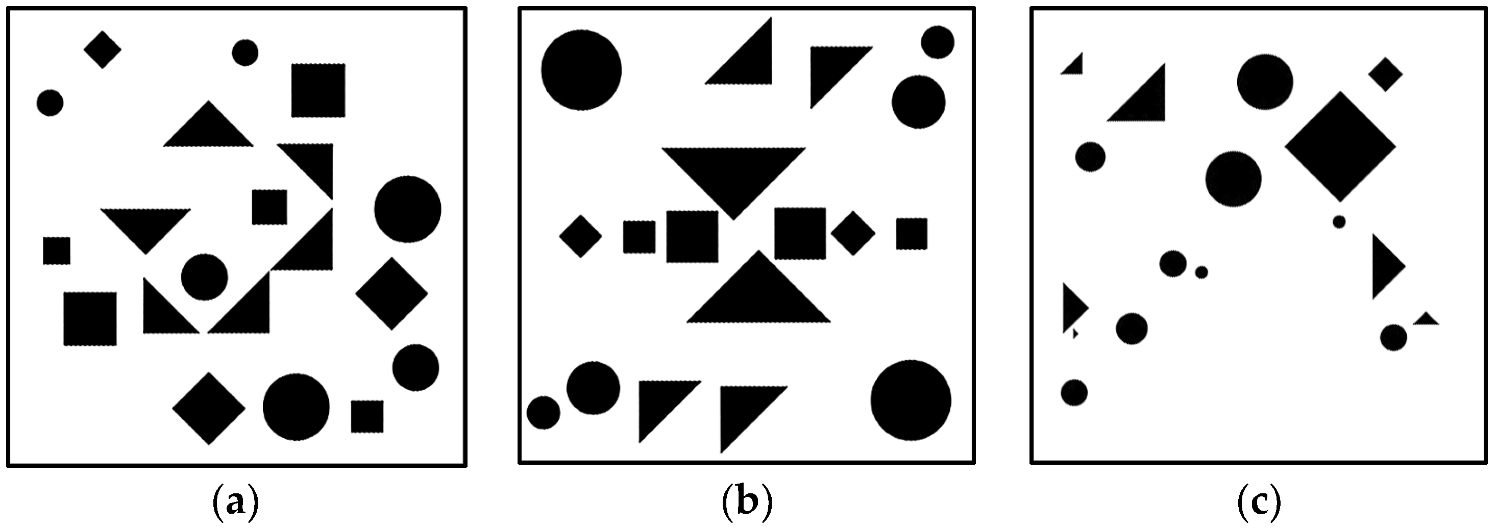
All stimulus materials were generated using Processing5.0 software by configuring various parameters. All stimulus materials have a resolution of 300dpi, and on a white background with a dimension of 500×500 pixels, several black squares, isosceles right triangles, and circles of different sizes are randomly and non-overlappingly distributed, as depicted in
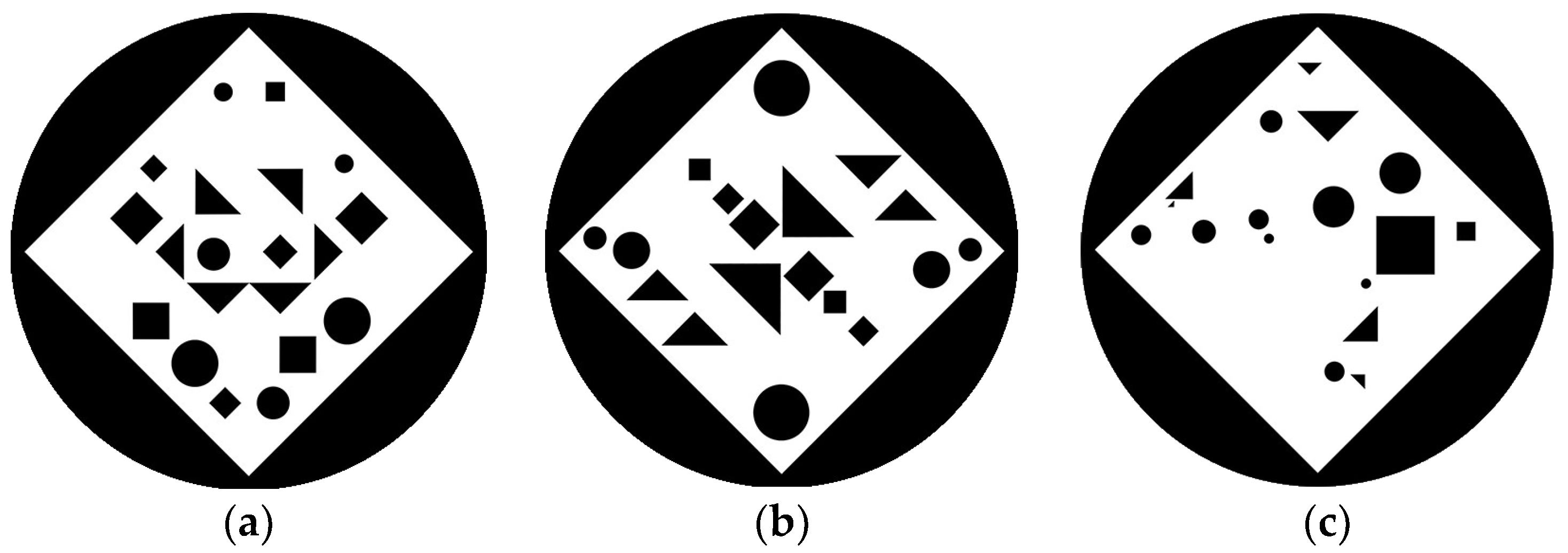
Figure 1. Next, the image was rotated 45° clockwise, and a black circular background was added as the subsequent experimental material, as shown in
Figure 2. Subsequently, the balance parameters of the experimental materials were quantified. In this study, three parameters were utilized to quantify the balance: symmetry, center of gravity, and negative space.
2.2. Parameters of Balance
2.2.1. Symmetry
Symmetry encompasses left-right symmetry and central symmetry. Left-right symmetry pertains to the mirror symmetry of the content on the left and right sides of the image, while central symmetry refers to symmetry around the center of symmetry.
In this study, by counting the number of pixels with different positions on the left and right sides of the image with the central axis as the symmetry axis, the same method was also used to quantify the central symmetry value. As long as one of the two symmetries was fulfilled, the image could be regarded as symmetrical. Hence, through the quantification results, the closer symmetry type of the image could be determined, and this outcome was utilized as the symmetry value of the image.
2.2.2. Center of Gravity
The overall distribution of the picture is quantified by the degree of deviation of the picture's center of gravity. Firstly, the coordinates of the center of gravity
and the center of the image
are obtained, and subsequently, the Manhattan distance between the two is computed:
Here, is the pixel value (0 or 1) of the image at position , W is the width of the image, and H is the height of the image.
2.2.3. Negative Space
The quantification of negative space necessitates the division and feature extraction of the picture space, Quadtree is a data structure, and its fundamental concept is to recursively divide the two-dimensional space into a tree structure of varying levels [
45].
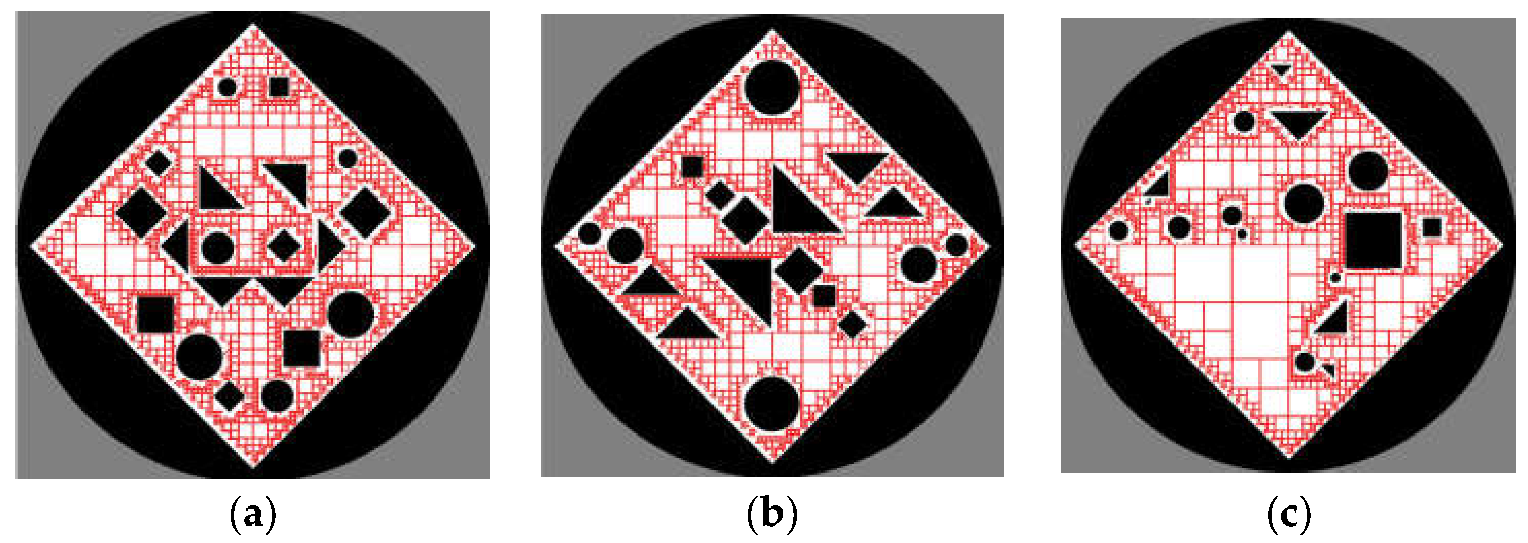
In this study, the image was initially divided into four quadrants, and subsequently, each quadrant was inspected to determine if it was blank. If the quadrant was blank, the area of the quadrant was recorded; then, the non-blank quadrants were recursively subdivided until the termination condition was satisfied, as depicted in
Figure 3.
The area of all white regions is recorded as , which serves as an indicator of the overall contrast of the picture. During the recursive process, a termination condition is set, and the last two results are removed. The prominent large white area is considered the main blank area and recorded as . Despite similar blank areas, the distribution of the blank area might vary. Some blank spaces are extensive and broad, while others are small and fragmented. The largest white rectangle obtained in the recursive process is utilized as a characteristic index to assess different blank spaces and is recorded as .
2.3. Stimulus
From the materials generated by the software, through the experimenters' screening, some materials with similar facial expressions were excluded, and ultimately 279 materials were retained as experimental materials. Visual Studio 2019 software and the open-source computer vision and image processing library Open Source Computer Vision Library (OpenCV) were used to extract and quantify the features of the experimental materials. Based on the feature data, IBM SPSS Statistics 26 software was used for second-order clustering processing, and the experimental materials were divided into two categories, as shown in
Table 1. Type I of materials (N=137) are more symmetrical, with a smaller negative space area and a center of gravity closer to the center of the picture; Type II materials (N=142) are more asymmetrical, with a larger negative space area and a center of gravity farther from the center of the picture. Type I materials are more in line with the balanced composition in the general sense, so they are defined as "balance" in this study. Conversely, Type II materials are classified as "imbalance".
2.4. Electroencephalography (EEG) and Event-Related Potentials (ERP)
In 1924, Hans Berger measured the electrical activity of the human brain by positioning electrodes on the scalp and amplifying the signals, thereby discovering electroencephalography (EEG) [
46]. In 1964, the research report of Gray Walter and his colleagues presented the first ERP component - contingent negative variation [
47]. The electroencephalogram reflects thousands of simultaneous brain processes, implying that the brain's response to a single stimulus or point of interest is usually not visible in the EEG recording of a single trial. However, by performing multiple trials and superimposing and averaging the results, the random brain activity can be averaged out, and the relevant waveforms, namely ERP, can be retained. Through the provision of continuous measurements of the processing between stimuli and responses, the impact of specific experimental conditions on each stage can be determined.
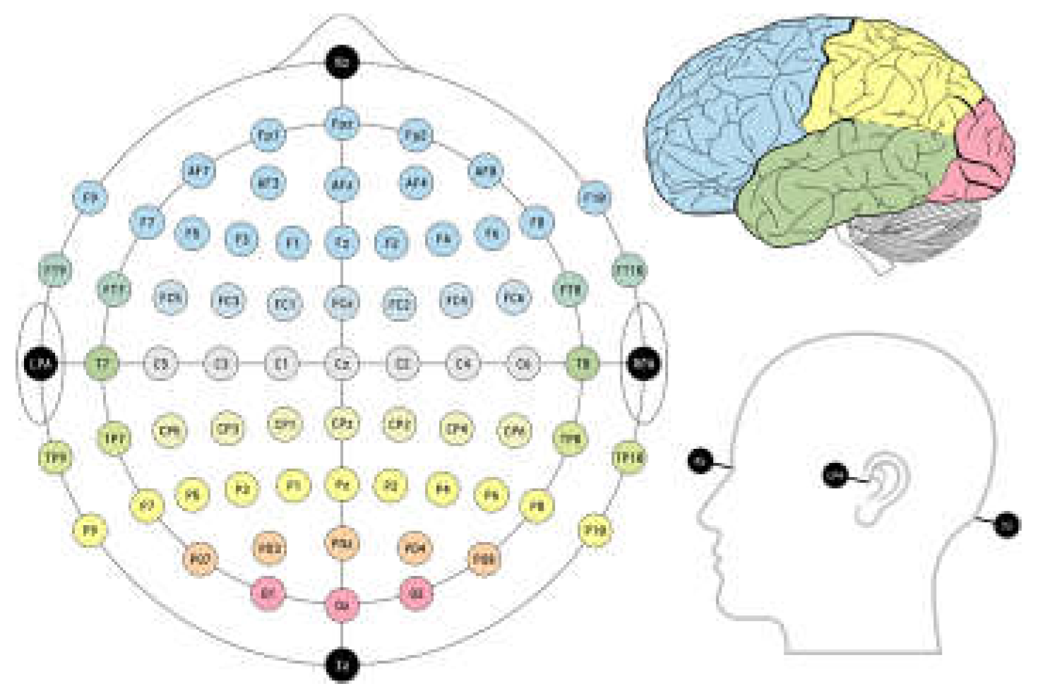
Figure 4.
10-20 System and Brain Region Division (Image sourced from Wikipedia).
Figure 4.
10-20 System and Brain Region Division (Image sourced from Wikipedia).
Different regions of the brain have distinct functions. The electrode distribution utilized in EEG experiments is the international 10-20 system, and each electrode placement site is identified by a letter denoting the brain lobe or region it is monitoring: the prefrontal lobe (Fp), frontal lobe (F) are situated in the anterior portion of the brain, predominantly responsible for advanced cognitive functions, emotional regulation, decision-making, and behavioral control. The parietal lobe (P) is located at the top of the brain and is mainly involved in perception processing, spatial cognition, attention, and working memory. The central region (C) is positioned in the central part of the brain, encompassing the motor cortex and sensory cortex, and is associated with processes such as motor execution, sensory processing, and motor control. The occipital lobe (O) is located at the back of the brain and is primarily responsible for visual processing and visual cognition, and is related to processes such as visual attention, visual recognition, and visual memory. "Z" (zero) refers to the electrodes placed on the midline sagittal plane of the skull (Fpz, Fz, Cz, Oz), while even electrodes (2, 4, 6, 8) indicate the electrodes placed on the right side of the head, and odd electrodes (1, 3, 5, 7) refer to the electrodes placed on the left side of the head; M (or A) denotes the prominent bony protrusion typically found behind the outer ear, and M1 and M2 are used as contralateral references for all EEG electrodes.
2.5. Participant
In this experiment, 18 graduate students were recruited from the College of Mechanical Engineering and Automation, Huaqiao University, including 14 males and 4 females, aged between 22 and 30 years old. All the participants were right-handed and had not received systematic art education, and their vision or corrected vision was normal. Before the experiment, sufficient communication was conducted, and the participants signed the informed consent form. As compensation after the experiment, each participant received 50 yuan. All the procedures and protocols of this experiment were approved by the School of Medicine, Huaqiao University.
2.6. Procedure
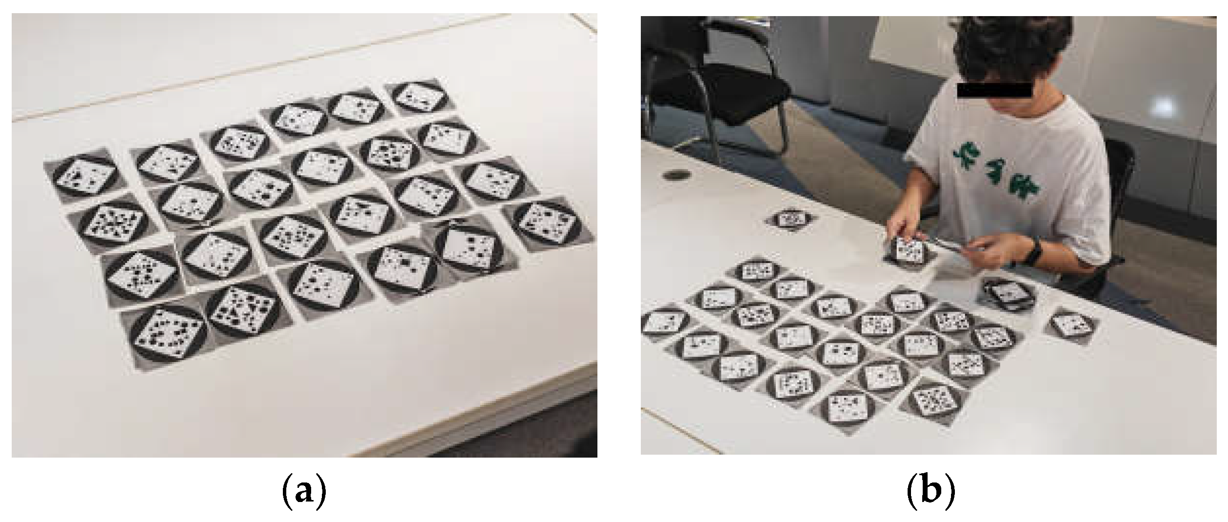
The experimental materials were printed on 85mm×85mm cards and randomly presented to the participants. The participants were required to quickly browse and determine the style of the experimental materials, and then, based on their personal aesthetic standards, categorize the materials into three groups: at least 80 beautiful ones, at least 80 not beautiful ones, and the remaining ones with no feeling or indistinguishable. After completing the categorization, the experimenter would randomly select 5-10 materials for the participants to judge to ensure the accuracy of the classification. If there was a high error rate, the participants would be required to reclassify. There was a maximum of 3 days between the pre-experiment and the main experiment (mostly the next day), to ensure that in the main experiment, the participants could correctly distinguish between beautiful and not beautiful experimental materials.
Figure 5.
Pre-experiment:(a) Randomly Present the Printed Experimental Materials on the Desktop; (b)Participant Classifying Experimental Materials Based on Aesthetic Standards in the Pre-Experiment.
Figure 5.
Pre-experiment:(a) Randomly Present the Printed Experimental Materials on the Desktop; (b)Participant Classifying Experimental Materials Based on Aesthetic Standards in the Pre-Experiment.
In the main experiment, aesthetic judgment task and balance judgment task were completely crossed, and all stimulus materials were presented in a random order. Before the main experiment, the experimenter will give the participants "aesthetic education," using the characteristics of type I materials as the balance index, and convey the form of balanced composition to the participants through verbal expression. During the experiment, the participants are required to concentrate and place the middle finger or index finger of their left and right hands on the Q and P keys of the keyboard. There will be a detailed experimental instruction before the experiment begins.
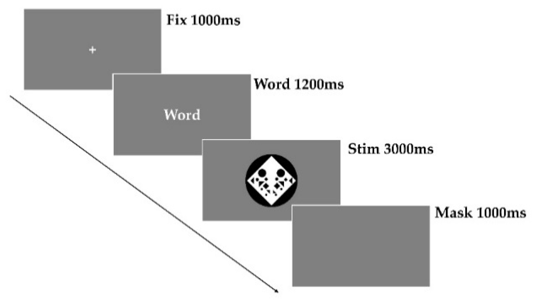
Figure 6.
Illustration of the stimulus paradigm applied.
Figure 6.
Illustration of the stimulus paradigm applied.
Before the main experiment, there will be a training block containing 20 stimuli (5 stimuli of each category), aiming to familiarize the participants with the experimental process. The stimulus materials in the training block will not appear in the formal experiment. Only when the accuracy rate of the training block is greater than 80%, the participants will be allowed to enter the formal experiment. The main experiment consists of a total of 300 trials, including 75 balance, 75 imbalance, 75 beautiful, and 75 not beautiful trials. The main experiment is divided into three blocks, each with 100 trials, and there is at least a 5-minute break between each block. Each trial begins with a stationary white cross at the center of the screen, displayed on a gray background for 1000ms. Subsequently, a cue word (beauty, balance) for the judgment task is presented for 1200ms. After that, a stimulus image appears for 3000ms, during which the participants are required to make a judgment and press the button as promptly as possible. Finally, a blank stimulus lasting for 1000ms appears, and the participants can blink and rest during this stage. The entire experiment takes approximately 1.5-2 hours, including the preparation stage before the experiment.
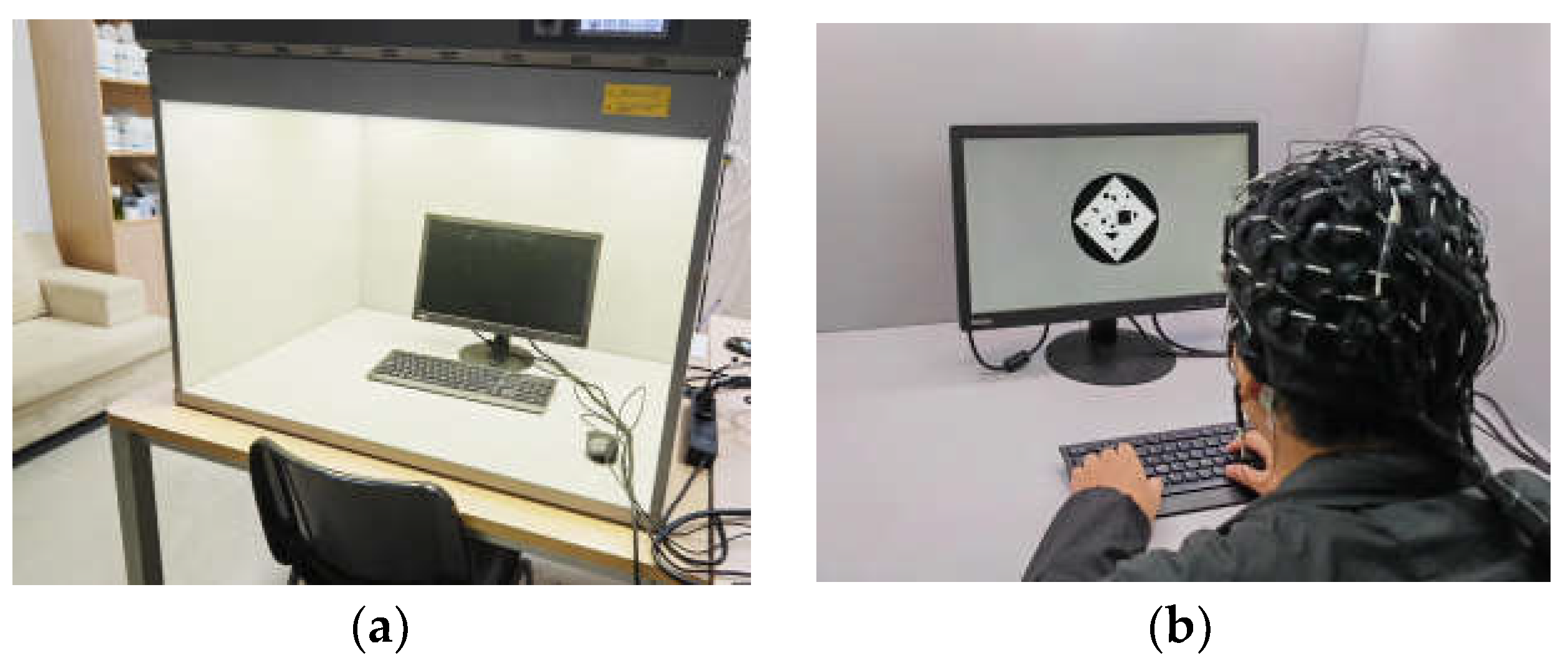
Figure 7.
Mian-experiment:(a) Display of the experimental environment.; (b) Participant Performing Binary Responses to Stimuli in the Main Experiment.
Figure 7.
Mian-experiment:(a) Display of the experimental environment.; (b) Participant Performing Binary Responses to Stimuli in the Main Experiment.
3. Results
EEG data were recorded using Neuroscan Synamp2 equipment. The reference electrodes were placed on both mastoids (M1, M2), and two pairs of electrodes were used to record the vertical electrooculogram (VEOG) and horizontal electrooculogram (HEOG). The VEOG electrodes were placed above and below the left eye, respectively, and the HEOG electrodes were placed 1 cm away from the outer corner of each eye. During the experiment, the impedance between the electrodes and the scalp was maintained below 10kΩ to ensure signal quality.
After the completion of continuous EEG recording, offline data processing was carried out. CURRY8.0 software was utilized to extract and analyze the EEG data. This included steps such as EEG data segmentation, artifact removal, baseline correction, and averaging. The bandpass filter range was set to 0-30 Hz, and the EEG artifact removal criterion was ±100μV. Subsequently, the EEG data were segmented into 1200ms epochs, with a time window ranging from 200ms before the stimulus onset to 1000ms after the stimulus onset, and the 200ms before the stimulus onset was used as the baseline. 60-channel data were used for repeated-measures Analysis of Variance (ANOVA). Mauchly's sphericity test and within-subject effects test were employed. Finally, Bonferroni's post hoc comparison method was used for multiple pairwise comparisons to explore specific differences between groups.
Since the EEG data of two participants were not satisfactory (availability rate < 50%), the data of 16 participants were retained for analysis (with an average of 6.7% of the data being rejected).
3.1. Behavioral Results
The effects of different tasks (aesthetic, balance) and different answers (yes, no) on the accuracy (ACC) and reaction time (RT) of judgment were analyzed using repeated measures ANOVA. The results revealed that the main effects of the answer and task factors on the ACC were not significant (F<1), and the interaction was also not significant [F (1, 15) = 3.956, p = 0.065]. It can be observed from the
Table 2 that the accuracy rates in all four conditions were greater than 90%, indicating that the participants were able to accurately discriminate whether the experimental materials were beautiful and whether the composition was balanced.
The main effects of task and answer on RT were not significant (F<1), but the interaction was significant [F (1, 15) = 4.952, p = 0.042]. Further analysis revealed that the specific results showed that there were no significant differences between answers under each task condition, and there were no significant differences between tasks under each answer condition. This suggests that the significance of the interaction may result from the small differences in specific condition combinations rather than the overall significant differences.
3.2. Event-Related Potential Results
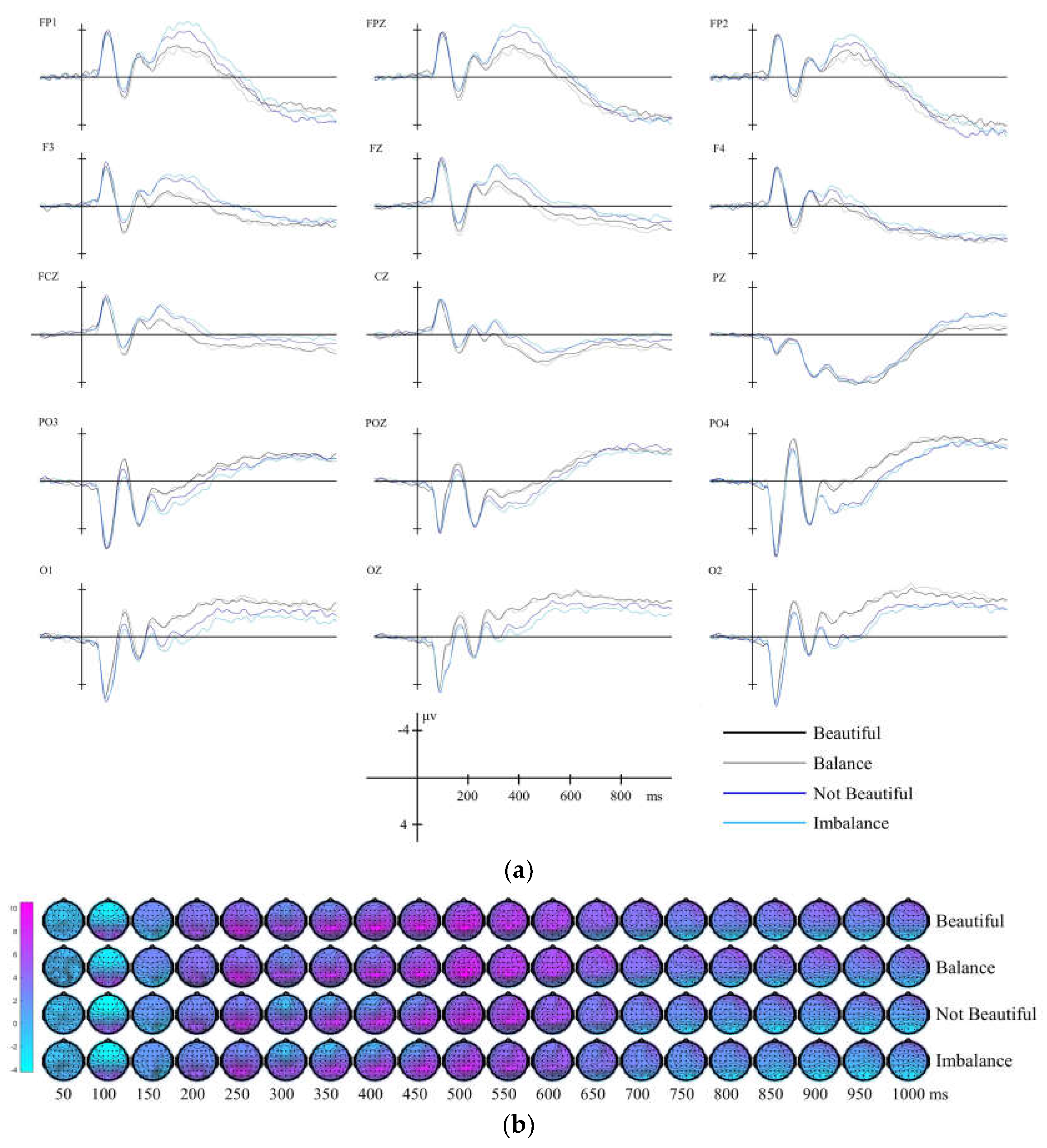
As shown in
Figure 8, the grand-average ERP and isopotential contour plot indicated that starting from 300ms to 500ms, a negative wave with a relatively larger amplitude was activated in the anterior frontal to central regions of the anterior half of the brain. In the parietal-occipital regions, different experimental conditions triggered positive waves with varying amplitudes. Within the time window between 600ms and 1000ms, distinct negative waves were activated in the parietal region under different experimental conditions.
3.2.1. Early Stage (300-500ms)
A three-factor repeated measures ANOVA was performed on the ERP average amplitude data across all electrodes using channel (60) × task (aesthetics, balance) × answer (Yes, No). The findings indicated: The task main effect was significant [F (1, 15) = 4.999, p = 0.041], with the average amplitude of the balance task (0.232μV±0.037) being notably smaller for the aesthetics task (0.256μV±0.034). The main effect of the answer was significant [F (1, 15) = 13.659, p = 0.002], with the average amplitude for the answer "Yes" (0.290μV±0.037) significantly greater than for the answer "No" (0.208μV±0.132). The interaction between channel and task was not significant [F (59, 885) = 1.210, p = 0.139]. The interaction between channel and answer was significant [F (59, 885) = 13.308, p<0.01]. Further analysis (
Table 3) revealed that in the prefrontal (FP1, FPZ, FP2), frontal lobe (F3, FZ, F4), and near the central region (FCZ, CZ, CPZ), the "No" answer condition activated a larger negative wave. In the parietal-occipital (PO3, POZ, PO4) and occipital regions (O1, OZ, O2), the average amplitude for the "No" answer was significantly greater than for the "Yes" answer, with the "No" condition activating a larger positive wave.
The three-way interaction was significant [F (59, 885) = 1.495, p = 0.011]. Further analysis (
Table 4) showed that in the prefrontal, frontal, and central regions, a larger negative wave was activated for the “No” answer in both tasks. In the parietal-occipital and occipital regions, a larger positive wave was activated under the “No” condition for both tasks.
3.2.2. Late Stage (600-1000ms)
A three-factor repeated measures ANOVA was performed on the data, yielding the following results: The main effect of the task was not significant (F<1). The main effect of the answer was significant [F (1, 15) = 4.906, p = 0.001], with the average amplitude for the answer "Yes" (0.191μV±0.027) significantly greater than for the answer "No" (0.119μV±0.034). The interaction between channel and task was not significant (F<1). The three-way interaction was not significant (F<1). The interaction between channel and answer was significant [F (59, 885) = 1.605, p = 0.003]. Further analysis (
Table 5) revealed that in the PZ channel, the main effect of the answer was significant [F (1, 15) = 5.196, p = 0.038], with the negative wave amplitude for the answer "Yes" (-0.143μV±0.446) being smaller than for the answer "No" (-0.806μV±0.411), particularly in the aesthetics task.
4. Machine Learning Model
Based on the experimental results, a model of the experimental data is constructed. On the one hand, this is to further verify the reliability of the experimental results, and on the other hand, it is to explore the feasibility of optimizing the model by increasing the data of neuroaesthetics research. This study involves the interaction of two tasks (aesthetics, balance) and two answers (Yes, No). Four types of data need to be classified, and the proportion of the four types of data is basically equal. Therefore, the support vector machine (SVM) is selected for modeling. SVM is a potent supervised learning model widely applied in classification and regression analysis. It achieves classification tasks by finding the optimal hyperplane to separate data samples of different categories. Its primary advantage lies in its ability to handle high-dimensional data [
48]. In this study, the LIBSVM toolbox is used to implement the training and prediction of the SVM model, and the LIBSVM supports multiple kernel functions (such as linear kernel, polynomial kernel) and multi-class classification tasks [
49]. Use the LIBSVM toolbox in MATLAB to train the data, select the appropriate penalty parameter C and kernel parameter γ, then train the SVM model with the best parameters, and evaluate the performance on the test set [
50].
First, based on the behavioral data, the data with incorrect judgments by the subjects were eliminated, and the experimental data with correct responses were retained, totaling 4548 groups. In the output layer data, the classification results of the stimulus materials' balanced composition were based on the results of the experimental calculation, and the aesthetic classification results of the stimulus materials were based on the classification results of each participant. The input layer data of the model included the feature data related to the balanced composition of the materials, and different schemes were selected for SVM modeling:
Scheme I: The input layer only contained the parameter data related to balanced composition in this study: symmetry, center of gravity, and negative space;
Scheme II: The input layer included the data in Scheme I, behavioral data (RT), and ERP data. The electrodes on the midline were selected, including the average amplitudes in the 300-500ms time window of the FPZ, FZ, FCZ, CZ, POZ, and OZ electrodes and the average amplitudes in the 600-1000ms time window of the PZ channel.
All data were standardized (standardization):
Here, is the standardized feature value, is the original feature value, is the mean of the feature, and is the standard deviation of the feature.
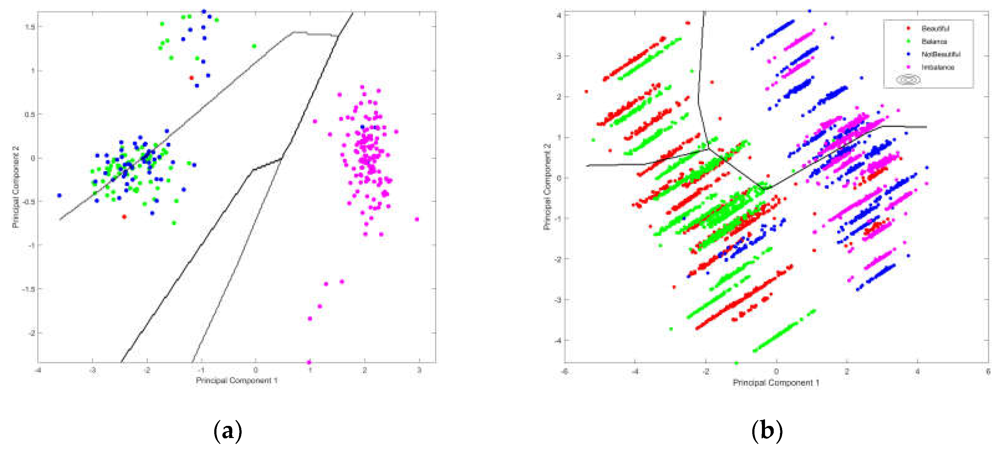
Next, determine whether the data is linearly separable in the original feature space. Use the Principal Component Analysis (PCA) method to reduce the dimensionality of the data set to 2 dimensions, train a simple linear classifier (C=1), and evaluate the performance of the linear classifier using 10-fold cross-validation. The results are shown in
Figure 9.
The decision boundary indicates that the decision boundaries of both schemes cannot effectively separate different categories of samples, with obvious intersections and overlaps, the model is not linearly separable in the reduced-dimensional feature space. Hence, the Radial Basis Function Kernel (RBF) is chosen for modeling. The RBF kernel function can map the original feature space to a high-dimensional feature space, enabling the data to be linearly separable in the new feature space, thereby addressing the issue of linear inseparability in the original feature space [
51,
52]. 80% of the data is utilized as the training set, and 20% of the data is used as the test set. The model quality is evaluated through 10-fold cross-validation, and the grid search method is employed to determine the optimal C and γ. In the preliminary search stage, 5 values are uniformly sampled within a large range [−2, 2] in the logarithmic space, and the ACC is used for comprehensive assessment. The results are presented in
Table 6:
The preliminary search results indicate that the C and γ of the two schemes perform well within the interval [0.01, 10]. Thus, in the fine search stage, the search range of C and γ is narrowed down to [0.01, 10], and 50 candidate values are generated using linear space sampling, totaling 25,000 combinations. To comprehensively evaluate the performance of the proposed model, the area under the receiver operating characteristic curve (AUC) is utilized to assess the performance of the multi-class SVM model. For the four-type classification problem in this study, and the macro-average method, which calculates the AUC value of each category and takes the average, is used to comprehensively evaluate the overall model performance. Through this approach, the classification ability of the model on different categories can be comprehensively understood, and the accuracy and reliability of the evaluation results can be ensured. The AUC threshold is set at 0.7, and on this basis, the SVM classification model with the highest ACC is sought to ensure that the model has strong discriminatory ability while maximizing its overall classification accuracy. The results are presented in
Figure 10 and
Table 7.
It can be seen from
Figure 10 and
Table 7 that the optimal solution of Scheme I has an average loss of 0.2932 in the model cross-validation, an accuracy rate of 0.7074 on the test set, and an AUC of 0.8822. The model has a certain classification ability. The optimal solution of Scheme II has an average loss of 0.003 in the cross-validation, an accuracy rate of 0.9989 on the test set, and an AUC of 0.9997. Compared with Scheme I, the classification effect of Scheme II is better, the performance of the model in different folds is relatively stable, and the performance on the training and validation sets is consistent, indicating that the model has good generalization ability. According to the display of precision, recall, and F1 value, Scheme II has a significant overall improvement in the classification ability of each category compared to Scheme I.
5. Discussion
In this study, the materials were classified into balanced and imbalanced compositions based on several parameters, including symmetry, center of gravity, and negative space. Behavioral data indicated that the participants were able to quickly and accurately categorize the materials only after receiving a brief introduction before the formal experiment to understand the characteristics of balanced compositions in this study. This further proves that people can quickly learn to understand and distinguish whether the composition of a picture is balanced [
13,
53]. After removing the experimental data with incorrect responses, a statistical analysis of the materials that the subjects considered beautiful and not beautiful revealed that 92.92% of the materials considered beautiful by the participants were balanced compositions, and 7.08% were imbalanced compositions, while 93.58% of the materials considered not beautiful were imbalanced compositions, and 6.42% were balanced compositions. In other words, during the pre-experiment, when the subjects were not informed of the purpose of the experiment, they mostly chose balanced compositions as the main criterion for evaluating beauty. This finding suggests that although a balanced composition does not always signify beauty, it is indeed one of the crucial factors in evaluating the aesthetic effects of images [
29,
30]. Moreover, balance serves as an important organizational design principle underlying the compositional strategies that adults employ when creating visual displays [
54].
ERP data revealed that in the early stage (300-500ms), ERP data showed significant separation between tasks, and the aesthetic task activated more extensive and active brain region activities than the balance task. At the same time, significant separation also occurred in the answers, and beautiful and balanced materials activated more active brain region activities in this time window. Specific analysis showed that unbeautiful and imbalanced materials activated significant ERP components in different brain regions: unbeautiful and imbalanced materials activated larger-amplitude negative waves in the prefrontal to central regions, and larger-amplitude positive waves in the parietal-occipital and occipital regions. In the late stage (600-1000ms), ERP data showed significant separation in the answers, specifically on the PZ channel, where beautiful materials activated a larger-amplitude Sustained Posterior Negativity (SPN).
Studies have demonstrated that the frontal lobe is closely associated with the process of emotional regulation, and the orbitofrontal cortex (OFC) exhibits distinct activities when perceiving beautiful and ugly stimuli. The OFC plays a crucial role in artistic creation and an individual's identification of the "beauty" in paintings [
55,
56,
57,
58]. There are significant differences in the ERP of the aesthetic response to artistic stimuli in the prefrontal region, and negative emotional stimuli (such as disgusting pictures) can trigger a larger-amplitude negative wave [
59,
60,
61]. Research has shown that early negative emotions are generated in the prefrontal cortex to evaluate unbeautiful patterns that form early impressions in the response. The early frontal negative wave reflects the processing stage involving negative aesthetic evaluation [
23,
62]. In the aesthetics task and balance task of this study, the unbeautiful and imbalanced stimuli activated a larger-amplitude frontal negative wave, indicating that the brain experienced higher cognitive conflict and emotional discomfort when confronted with these stimuli. Both aesthetics judgment and balance judgment have triggered a higher cognitive load and emotional response to stimuli that do not conform to expectations in cognitive processing, which is reflected in the enhancement of the frontal negative wave. This provides a neurophysiological basis for understanding the interaction between cognition and emotion in aesthetics and balance judgments.
The P300 component in the parietal-occipital region reflects the difference in attentional selection of target stimuli in different tasks and is closely related to the redistribution of attention [
63,
64,
65]. In the aesthetic task, the specific manifestation is that compared with less efficient processing, efficient processing is considered to result in a lower response [
66]. In this study, unbeautiful and imbalanced materials may attract more attentional resources, and beautiful stimuli usually trigger positive emotional responses. This emotional pleasure can reduce cognitive load, thereby reducing the amplitude of P300. Balanced compositions are typically regarded as stable and comfortable, and may induce less cognitive load. The larger-amplitude P300 component might reflect the brain's enhanced attention and concentration on these stimuli. Additionally, it suggests that when processing unbeautiful and imbalanced materials, more attentional resources are required to analyze and comprehend this visual information, resulting in increased processing difficulty and decreased sorting efficiency. This outcome implies that the characteristic of balance is closely associated with the connection between aesthetics and cognitive processing, and balance is a significant aspect of beauty.
The Sustained Posterior Negativity (SPN) is considered to be associated with the aesthetic judgment task and is predominantly observed in posterior brain regions such as the occipital and parietal lobes. It shows a continuous negative deflection, reflecting the cognitive activities and additional cognitive resources required in the process of visual attention and spatial processing. When a figure is considered beautiful, the emotional pleasure may ease the cognitive load, thereby reducing the SPN amplitude, which is considered to illustrate the importance of some features (such as symmetry) in aesthetic judgment [
67,
68,
69,
70,
71]. Herron's study discovered that the SPN in the 600-1200ms range is sensitive to task fluency. When the retrieval task is not fluent, the SPN amplitude is larger, and as task fluency increases, the SPN shows a graded attenuation [
72]. In this study, on the PZ channel, there was no significant difference in the SPN in the balance task, suggesting that although balance is also a visual aesthetic feature, its processing may differ from that of symmetry. Although the symmetrical feature is also a global composition feature, it typically has distinct visual cues, while the balance feature, especially asymmetric balance, requires the coordination of the overall layout and element distribution, which may result in the balance judgment task, regardless of whether it is balanced or imbalanced, the subjects analyzing all the elements in all the pictures, thus there is no obvious SPN difference However, in the aesthetic task, the beautiful stimulus activates a smaller-amplitude SPN, possibly because in the aesthetic task, the beautiful stimulus triggers a positive emotional response, reducing the brain's cognitive processing load on these stimuli, which is consistent with the emotion regulation theory and task fluency theory, that is, when the subjects encounter beautiful experimental materials, positive emotions can alleviate the cognitive load, and the processing process is smoother and easier.
The study demonstrates the effectiveness of integrating neuroaesthetic data and hand-crafted features in enhancing the performance of aesthetic evaluation models. By incorporating both behavioral and ERP data into the SVM model, Scheme II significantly outperformed Scheme I, which only utilized features related to balanced composition. Scheme II achieved a notably higher accuracy rate (0.9989) and AUC (0.9997), indicating superior classification capability and generalization ability. The inclusion of ERP data, specifically the average amplitudes in key time windows and channels, allowed the model to capture more nuanced patterns associated with aesthetic judgment. This implies that integrating human factors via an interdisciplinary approach which combines neuroaesthetics and advanced machine learning models can more effectively establish an integrated aesthetic evaluation system that can simulate and predict human aesthetic preferences [
43,
44,
73].
