
Submitted:
24 July 2024
Posted:
26 July 2024
You are already at the latest version
Abstract
Recently, flares have been considered as a major source of air pollution from the petroleum refining industry. The United Nations have instigated an international effort related to the management of flare emissions to reduce the global warming impact related to flaring. Eliminating or removing the need for gas flares is difficult because these devices are generally used as safety devices to allow combustion of flammable gases in a controlled fashion which supports safe operation. However, reducing flaring is generally possible using well designed efficiently operated flare equipment. In general, flare performance can be enhanced following the API-521 methodology and using assist- media including air and steam to achieve smokeless operation. This present work will discuss flare emissions in petroleum refining industry, and a method to manage flare emissions. Moreover, this work will discuss flare Combustion Efficiency (CE) and Distraction and Removal Efficiency (DRE) in terms of efficient flare operation. This work uses actual operating flare data, published previously, will be used in this work together with the CFD Code C3d. This code, developed at the USDOE Sandia National Laboratory is based on a standard LES methodology to conduct transient flare analysis is used to simulate flare operation to estimate flame shape and emissions produced. In this work, a new air-assisted flare tip design which uses the Coanda effect to improve flare operation was analysed. This new flare design reduces the emission rate that demonstrates the design effectiveness. The analysis considers a flare 1m high and (6") diameter in the centre of a 4m*4m*4m domain. Boundary conditions considering no cross wind and an ambient temperature of 300K. The initial condition is a hydrostatic pressure profile across the computational domain. In the air assist simulation, stoichiometric ratio will be a variable and therefore more than one case was considered.
Keywords:
CFD
; Gas Flare
; Soot Emissions
; CE
; DRE
1. Introduction
In petroleum industry, flares used to burn gases that cannot be processed or stored due to technical, economical and safety reasons. Generally, flares used to burn either large volumes of gases during start-up or shut-down process, or small amounts of gases during routine operation [1]. Flares used not only in petroleum industry but also in other industries, such as; sewage digester, ammonia fertilizer and coal gasification [1,2]. Recently, the carbon emissions produced from the flares’ operation considered as a major challenge to climate change [1,3,4]. The undesirable by-products from flares’ operation affect local population and the environment through noise, thermal radiation, smoke, and (NOx, SOx, soot, CO2 and CO) emissions. To reduce the impact of these by-products, flares design and operation should be according to standards [5].
Generally, the top oil producing countries are the main contributors to the increase in the flaring volume due the increase in oil production rates. Figure 1 shows the rate of flaring volume due to oil production. Moreover, Figure 2 shows the gas flaring volume in the top 10 country between 2012 and 2022. According to these data, Iraq is the second largest flaring country after Russia. This is related directly to oil production rate and improper flare design and operation. Figure 3 shows the correlation between oil production, flaring volume and intensity in Iraq between 2016 and 2022.
Flares’ performance usually measured using two important parameters; Combustion Efficiency (CE) and Destruction and Removal Efficiency (DRE) [712]. The first parameter, CE, measures the amount of CO2 produced due to complete combustion of the fuel, while, the second one, DRE, measures the amount of consumed original fuel converted to CO and CO2 [13,16]. According to studies, a good DRE indicates a flame stability [1317]. Moreover, factors like tip velocity and gas heating value affect flame stability. Usually, flares produce emissions under unstable operation conditions [18,19]. The combustion efficiency found also affected by flame lift-off when the tip velocity exceeds the burning velocity of the flare gas. USEPA recommended flare operation with tip velocity less than the maximum allowable tip velocity measured using tip diameter, the density of the flared vent gas and the air, combustion zone gas composition. Generally, the flame stability affects by factors such as; flammability limits, flame speed, cross wind speed and ignition temperature [1921]. Field observations observed high combustion efficiencies at high flow conditions [14,22] while low combustion efficiencies below 98-99% noticed by some field measurements at low flow conditions [2327]. Studies showed that several factors cause low combustion efficiencies at low flow conditions. For example, the velocity of vent gas and flammability of the vent gas mixture [28].
The current study tests a new air assisted flare tip design to enhance the performance by improving the CE and DRE, and reducing the soot formation and other greenhouse gases. The proposed idea includes 32 small pipes (1" ID) around the stack near the tip to inject air at high velocity toward the flame to achieve smokeless operation. The design also includes a curved surface (Coanda effect) in front of the air injectors to produce homogenous flow from all directions and entrain more air toward the flame. Figure 4 shows the proposed new air assisted flare tip design. The effect of air on combustion studied by considering three air flow rates with the same gas flow rate. These tests considered stoichiometric air fuel ratio of the combustion. Moreover, to show the relation between flare gas flow rate and soot formation, three gas flow rates tested and monitored using utility flare. The highest gas flow rate used in the air assisted flare tests due the high soot formation and to show the effect of air on combustion more clearly.
The principle of injecting a jet into the crossflow is observed in many applications; for example, combustion equipment, mixing tanks, quenching systems, and drying systems. The distribution of flow in the domain of crossflow was reported affected by many factors including jet geometry, jet exhaust velocity, and the characteristics of the crossflow and injecting fluids [29]. Both computational and experimental approaches have been used to study the effects of different factors on the flow properties of jet gas injected into crossflow [3034]. The Coanda effect can be explained as “when a jet of fluid is passed over a curved surface, it bends to follow the surface, entraining large amounts of air as it does so". In other words, the Coanda effect can be defined as the tendency of a fluid to attach to a nearby surface and stay attached to it even if the surface curves away from the direction of the initial jet [3538]. Coanda principle can be found in various natural and man-made examples (such as medicine, industrial processes, maritime technology, and aerodynamics) due to the improvement in turbulent levels and entrainment [37,38]. On the other hand, the major problem of the Coanda effect is the detachment of the jet flow due to high static pressure at the nozzle exit. Therefore, to prevent or delay this problem is through reducing the static pressure at the nozzle exhaust. For example, using a convergent-divergent nozzle can significantly lower the static pressure and solve the problem [39,40]. In petroleum industry, the Coanda principle has been used to improve flare operation by designing Coanda flares. Since the Coanda effect entrains large amounts of air, this kind of flare compared to other types produces higher combustion efficiency, better smokeless operation, and less thermal radiation. Furthermore, the Coanda principle has been also used in aircraft for thrust vectoring for short take-off and landing [4043].
2. Methodology
The methodology of this work include a real flare gas composition from the field with CFD code C3d to simulate the utility and air assisted flare cases.
2.1. Case Study
This study used flare gas composition of a utility flare from an oilfield in Iraq/ Kurdistan Region. The complete flare data and analysis can be found also in Maaroof et al work [5]. The original flare hydraulic limits were changed with a flare of dimeter and height 6" and 1m respectively. Moreover, the original gas flow rate was changed with different flow rates and cases and applied in absence of crosswind. Table 1 shows the gas composition used in this study.
2.2. Computational Fluid Dynamics (CFD) Simulation
In this study, C3d LES based on Computational Fluid Dynamics (CFD) code version 2-19-24 was used to simulate the utility and air assisted flare cases. In this study, more than six cases were simulated to study the flare performance and air assisted effect on operation; in addition to, mesh independence study. These include three cases for utility flare at difference gas flow rates 0.3kg/min, 0.36kg/min, and 0.42kg/min. Furthermore, for the air assisted cases, the highest gas flow rate from utility flare was applied with three different air flow rates within the limit of air/fuel stoichiometric ratio; 5.7kg/min, 6.6kg/min and 8.2kg/min.
2.2.1. CFD Code C3d
Generally, C3d is a computational fluid dynamic (CFD) and heat transfer computer code aimed at solving a wide range of heat transfer and fluid mechanics problems in cases involving fires and flares. The code includes several optional sub-models that help simulate radiation heat transfer, deposition, and aerosol transport, material decomposition, chemical reactions, and combustion [44]. The C3d code has been used in several previous works [45,46]. This code is based on a CFD tool originally known as ISIS-3d, and it has been validated and used for simulating pool fires to investigate the thermal performance of nuclear transport packages [47,49]. Originally, the code was developed at Sandia National Laboratory, and has been commercialized into a new CFD tool known as C3d to be used for analyzing the performance of large gas flare. In fact, C3d has been used previously for evaluating the performance of air-assisted flares, non-assisted (utility) flares, and large multipoint ground flares [44,50,52] with the combustion model expanded and approved for application and testing of typical flare gas (methane, propane, ethylene, xylene, ethane and propylene). Furthermore, C3d has been used for predicting flame shape and size, estimating the potential for smoking ignition behavior and estimating the radiation flux from the flame to surrounding objects. I code has also been used to analyze multi-point ground flares and air flow through the surrounding wind fence, and the resulting flame shape and height during maximum firing conditions. Also, the code has helped to evaluate the spacing between flare tips and rows to ensure adequate airflow to individual burners during operation to avoid smoking during maximum relief conditions [51]. Moreover, the code has been used to study the impact of using a continuous pilot compared to a discrete ignition system, whereas various ignition scenarios consider instantaneous ignition compared to delayed ignition [50].
2.2.2. LES Vs. RANS CFD
Studies showed that the traditional CFD simulation tools that use the Reynolds-Averaged Navier-Stock (RANS) approximations may not compute accurately the flare combustion efficiency. This is because of large-scale mixing resulting from vertical coherent structures in the flames are not easily reduced to a steady state condition provided by a typical RANS. Furthermore, in RANS, unsteady information (i.e., flame shape and instantaneous mixing) cannot be properly captured by time averaging the equations. Industrial flares operate in turbulent flow conditions, which include large disparity time and length scales. The smallest of these scales is set by viscosity and the biggest is on the order of flare tip diameter. Generally, the combustion is limited by mixing rates due to non-premixed combustion. There are numerous central reaction steps with hundreds of species with a wide range of reaction time scales involved in the detailed kinetic mechanism of chemical reactions. Both radiative and convective heat transfer accompany in the exothermic nature of the chemical reactions. These processes are closely coupled; for instance, the chemical reactions are affected by the turbulent mixing of air and combustion gas. The chemical reactions change the density and consequently the mixing intensity through turbulence. This occurs because the gas temperature changes with the chemical reactions as heat is generated. Resolving all the time and length scales in practical turbulent combustion applications is very difficult and mostly not possible even with supercomputers. Alternatively, capturing important features of the flame can be done by resolving large time and length scales, responsible for controlling dynamics, and using subgrid scale models for more homogenous smaller scales. It has been observed that the Large Eddy Simulation (LES) approach can more accurately simulate transient flare gas combustion compared to a RANS approach [50,51,52,53,54,55,56,57,58].
2.2.3. CFD Models
In this simulation, the governing equations are discretized using a finite volume approach with orthogonal Cartesian coordinates to make the discretization very similar to a finite difference approach. All vector quantities in a finite volume formulation such as momentum are defined at the cell interface and scalar variables such as pressure and temperature are defined at cell centers. The flow equations in the C3d code are solved using a compressible version of the pressure-based solution algorithm [44,59]. Furthermore, the Large Eddy Simulation (LES) formulation is used to model turbulence. In this simulation, used air is assumed to be incompressible with slight changes in temperatures. Moreover, the momentum equation used in this simulation is solved using a conservative form of the momentum flux vector ().
2.2.4. Computational Domain and Flare Model
The computational domain size used in this work were 4m height, 4m length, and 4m width. The height of the domain was on the z-axis and started from – 0.1 to 0 to specify a ground (dry sand) for the flare model, then from zero to 4m. The length of the domain was on the x-axis and started from – 2m to +2m. Finally, the width was defined on the y-axis and started from – 2m to +2 m. Both the x-axis and y-axis start from – 2m to +2m to define a center to locate the flare model. The flare model was 1m height and 0.1524m ID and 0.44m OD where built out of carbon steel using the C3d code modeler. Figure 5 shows the domain and flare mesh and size, and Figure 6 shows solid and mesh view of the flare model. Figure 6d shows the flow of the air through the coanda surface. The boundary conditions included: no cross-wind, hydrostatics pressure defined across the domain, and the flare exit as a 3-D pressure.
The total number of hexahedral cells for the utility flare and air assisted flares were 512,000 (808080) and 729,000 (909090) respectively. In the air assisted flare case, the mesh was very fine in the area between 0.8m and 1m with 171,500 hexahedral cells (707035), see Figure 6c, to capture the flow from the air pipes correctly. The grid has been refined using a higher number of cells to better capture the changes in the results and to confirm that the 512,000 cell (utility flare) and 729,000 cell (air assisted flare) simulation were sufficiently accurate. Figure 7 and Figure 8 are mesh independence study for the soot formation at sampling location 3.5m (see Figure 12) in case of the utility flare (0.42kg/min gas) and the air assisted flare (0.42kg/min gas and 5.7kg/min air). Generally, according to these figures, the increase in cell number (refining the mesh) gives almost the same results in both cases.
2.2.5. Physical Model
In this simulation, the LES turbulence model was used to simulate fluid flow. Radiation effects were included in the energy equation. To keep monitoring the fuel distribution and concentration, soot, intermediate species, and products of combustion (H2O and CO2), individual species equations were also solved. The combustion model used for providing the sink and source terms for the species equations as a function of local gas temperature, species concentrations and turbulent diffusivity. The code predicted the flame emissivity using a series of models as a function of soot volume fraction, molecular gas composition, flame size, flame shape and combustion effluent temperature profile. These variables depend on solutions of the momentum, mass, species, and energy equations. In this simulation, radiation transport model used for predicting the radiation flux from the flame to external ground, as well as providing sink and source terms for the energy equation to predict the flame temperature distribution.
2.2.6. Chemical and Soot Model
The rate of combustion equations is defined by a combination of Arrhenius & Eddy breakup reaction time scales.
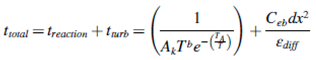
Ak is the pre-exponential coefficient, T is the local gas temperature, b is a global exponent, TA is activation temperature, Ceb is the eddy breakup scaling factor, dx is the characteristic cell size, εdiff is the eddy diffusivity from LES module, tturb is the turbulence time scale [44].
The combustion chemistry includes primary fuel breakdown reactions (incomplete combustion) that produce intermediate combustion products (C2H2, H2, CH4, Soot, and CO). Next, the reactions include burning the intermediate products and produce soot. Furthermore, reforming reactions with OH radicals are included, and the oxidizing species are simplified as water vapor. Equilibrium reactions between methane, acetylene, hydrogen, hydrogen sulfide and sulfur are included to allow to form soot [44]. The primary fuel breakdown reactions in this study are shown below:
CH4 + O2→ H2 + CO + H2O C1 Breakdown
C2H6 + O2→ 2.5H2O + 0.5C2H2 + CO C2 Breakdown
C3H8 + 1.5O2→ C2H2 + 2H2O + CO + H2 C3 Breakdown
C6H14 + 3.5O2→ 5H2O + 2C2H2 + 2CO C6+ Breakdown
H2S + O2– > SO2 +H2 H2S Breakdown
The secondary reactions of the gas are shown below:
H2 + 0.5O2→ H2O H2 combustion
C2H2 + 0.8O2→ 1.6CO + H2 + 0.02C20 soot nucleation soot formation
C2H2 + 0.01C20→ H2 + 0.11C2 soot growth by acetylene addition
CO + 0.5O2→ CO2 + H2O CO combustion
C20 + 10O2→ 20CO soot combustion
C2H2 + 3H2→ 2CH4 acetylene decomposition
CH4 + CH4→ C2H2 + 3H2 acetylene formation
0.5S2 + H2→ H2S sulfur reduction to hydrogen sulfide
H2S→1.5S2 + H2 hydrogen sulfide decomposition
H2S + 0.5SO2→ 0.75S2 + H2O elemental sulfur formation
The reforming reactions are showing below:
C20 + 20H2O→ 20CO + 20H2 soot steam reforming
0.75S2 + H2O→ H2S + 0.5SO2 sulfur steam reforming
For these reactions, a global Arrhenius rate mode is used. The consumption of soot, fuel and intermediate species are described by:
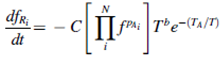 where N = number of reactants, fRi = moles of each reactant, i and C = pre-exponential coefficient, TA = effective activation temperature and b = temperature exponent.
2.3. Post Processing and Transient Calculation
At the beginning, the simulation run for 100 timesteps to calibrate the gas and air mass flow rate injected through the small pipes (air injectors) and the flare. After this step, the simulation timesteps and time set to 1000000 step and 10 s, respectively to allow the process to stabilize. The net reaction energy source and timesteps for the utility and air assisted flare case (see Figure 9) shows the simulation reach stability after 2s.
3. Results
Paraview version (5.11.2) was used to visualize the flame size and shape, and also to extract mass fractions of the combustion products and soot formation in the domain using probe feature.
3.1. Flame Size and Shape
The CFD code C3d was used to give an estimation and imagination about the flame size and shape for both utility and air assisted flare cases. Three gas flow rates were used in the utility flare; 0.3kg/min, 0.36kg/min and 0.42kg/min to show the relation between case rate and emission quantity. Figure 10 shows the utility flare operation at three different gas rates.
These rates were chosen after testing many cases with different rates lower than these rates. Less than the minimum gas rate 0.3kg/min cause flame back flow issue. In other words, these rate are the minimum purge rate for the case study gas mixture. To explain this more, the gas mixture has a density of about 0.78kg/m3 and air density is about 1.225kg/m3, this mean at low flow rate, the gas density will face a phenomena called Rayleigh–Taylor instability. This issue happens when a lighter fluid tries to push heavier fluid [60]. Alhameedi et al [61] used also six-inch pipe but with propane as a flare gas, and lower flow rates than what were used in this study. This is again because the propane density is about 1.808kg/m3, which is higher than the air density; therefore, the low flow rate will not cause density instability and back flow issue.
Moreover, the highest flow rate in the utility case was chosen to study the effect of the air assisted flare on flame stability and combustion emissions since burning more gas will produce more emissions. Figure 11 compares the utility flare operation with the new air assisted flare design using the same amount of the gas 0.42kg/min and three air rates; 5.7kg/min, 6.6kg/min and 8.2kg/min. The air assisted flare affect the flame by consuming more fuel since more air will be available to react with the fuel in complete combustion reaction. In other words, air assisted flare destroy more fuel compared to utility flare. This is clear from the flame size, as the air rate increases the flame size decreases. The amount of air used in the air assisted flare was calculated based on stoichiometric air fuel ratio. Since natural gas with more than one composition was used as a gas in this study, three rates of air were applied after calculating the mixture stoichiometric air fuel ratio.
3.2. Combustion Products
Probe function in paraview was used to extract data of combustion products in the plume to evaluate the utility flare operation and study the effectiveness of the new air assisted flare. Two locations in the domain 3m and 3.5m near the plume were defined to locate the probes and record the data. The radius of each probe was 3" to cover as much as possible of the plume. Moreover, each probe was recoding the data in ten different locations around the probe to cover as much as possible of the plume from all directions. Figure 12 shows the probe location and height from the plume.
3.3. Soot Formation
The soot formation in both utility and air assisted flares were studied and demonstrated using Paraview and the CFD code. The soot formation in the utility cases show that as gas rate increases the soot formation increases too. This is due to the fact that more fuel will need more air to achieve complete combustion and in the lack of the required air, part of the fuel will convert to soot. Figure 13 shows the soot formation in the three utility flare cases.
The effectiveness of the new air assisted flare tip design on reducing the environmental pollution appears in the change of the soot formation rate compared to utility flare. Figure 14 compares the soot formation between utility and the new air assisted flare. As mentioned before, the highest gas rate in the utility flare was used to study the effect of the new tip so the effectiveness of the new flare tip will be clearer in controlling the pollution. The differences between the utility and air assisted flare soot formation is clear because the amount of air introduced in the assisted flare is enough for burning almost all fuel and reducing the smoke rate. The new flare tip design showed the ability to direct the flow toward the flame efficiently, and the coanda surface represented by the curve surface in the tip has the ability to keep the air attached to the surface and ensure there is air from all directions. In other words, the coanda surface will make the air flow flatten and therefore it will be distributed equally from all sides around the flame.
Figure 15 and Figure 16 compare the soot formation of the utility and air assisted flares at 3m and 3.5m sampling locations. The soot formation results show clearly the effect of the new air assisted flare tip on managing pollution and improve the flare operation. At both sampling locations, the soot formation decreased significantly after applying the air assisted tip. This approve the efficiency of the new design in managing and controlling the emissions produced by the flares’ operation.
3.4. Combustion Efficiency (CE) and Destruction and Removal Efficiency (DRE)
The performance of the utility and air assisted flares was studied and compared using CE and DRE since these two factors determine the flare combustion quality. The DRE was calculated for the gas mixture and methane since the main compound in the gas mixture is the methane. The equation below have been used to calculate these two factors.
Table 6 and Table 7 show the CE, DRE and DRECH4 for the utility and air assisted flare cases at the two sampling locations. Generally, the DRE results of the air assisted flare are higher than utility flare as more air will consume (destroy) more fuel. Moreover, the DRECH4 of the air assisted flare are higher than the utility flare. The effect of the new air assisted flare tip on the DRE and DRECH4 shown clearly in the Figure 19, Figure 20, Figure 21 and Figure 22. Regarding the CE, the air assisted flare improved considerably the CE from about 70 % in the utility flare to over than 95 %. The difference between the utility and the new air assisted flares CE appear clearly in the Figured 17 and 18.
3.5. Soot Formation, CE and Fuel Carbon Balance
To study more the effect of the new air assisted flare on managing emission and improving flare operation, the change in soot formation and CE were investigated and compared for both utility and air assisted flares. Table 8 shows the soot formation and CE for both flare cases (utility and air assisted) at the sampling locations.
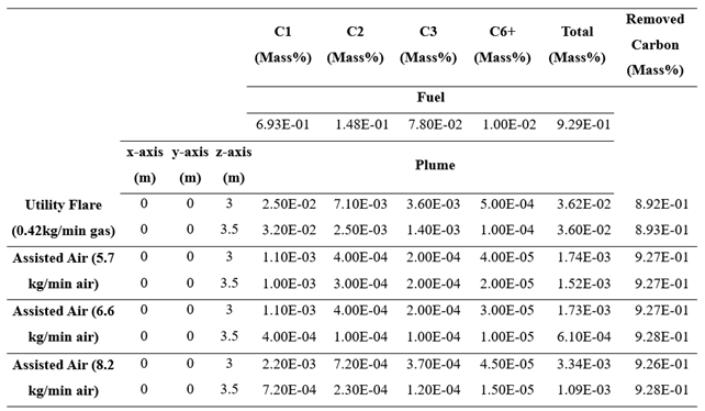
The fuel carbon balance shows the quantity of carbon removed from the fuel after combustion. This study compares the amount of C1, C2, C3 and C6+ in the fuel and the plume to understand the combustion more clearly. The original mass fraction of C1, C2, C3 and C6+ in the fuel compared to the plume shows a decrease in the amount of these compounds. The air assisted flare removed more of C1, C2, C3 and C6+ compared to the utility flare. This explain the DRE and combustion behavior of the air assisted flare. Table 9 shows the C1, C2, C3 and C6+ mass fraction in the fuel and the plume, and the amount of removed carbon due to combustion.
4. Conclusions
This paper studied the gas flare emission management using a new air assisted flare tip design. The CFD code C3d was used to simulate utility flare and air assisted cases at different flow rates. In this study, a utility flare gas composition from one of the oilfield in Iraq Kurdistan region was used as a flare gas in both utility and air assisted flare cases. Moreover, a flare hydraulic dimensions of 1m height and 6" inside diameter was used in this work. The new tip design included 32 small pipes of 1" ID distributed equally around the tip to inject air from all directions toward the flame. Moreover, the tip consisted of a curved surface to provide a conada effect to the air injected from the pipes. To understand the effect of the new tip design on managing and reducing the gas flare emissions, first a number of utility flare cases were simulated using three different gas flow rates to show the relation between the amount of gas burn and emission rates. Later, the highest gas flow rate was used in the air assisted flare simulation. After calculating the stoichiometric air fuel ratio, three rates of air within the limits of stoichiometric were applied in the simulation. The soot formation pictures showed the new air assisted flare tip design was able to reduce considerably the emission. Also, the thermal images showed that the air assisted flare was able to consume more fuel compared to the utility flare. The probe function in paraview was used to capture the product of combustion in the plume at two locations in the domain. The soot formation of the utility flare was significantly higher than the air assisted flare. Moreover, the performance of the new assisted flare tip design studied by considering the CE and DRE for both utility and air assisted flare. The results showed the assisted air flare improved the CE from around 70% to over 95%. Generally, the results showed that the new tip design was able to reduce and manage the gas emission produced by the gas flare.
References
- Emam, E.A. 2016. Environmental pollution and measurement of gas flaring. Int. j. innov. res. sci. eng. technol, 2, pp.252-262.
- Ling, A.L. 2007. Flare selection and sizing (engineering design guideline). KLM technology group, Malaysia.
- Evans, L.B.; Vatavuk, W.M.; Stone, D.K.; Lynch, S.K.; Pandullo, R.F. 2000. VOC Destruction Controls. North Carolina.
- Bahadori, A. 2014. Natural gas processing: technology and engineering design. Gulf Professional Publishing.
- Maaroof, A.A.; Smith, J.D.; Zangana, M.H. Design and simulation of a utility oilfield flare in Iraq/Kurdistan region using CFD and API-521 methodology. Heliyon 2023, 9, e18581. [Google Scholar] [CrossRef] [PubMed]
- World Bank [Online]. https://www.worldbank.org/en/programs/gasflaringreduction/global-flaring-data, 2024.
- Wood, E.C.; Herndon, S.C.; Fortner, E.C.; Onasch, T.B.; Wormhoudt, J.; Kolb, C.E.; Knighton, W.B.; Lee, B.H.; Zavala, M.; Molina, L.; et al. Combustion and Destruction/Removal Efficiencies of In-Use Chemical Flares in the Greater Houston Area. Ind. Eng. Chem. Res. 2012, 51, 12685–12696. [Google Scholar] [CrossRef]
- Allan, K. C. Combustion Efficiency of Full-Scale Flares Measured Using DIAL Technology. Alberta Research Council Inc., 250 Karl Clark Rd., Edmonton, Alberta, Canada.
- EPA, E. Enforcement targets flaring efficiency violations. Enforcement Alert, 10 (5), Aug. 2012. EPA 325-F-012-002.
- Johnson, M.R.; Zastavniuk, O.; Wilson, D.J.; Kostiuk, L.W. 1999. Efficiency measurements of flares in a cross flow.
- Johnson, M.R.; Majeski, A.J.; Wilson, D.J.; Kostiuk, L.W. 1998. The combustion efficiency of a propane jet diffusion flame in cross flow. Combustion and Environment Group, Department of Mechanical Engineering, University of Alberta.
- Joseph, D.; Lee, J.; McKinnon, C.; Payne, R.; Pohl, J. 1983. Evaluation of the Efficiency of Industrial Flares: Background- Experimental Design- Facility.
- Pederstad, A.; Smith, J.D.; Jackson, R.; Saunier, S.; Holm, T. 2015. Assessment of flare strategies, techniques for reduction of flaring and associated emissions, emission factors and methods for determination of emissions to air from flaring, Carbon Limits AS, Trondheim, Norway. Carbon Limits AS, Trondheim, Norway.
- Pohl, J.H.; Tichenor, B.A.; Lee, J.; Payne, R. 1986. Combustion efficiency of flares. Combustion science and technology, 50(4-6), pp.217-231.
- Pohl, J.H.; Soelberg, N.R. 1986. Evaluation of the efficiency of industrial flares: H/sub 2/S gas mixtures and pilot-assisted flares. Final report, April 1985-July 1986 (No. PB-87-102372/XAB). Energy and Environmental Research Corp., Irvine, CA (USA).
- Pohl, J.H.; Soelberg, N.R. 1985. Evaluation of the efficiency of industrial flares: Flare head design and gas composition.
- Standard, A.P.I. 2014. Pressure-relieving and depressuring systems. American Petroleum Institute, p.248.
- John Zink Company, SAFE FLARE SYSTEM DESIGN, 1993 [Online]. https://www.scribd.com/document/61112927/Flare-System. (Accessed 10 February 2024).
- Seebold, J.; Gogoloek, P.; Pohl, J.; Schwartz, R. ; 2004, October. Practical implications of prior research on today’s outstanding flare emissions questions and a research program to answer them. In AFRC-JFRC 2004 Joint International Combustion Symposium, Maui, HI.
- Aljerf, L.; AlMasri, N. Flame Propagation Model and Combustion Phenomena: Observations, Characteristics, Investigations, Technical Indicators, and Mechanisms. J. Energy Conserv. 2015, 1, 31–40. [Google Scholar] [CrossRef]
- Varner, V.; Fox, S.; Schwartz, R.; Wozniak, R. 2007. Pressure-assisted flare emissions testing. In American--Japanese Flame Research Committees International Symposium (pp. 1-12).
- McDaniel, M.; Tichenor, B.A. 1983. Flare efficiency study.
- Strosher, M.T. Characterization of Emissions from Diffusion Flare Systems. J. Air Waste Manag. Assoc. 2000, 50, 1723–1733. [Google Scholar] [CrossRef] [PubMed]
- Mellqvist, J. Flare testing using the SOF method at Borealis Polyethylene in the summer of 2000. Chalmers University of Technology. 2001. http://www. fluxsense. se/reports/flarepaperfinal, 201004.
- Maaroof, A.A.; Smith, J.D.; Zangana, M.H. Coanda effect enhanced air assisted flare for low flow operation: cold flow CFD analysis.
- Cade, R.; Evans, S. 2010. Performance test of a steamassisted elevated flare with passive FTIR. Chicago, Illinois: Clean Air Engineering.
- Ewing, B.; Roesler, D.; Evans, S. 2010. Performance Test of a Steam-Assisted Elevated Flare with Passive FTIR-Detroit. Final Report. Detroit: Marathon Petroleum Company, LP & Clean Air Engineering.
- Torres, V.M.; Herndon, S.; Kodesh, Z.; Allen, D.T. Industrial Flare Performance at Low Flow Conditions. 1. Study Overview. Ind. Eng. Chem. Res. 2012, 51, 12559–12568. [Google Scholar] [CrossRef]
- Alhameedi, H.A.; Hassan, A.A.; Smith, J.D.; Al-Dahhan, M. Toward a Better Air-Assisted Flare Design for Purge Flow Conditions: Experimental and Computational Investigation of Radial Slot Flow into a Crossflow Environment. Ind. Eng. Chem. Res. 2021, 60, 2634–2641. [Google Scholar] [CrossRef]
- Liscinsky, D.S.; True, B.; Holdeman, J.D. Crossflow mixing of noncircular jets. J. Propuls. Power 1996, 12, 225–230. [Google Scholar] [CrossRef]
- Kartaev, E.; Emelkin, V.; Ktalkherman, M.; Aulchenko, S.; Vashenko, S. Upstream penetration behavior of the developed counter flow jet resulting from multiple jet impingement in the crossflow of cylindrical duct. Int. J. Heat Mass Transf. 2018, 116, 1163–1178. [Google Scholar] [CrossRef]
- Elattar, H.F.; Fouda, A.; Bin-Mahfouz, A.S. CFD modelling of flow and mixing characteristics for multiple rows jets injected radially into a non-reacting crossflow. J. Mech. Sci. Technol. 2016, 30, 185–198. [Google Scholar] [CrossRef]
- Kartaev. ; Emel’kin, V.; Ktalkherman,.; Kuz’min, V.; Aul’chenko, S.; Vashenko, S. Analysis of mixing of impinging radial jets with crossflow in the regime of counter flow jet formation. Chem. Eng. Sci. 2014, 119, 1–9. [Google Scholar] [CrossRef]
- Nada, S.; Fouda, A.; Elattar, H. Parametric study of flow field and mixing characteristics of outwardly injected jets into a crossflow in a cylindrical chamber. Int. J. Therm. Sci. 2016, 102, 185–201. [Google Scholar] [CrossRef]
- Coanda, H. "Procédé de propulsion dans un fluide." Brevet Invent. Gr. Cl 2 (1932).
- Reba, I. Applications of the Coanda Effect. Sci. Am. 1966, 214, 84–92. [Google Scholar] [CrossRef]
- Lubert, C. On Some Recent Applications of the Coanda Effect. Int. J. Acoust. Vib. 2011, 16. [Google Scholar] [CrossRef]
- Wille, R.; Fernholz, H. Report on the first European Mechanics Colloquium, on the Coanda effect. J. Fluid Mech. 1965, 23, 801–819. [Google Scholar] [CrossRef]
- Parsons, C. 1990. An experimental and theoretical study of the aeroacoustics of external-Coanda gas flares.
- Carpenter, P.W. 1997. The Aeroacoustics and Aerodynamics of High-speed Coanda Devises. In The Seventh Asian Congress of Fluid Mechanics, 1997 (Vol. 8, No. 12, pp. 199-202).
- Castaneda, V.; Valera-Medina, A. Coanda flames for development of flat burners. Energy Procedia 2019, 158, 1885–1890. [Google Scholar] [CrossRef]
- Desty, D.H.; Boden, J.C.; Witheridge, R.E. 1978, June. The origination, development and application of novel premixed flare burners employing the Coanda effect. In 85th National AIChE Meeting, Philadelphia.
- Valera-Medina, A.; Baej, H. Hydrodynamics During the Transient Evolution of Open Jet Flows from/to Wall Attached Jets. Flow, Turbul. Combust. 2016, 97, 743–760. [Google Scholar] [CrossRef]
- Suo-Anttila, A. 2019. C3D Theory and User Manual.
- Smith, J.D.; Suo-Ahttila, A.; Smith, S.; Modi, J. 2007. Evaluation of the Air-Demand, Flame Height, and Radiation from low-profile flare tips using ISIS-3D. In American–Japanese Flame Research Committees International Symposium.
- Smith, J.D.; Al-Hameedi, H.A.; Jackson, R.; Suo-Antilla, A. Testing and Prediction of Flare Emissions Created during Transient Flare Ignition. Int. J. Petrochem. Res. 2018, 2, 175–181. [Google Scholar] [CrossRef]
- Suo-Anttila, A.; Wagner, K.C.; Greiner, M. Analysis of Enclosure Fires Using the Isis- 3D™ CFD Engineering Analysis Code. In Proceedings of the International Conference on Nuclear Engineering, January 2004; Volume 46881, pp. 721–730. [Google Scholar]
- Lopez, C.; Suo-Anttila, A.J.; Greiner, M.; Are, N. 2004. Effect of small long-duration fires on a spent nuclear fuel transportation package (No. SAND2004-3309C). Sandia National Laboratories (SNL), Albuquerque, NM, and Livermore, CA (United States).
- Greiner, M.; Suo-Anttila, A. Radiation Heat Transfer and Reaction Chemistry Models for Risk Assessment Compatible Fire Simulations. J. Fire Prot. Eng. 2006, 16, 79–103. [Google Scholar] [CrossRef]
- Greiner, M.; Suo-Anttila, A. Validation of the Isis-3D Computer Code for Simulating Large Pool Fires Under a Variety of Wind Conditions. J. Press. Vessel. Technol. 2004, 126, 360–368. [Google Scholar] [CrossRef]
- Smith, J.; Suo-Anttila, A.; Philpott, N.; Smith, S. 2010, September. Prediction and Measurement of Multi-Tip Flare Ignition. In American Flame Research Committees-International Pacific Rim Combustion Symposium, Advances in Combustion Technology: Improving the Environment and Energy Efficiency (pp. 26-29).
- Smith, J.; Jackson, R.; Suo-Anttila, A.; Hefley, K.; Smith, Z.; Wade, D.; Allen, D.; Smith, S. 2015. Radiation effects on surrounding structures from multi-point ground flares. In AFRC 2015 industrial combustion symposium (pp. 9-11).
- Smith, J.; Adams, B.; Jackson, R.; Suo-Anttila, A. 2017. Use of RANS vs LES Modelling for Industrial Gas-fired Combustion. Industrial Combustion.
- Smith, J.; Adams, B.; Jackson, R.; Suo-Anttila, A. 2017. Use of RANS and LES Turbulence Models in CFD Predictions for Industrial Gas-fired Combustion Applications. Journal of the International Flame Research Foundation.
- Evans, L.B.; Vatavuk, W.M.; Stone, D.K.; Lynch, S.K.; Pandullo, R.F. 2000. VOC Destruction Controls. North Carolina.
- Said, R.; Garo, A.; Borghi, R. Soot formation modeling for turbulent flames. Combust. Flame 1997, 108, 71–86. [Google Scholar] [CrossRef]
- Majeski, A.J.; Wilson, D.J.; Kostiuk, L.W. 1999. Size and trajectory of a flare in a cross flow.
- Torres, V.M.; Herndon, S.; Wood, E.; Al-Fadhli, F.M.; Allen, D.T. Emissions of Nitrogen Oxides from Flares Operating at Low Flow Conditions. Ind. Eng. Chem. Res. 2012, 51, 12600–12605. [Google Scholar] [CrossRef]
- Issa, R. Solution of the implicitly discretised fluid flow equations by operator-splitting. J. Comput. Phys. 1986, 62, 40–65. [Google Scholar] [CrossRef]
- Piriz, A.R.; Cortazar, O.D.; Lopez Cela, J.J.; Tahir, N.A. 2006. The rayleigh-taylor instability. American journal of physics, 74(12), pp.1095-1098.
- Alhameedi, H.A.; Smith, J.D.; Ani, P.; Powley, T. Toward a Better Air-Assisted Flare Design for Safe and Efficient Operation during Purge Flow Conditions: Designing and Performance Testing. ACS Omega 2022, 7, 42793–42800. [Google Scholar] [CrossRef] [PubMed]
Figure 1.
Global Gas Flaring and Oil Production Between 1996 and 2022 [5].
Figure 1.
Global Gas Flaring and Oil Production Between 1996 and 2022 [5].
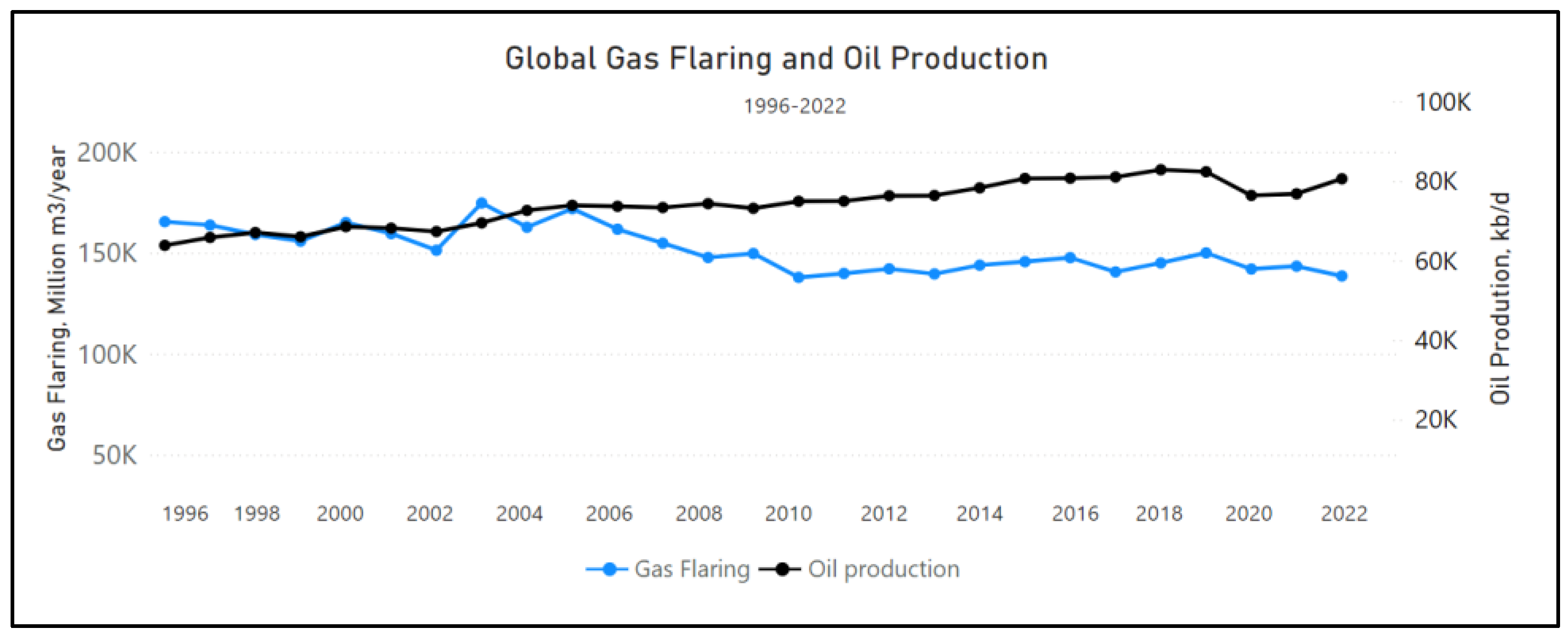
Figure 2.
Top Ten Flaring Countries (2012-2022) [5].
Figure 2.
Top Ten Flaring Countries (2012-2022) [5].
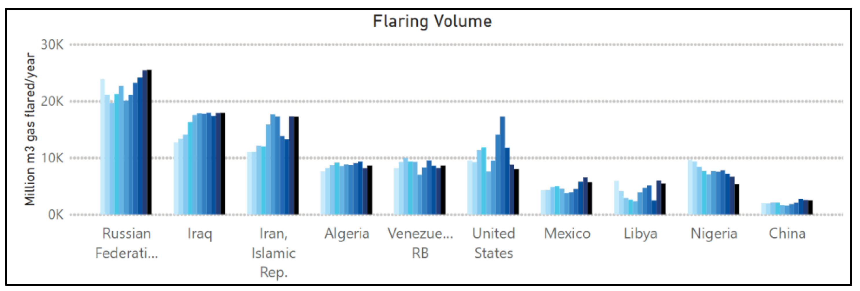
Figure 3.
Relation between flaring volume, flaring Intensity and oil production in Iraq (2016-2022) [5].
Figure 3.
Relation between flaring volume, flaring Intensity and oil production in Iraq (2016-2022) [5].
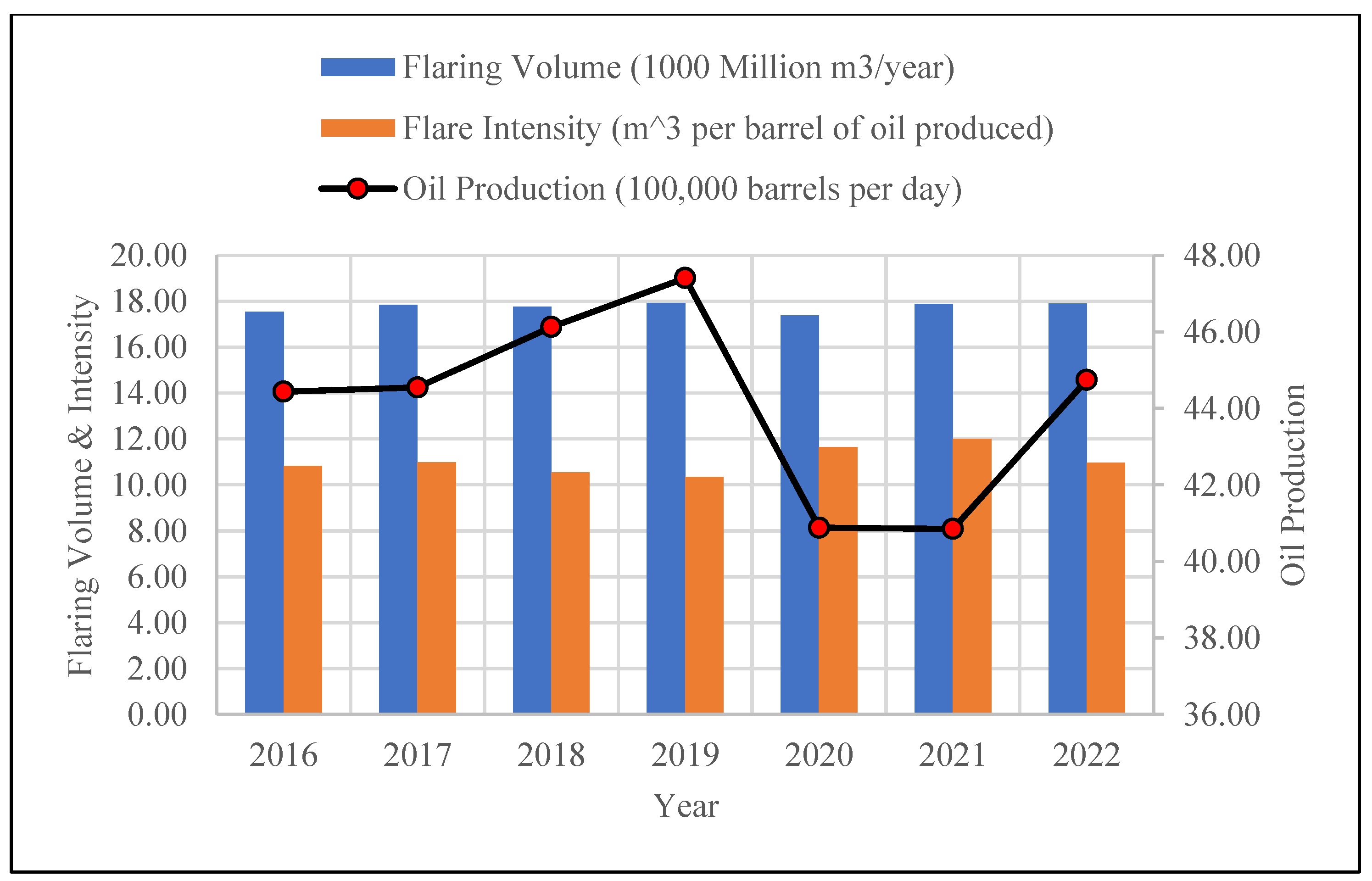
Figure 4.
The new air assisted flare tip design; (a) Side view, (b) Cross sectional view, (c) Tip cross sectional view, (d) Top view.
Figure 4.
The new air assisted flare tip design; (a) Side view, (b) Cross sectional view, (c) Tip cross sectional view, (d) Top view.
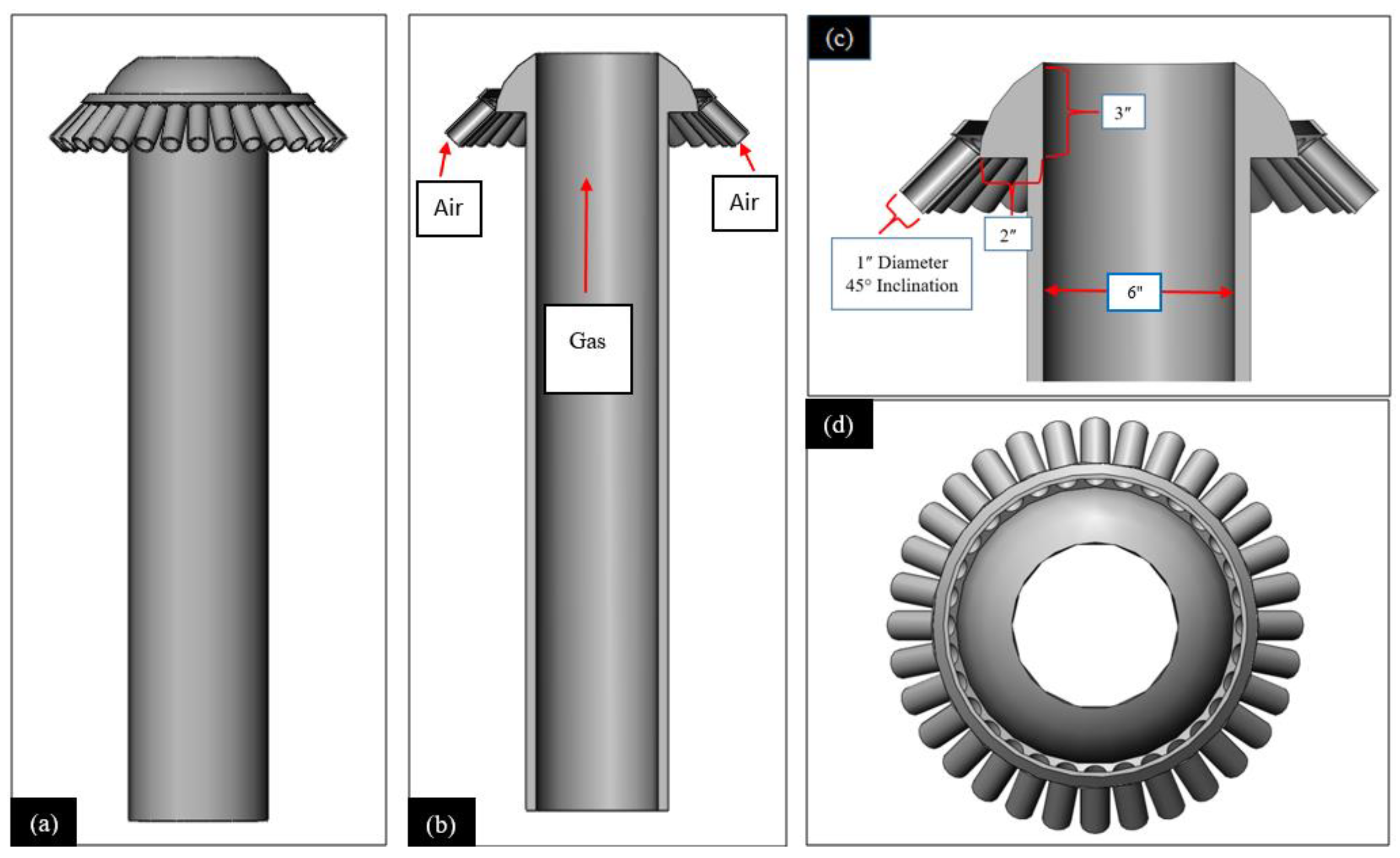
Figure 5.
CFD domain mesh and size; (a) Utility flare case, (b) Air assisted flare case.
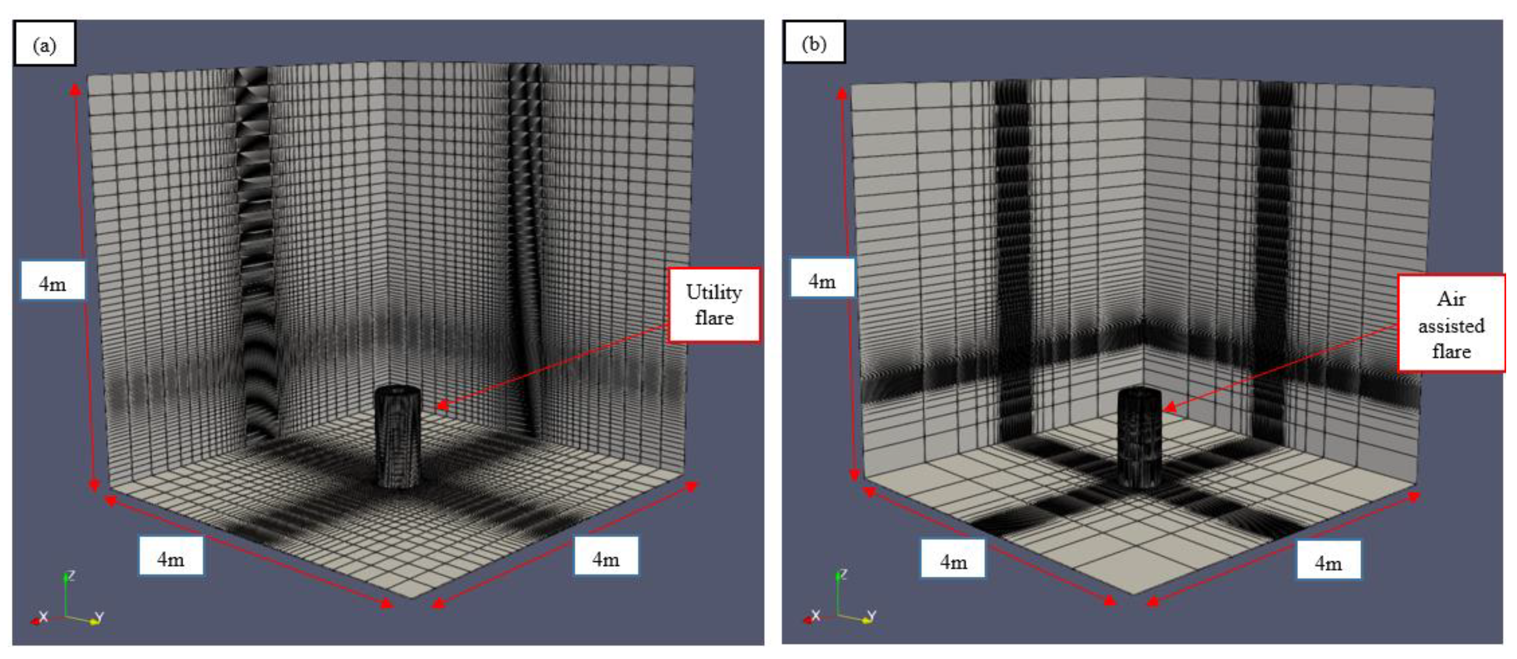
Figure 6.
Flare CFD model and mesh; (a) Cross sectional view, (b) Model meshing, (c) Tip meshing, (d) Cold flow (air flow).
Figure 6.
Flare CFD model and mesh; (a) Cross sectional view, (b) Model meshing, (c) Tip meshing, (d) Cold flow (air flow).
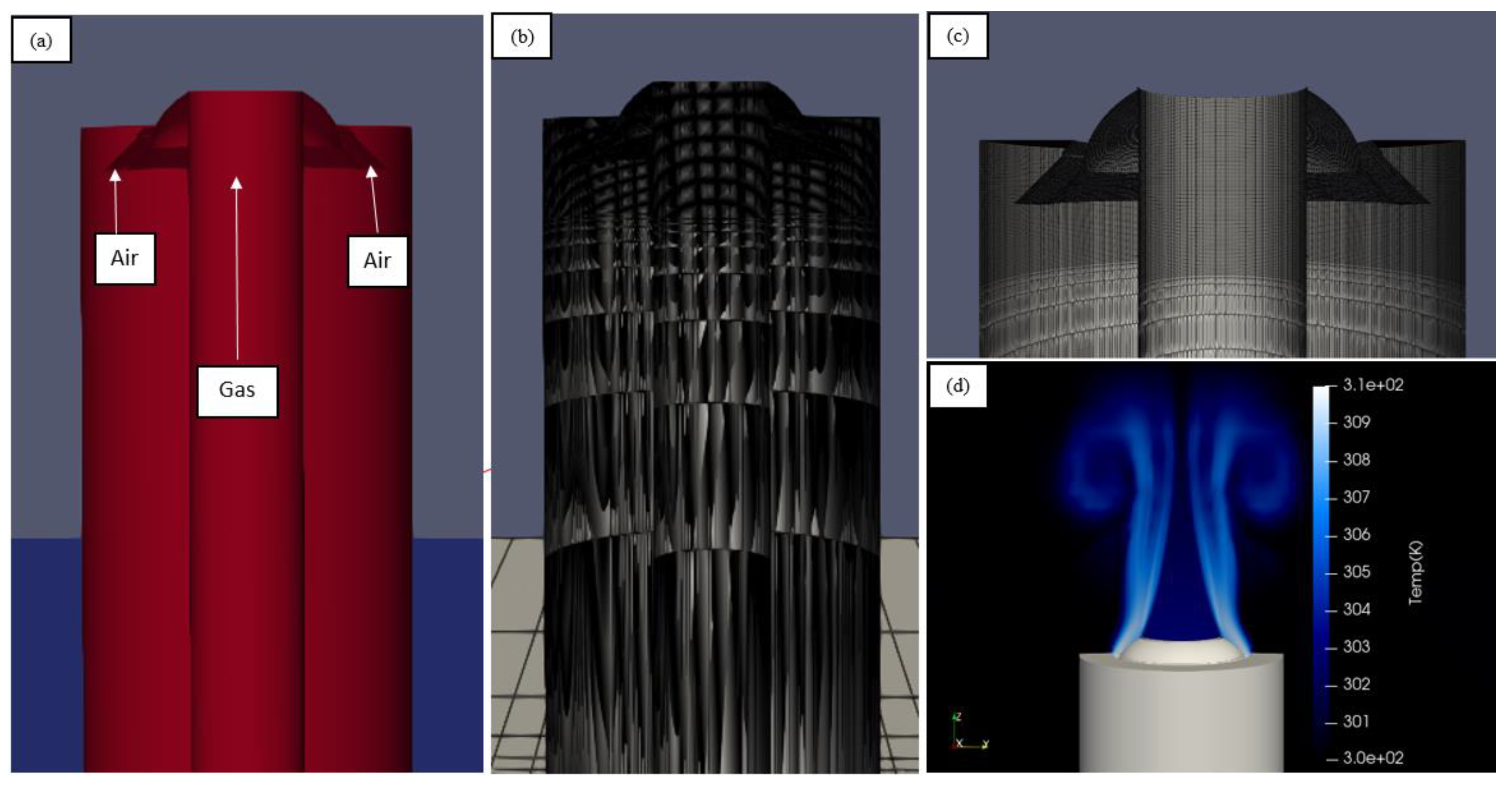
Figure 7.
Mesh independence study for air assisted flare case (0.42kg/min gas and 5.7kg/min air) at location 3.5m sampling point.
Figure 7.
Mesh independence study for air assisted flare case (0.42kg/min gas and 5.7kg/min air) at location 3.5m sampling point.
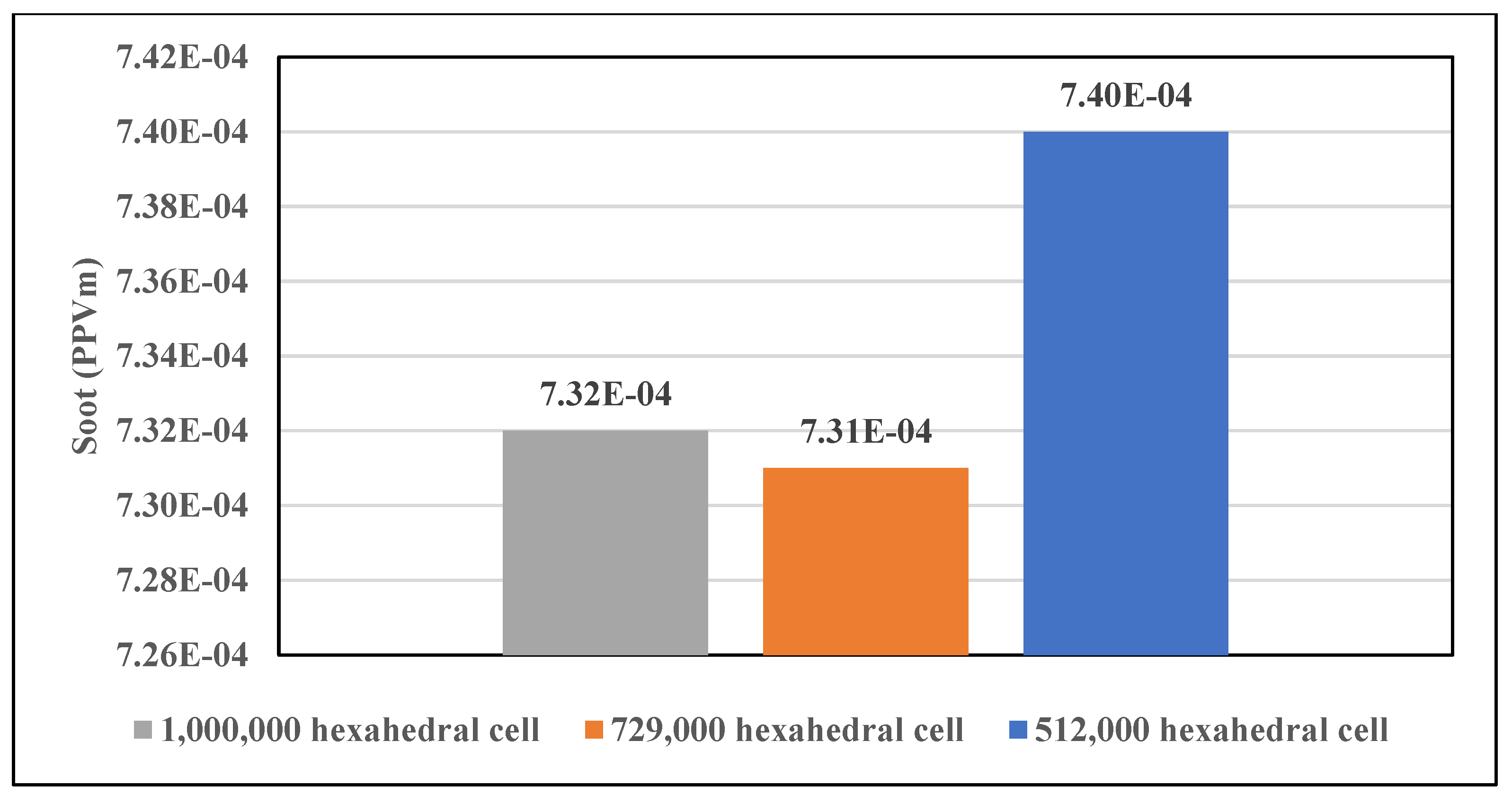
Figure 8.
Mesh independence study for utility flare case (0.42kg/min gas) at location 3.5m sampling point.
Figure 8.
Mesh independence study for utility flare case (0.42kg/min gas) at location 3.5m sampling point.
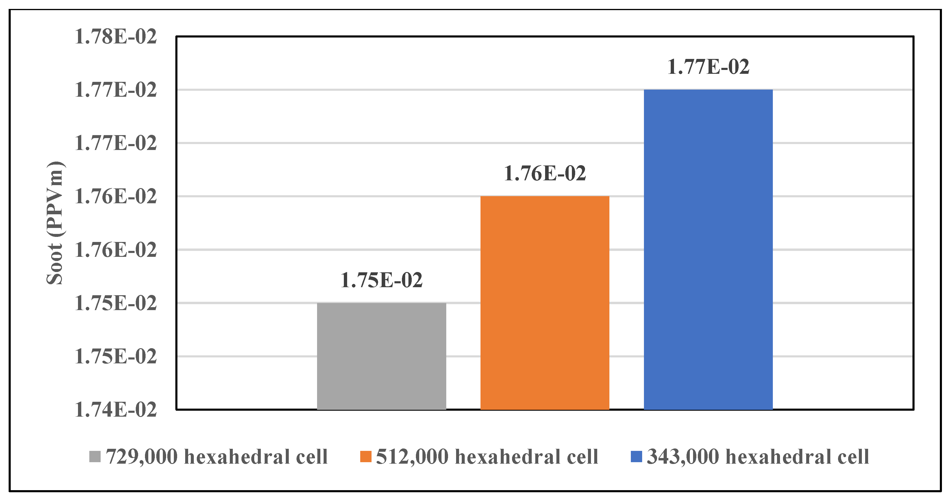
Figure 9.
Utility and air assisted flare Cases’ simulation stability.
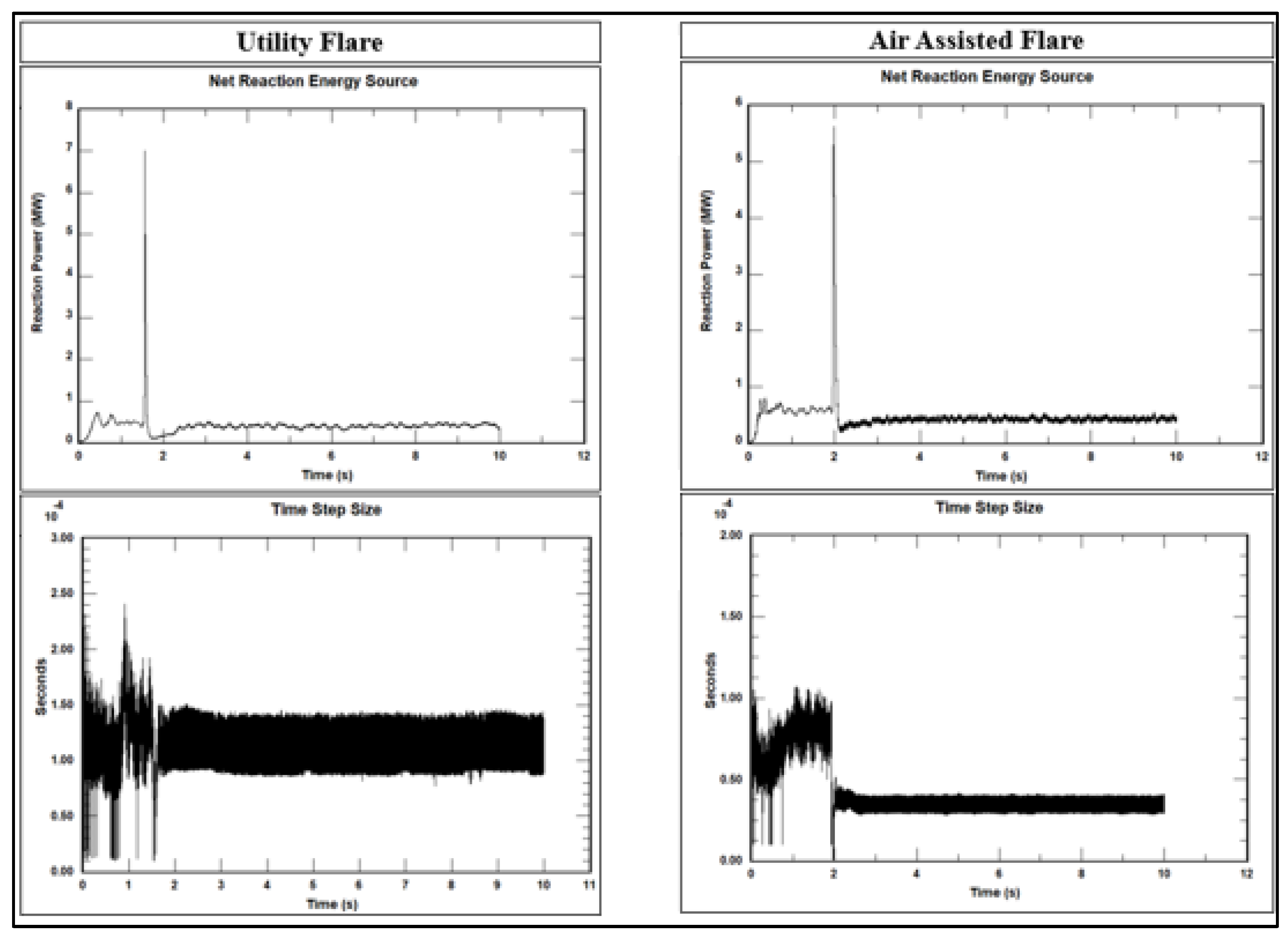
Figure 10.
Utility flare cases; (a) 0.3kg/min gas, (b) 0.36kg/min gas, (c) 0.42kg/min gas.
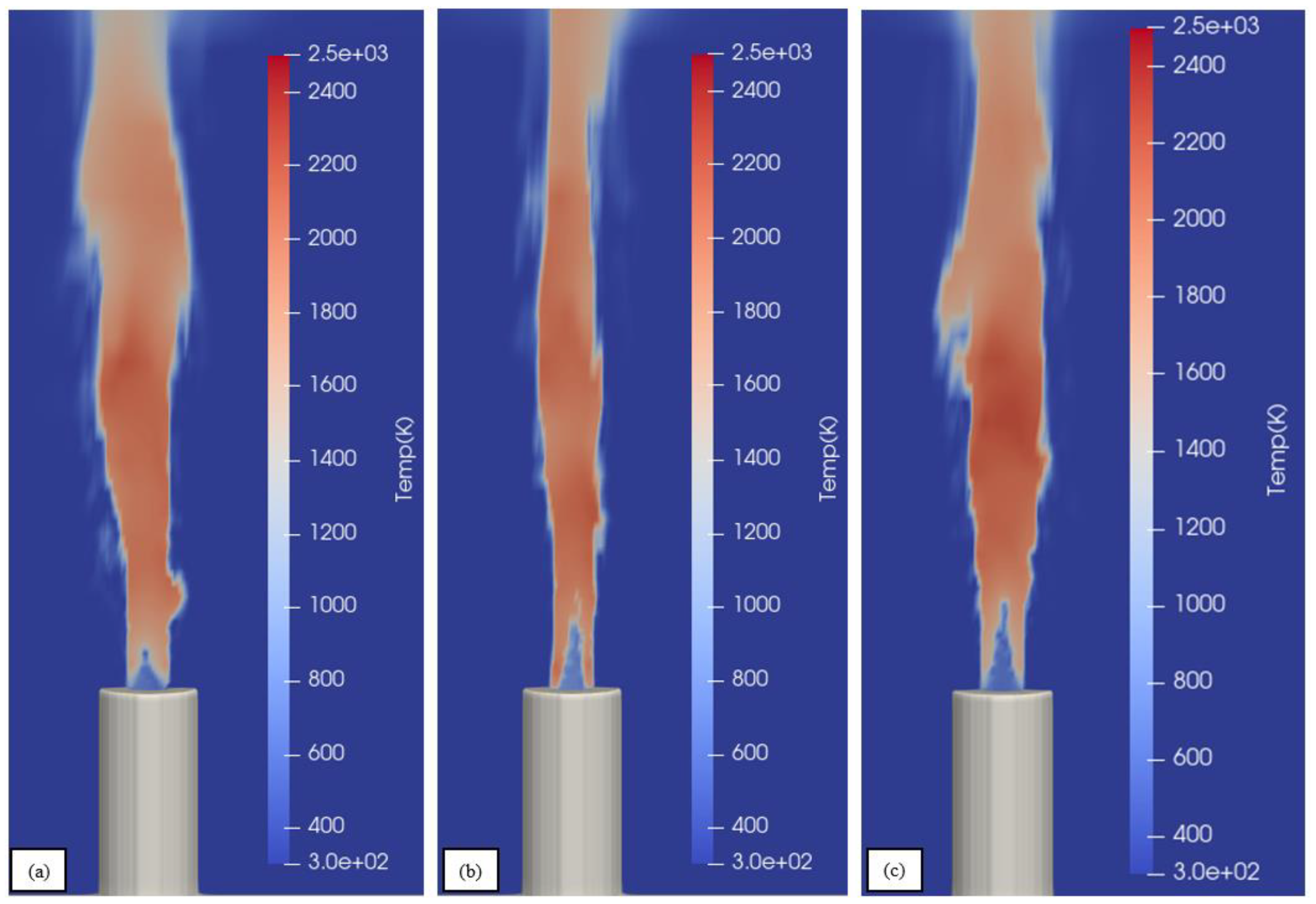
Figure 11.
Utility flare versus air assisted flare operation; (a) 0.42kg/min gas and 0kg/min air, (b) 0.42kg/min gas and 5.7kg/min air, (c) 0.42kg/min gas and 6.6kg/min air, (d) 0.42kg/min gas and 8.2kg/min air.
Figure 11.
Utility flare versus air assisted flare operation; (a) 0.42kg/min gas and 0kg/min air, (b) 0.42kg/min gas and 5.7kg/min air, (c) 0.42kg/min gas and 6.6kg/min air, (d) 0.42kg/min gas and 8.2kg/min air.
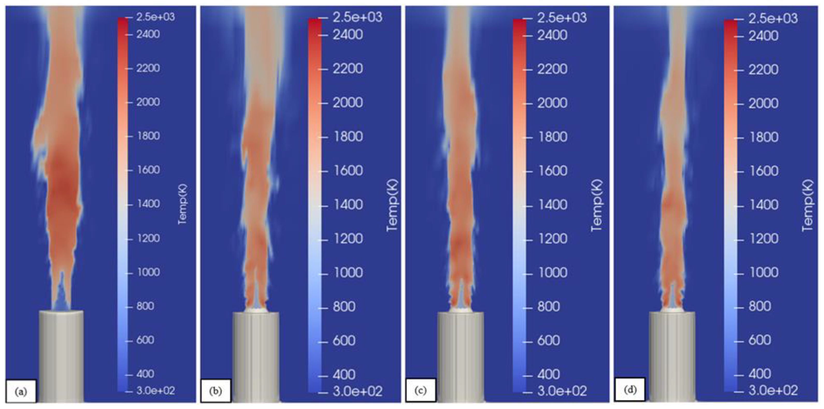
Figure 12.
Data sampling locations: (a) 0.42kg/min gas and 0kg/min air, (b) 0.42kg/min gas and 5.7kg/min air, (c) 0.42kg/min gas and 6.6kg/min air, (d) 0.42kg/min gas and 8.2kg/min air.
Figure 12.
Data sampling locations: (a) 0.42kg/min gas and 0kg/min air, (b) 0.42kg/min gas and 5.7kg/min air, (c) 0.42kg/min gas and 6.6kg/min air, (d) 0.42kg/min gas and 8.2kg/min air.
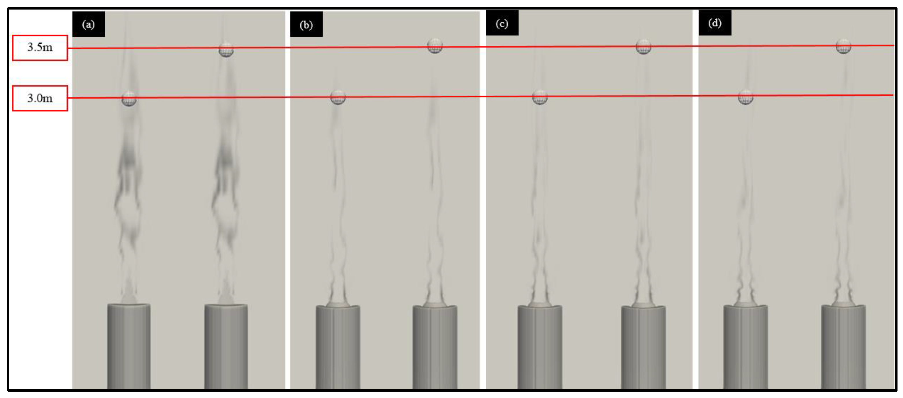
Figure 13.
Utility flare soot formation; (a) 0.3kg/min gas, (b) 0.36kg/min gas, (c) 0.42kg/min gas.
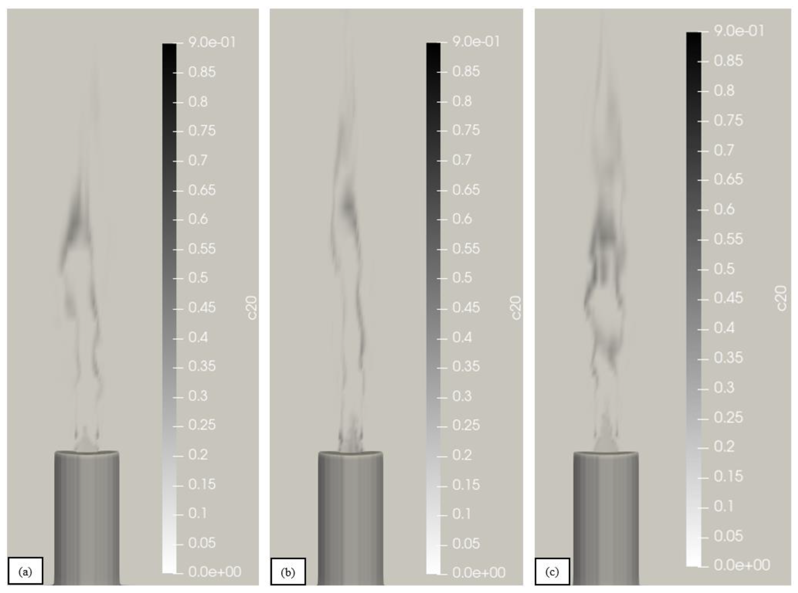
Figure 14.
Utility flare versus air assisted flare soot formation; (a) 0.42kg/min gas and 0kg/min air, (b) 0.42kg/min gas and 5.7kg/min air, (c) 0.42kg/min gas and 6.6kg/min air, (d) 0.42kg/min gas and 8.2kg/min air.
Figure 14.
Utility flare versus air assisted flare soot formation; (a) 0.42kg/min gas and 0kg/min air, (b) 0.42kg/min gas and 5.7kg/min air, (c) 0.42kg/min gas and 6.6kg/min air, (d) 0.42kg/min gas and 8.2kg/min air.
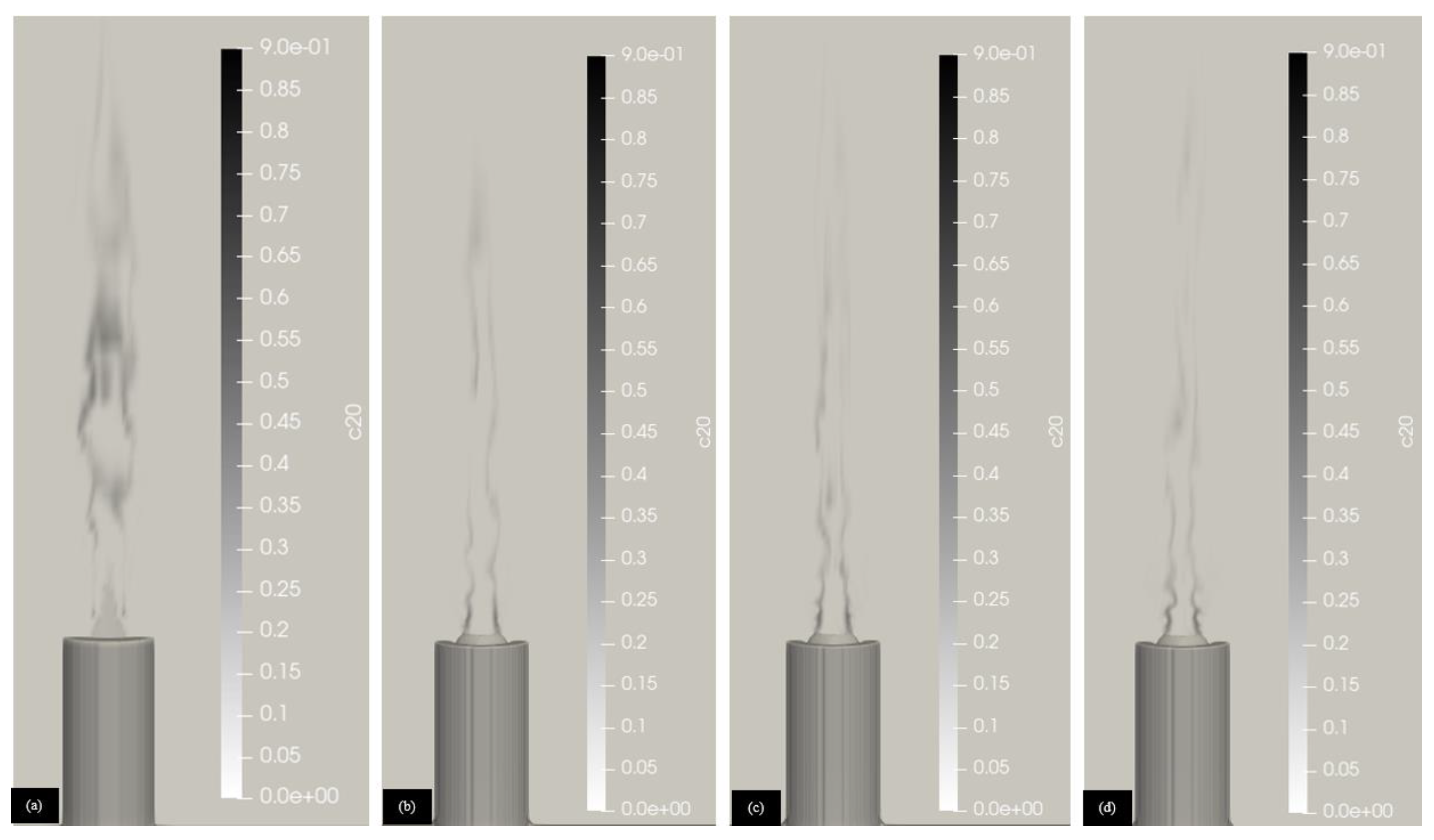
Figure 15.
Soot formation (mass %) of the utility and air assisted cases at sampling location 0m x-axis, 0m y-axis, 3m z- axis.
Figure 15.
Soot formation (mass %) of the utility and air assisted cases at sampling location 0m x-axis, 0m y-axis, 3m z- axis.
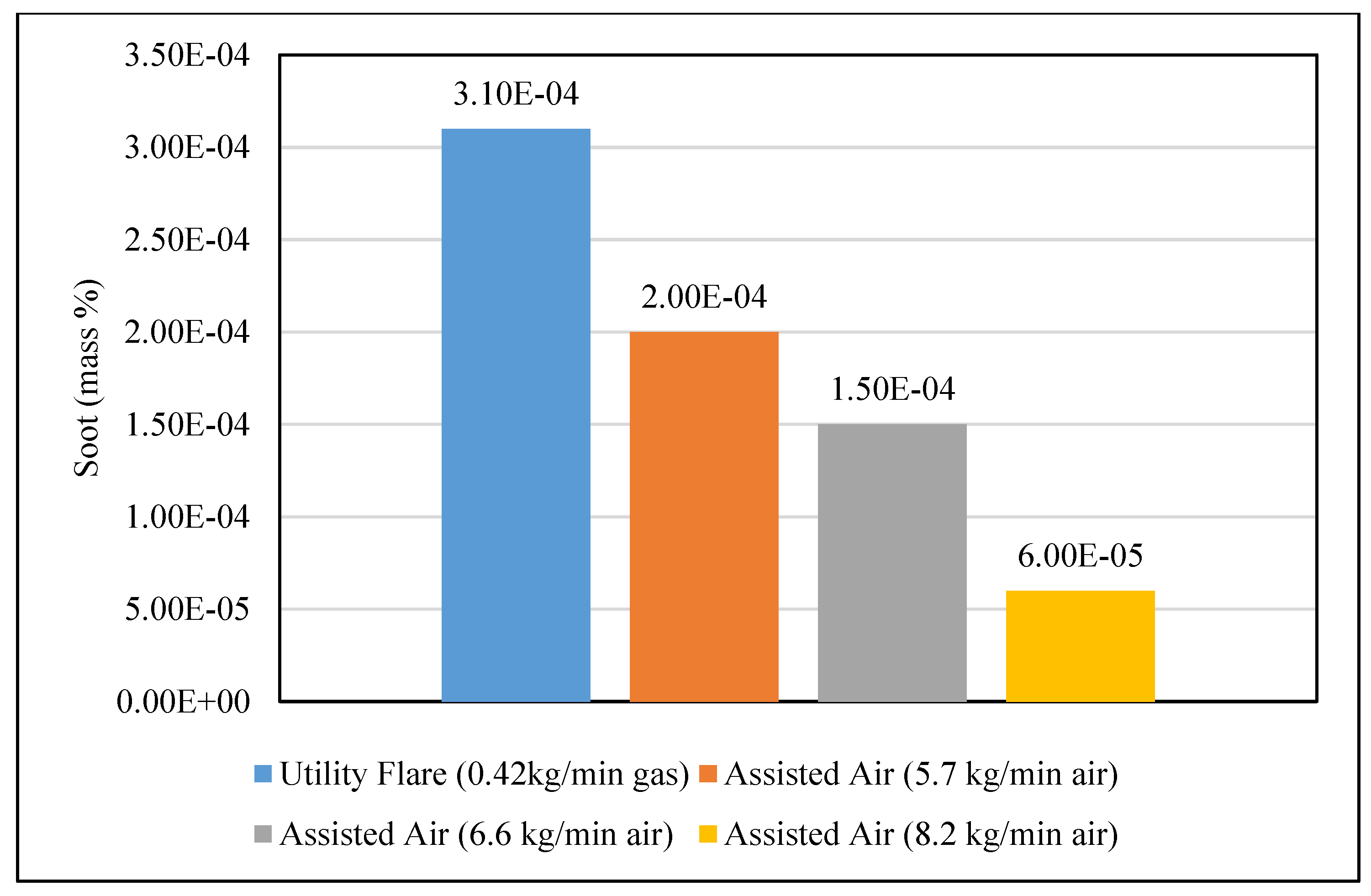
Figure 16.
Soot formation (mass %) of the utility and air assisted cases at sampling location 0m x-axis, 0m y-axis, 3.5m z-axis.
Figure 16.
Soot formation (mass %) of the utility and air assisted cases at sampling location 0m x-axis, 0m y-axis, 3.5m z-axis.
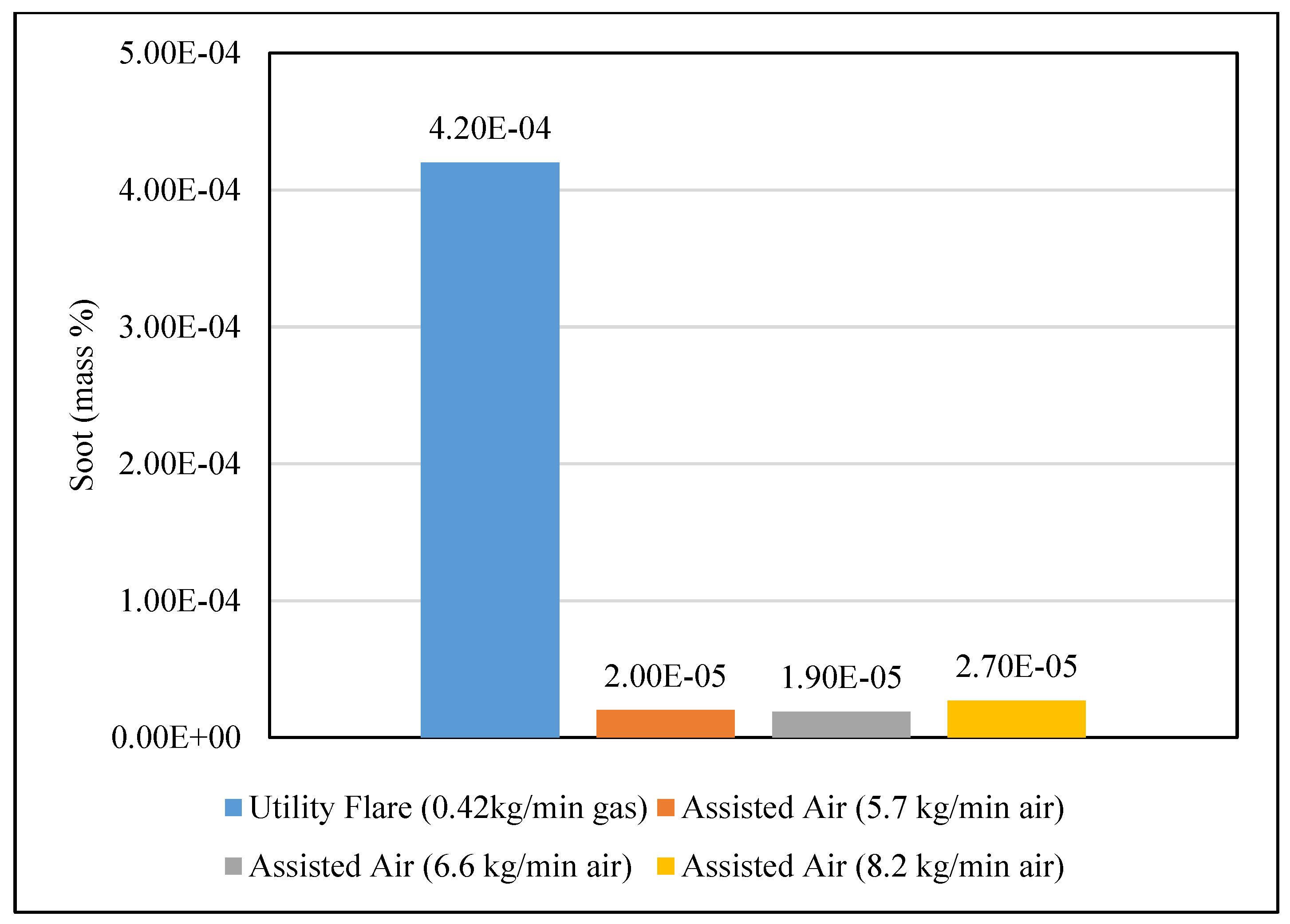
Figure 17.
CE of the utility and air assisted flare at sampling location 0m x-axis, 0m y-axis, 3m z-axis.
Figure 17.
CE of the utility and air assisted flare at sampling location 0m x-axis, 0m y-axis, 3m z-axis.
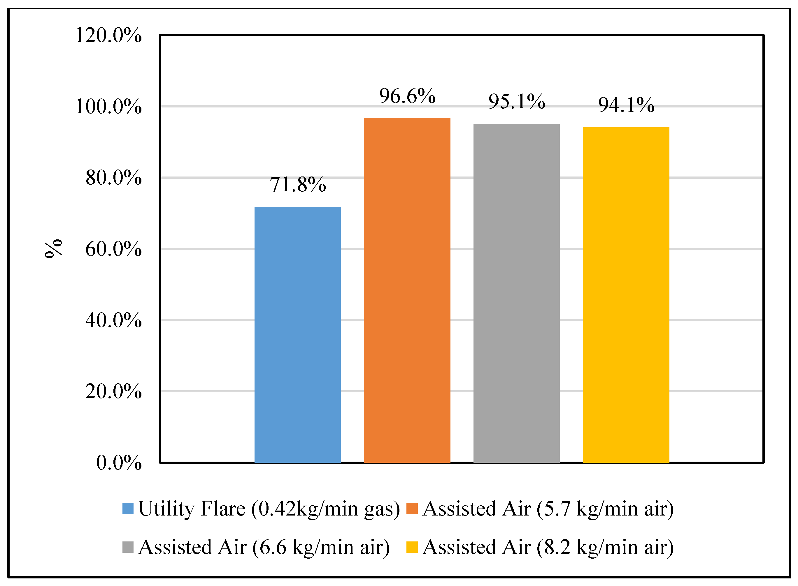
Figure 18.
CE of the utility and air assisted flares at sampling location 0m x-axis, 0m y-axis, 3.5m z-axis.
Figure 18.
CE of the utility and air assisted flares at sampling location 0m x-axis, 0m y-axis, 3.5m z-axis.
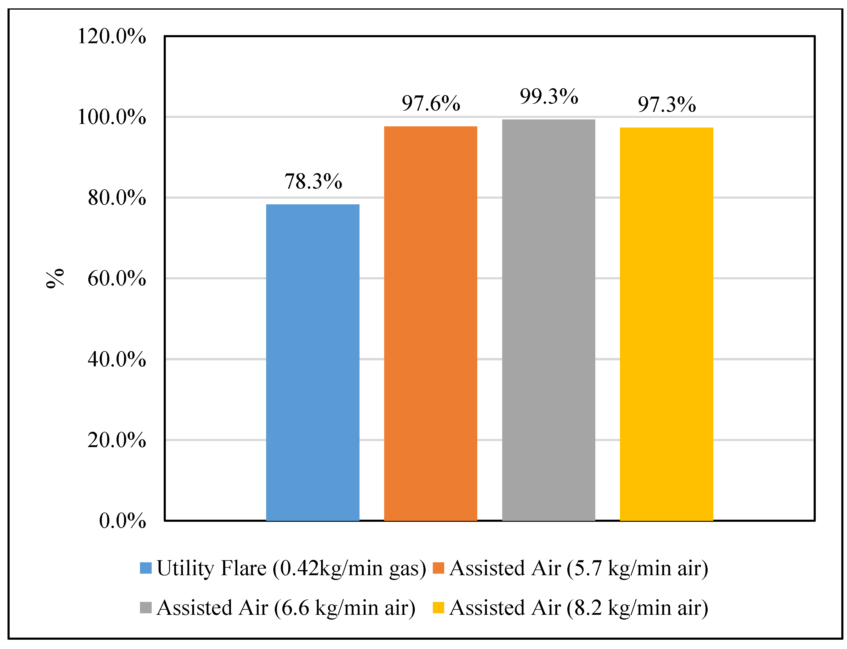
Figure 19.
DRE of the utility and air assisted flare at sampling location 0m x-axis, 0m y-axis, 3m z-axis.
Figure 19.
DRE of the utility and air assisted flare at sampling location 0m x-axis, 0m y-axis, 3m z-axis.
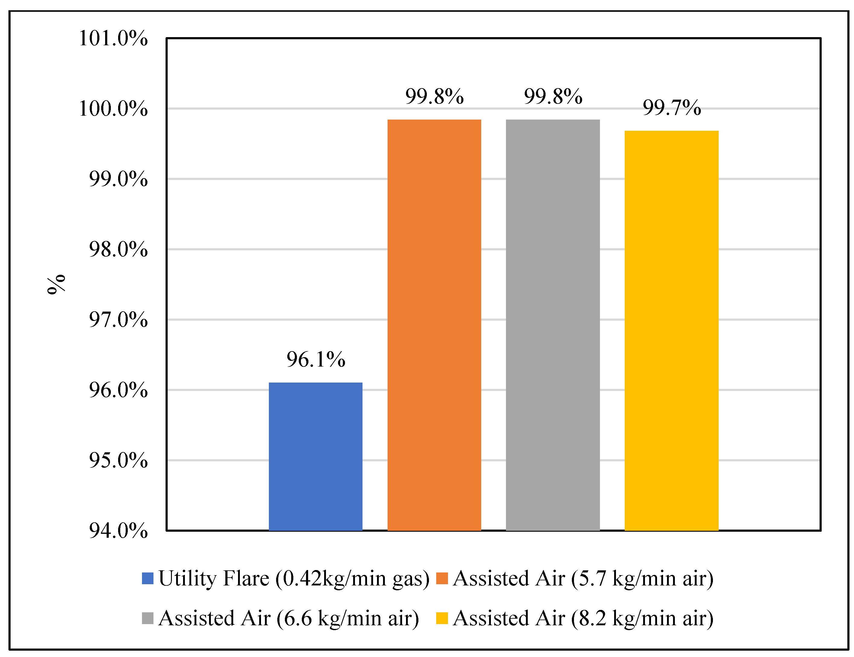
Figure 20.
DRE of the utility and air assisted flare at sampling location 0m x-axis, 0m y-axis, 3.5m z-axis.
Figure 20.
DRE of the utility and air assisted flare at sampling location 0m x-axis, 0m y-axis, 3.5m z-axis.
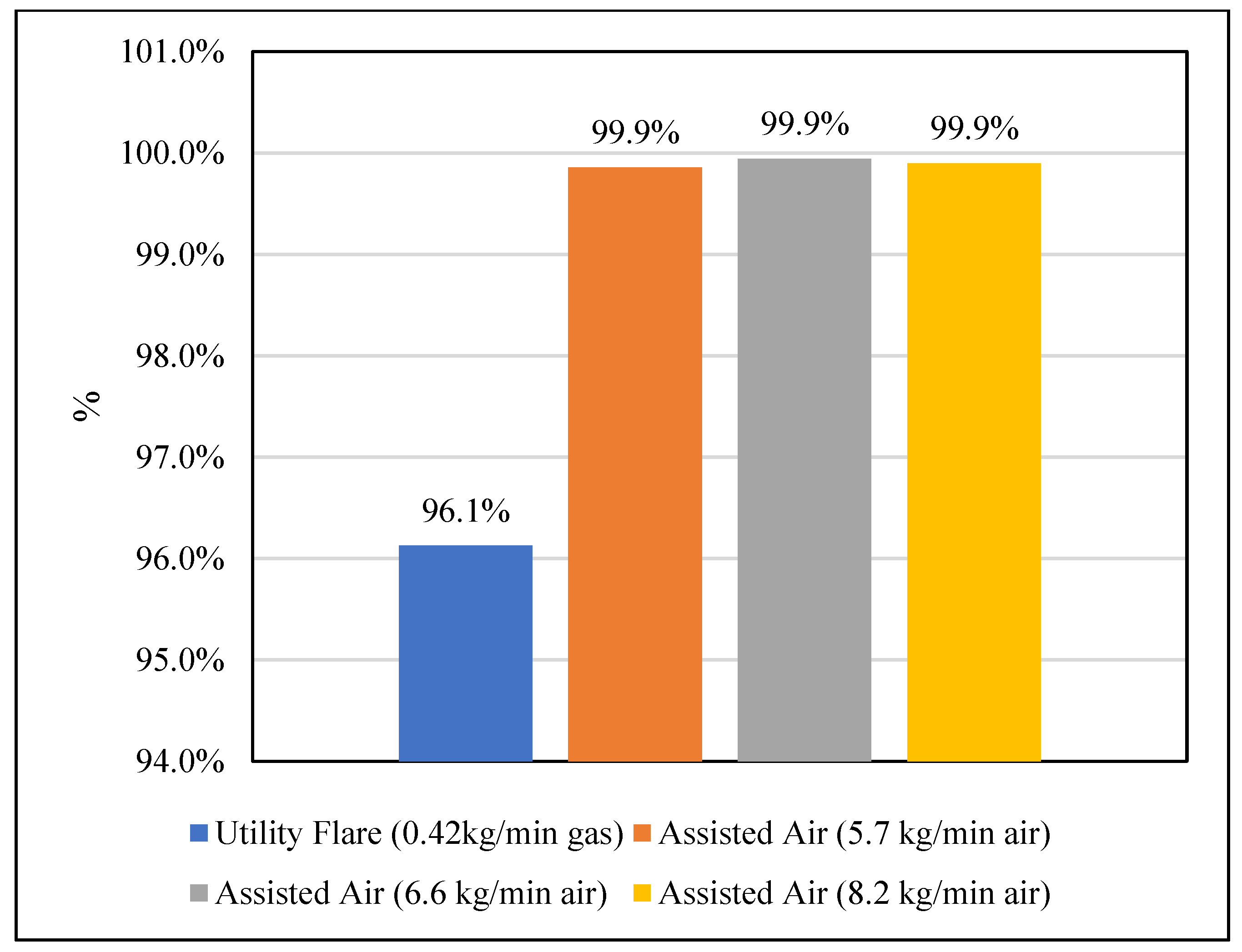
Figure 21.
DRECH4 of the utility and air assisted flare at sampling location 0m x-axis, 0m y-axis, 3m z-axis.
Figure 21.
DRECH4 of the utility and air assisted flare at sampling location 0m x-axis, 0m y-axis, 3m z-axis.
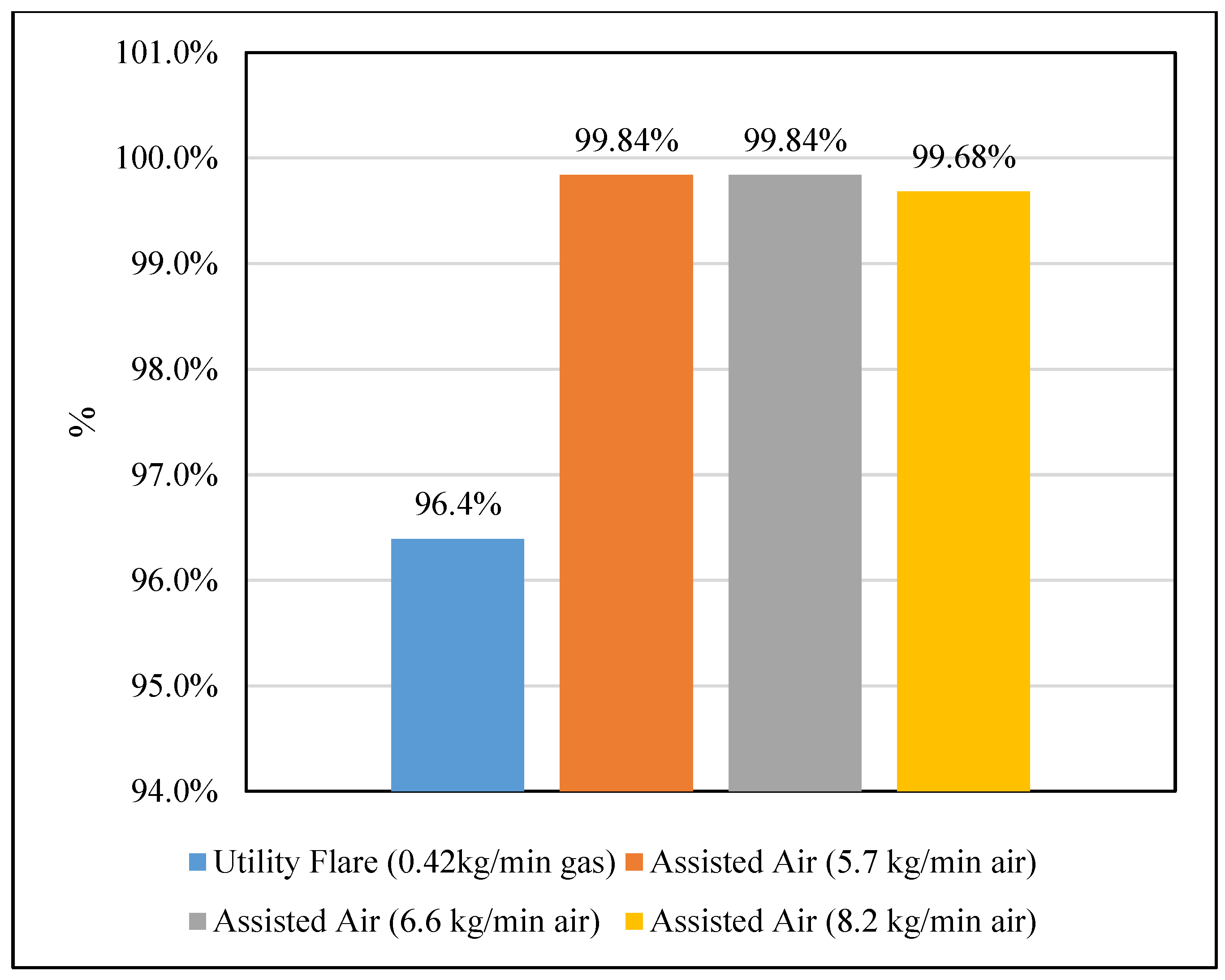
Figure 22.
DRECH4 of the Utility and air assisted flare at sampling location 0m x-axis, 0m y-axis, 3.5m z-axis.
Figure 22.
DRECH4 of the Utility and air assisted flare at sampling location 0m x-axis, 0m y-axis, 3.5m z-axis.
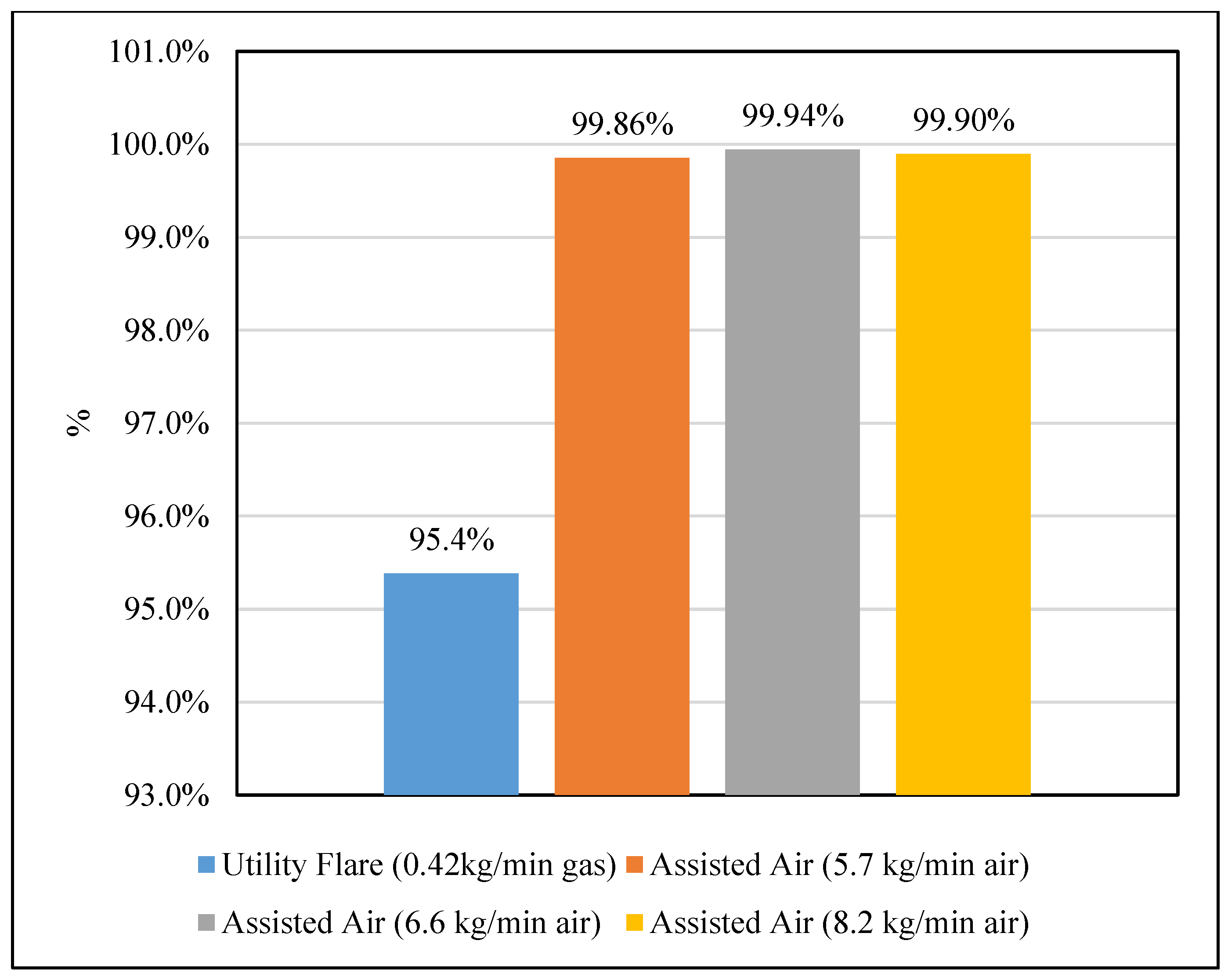

Table 1.
Case study gas composition.
| Basis = 100 kgmole/h | |||||
|---|---|---|---|---|---|
| Components | Mole (%) | Kg mole | MWt | Kg | Mass (%) |
| C1 | 83.34 | 83.34 | 16 | 1333.44 | 0.693 |
| C2 | 9.501 | 9.501 | 30 | 285.03 | 0.148 |
| C3 | 3.391 | 3.391 | 44 | 149.204 | 0.078 |
| C6+ | 0.232 | 0.232 | 86 | 19.952 | 0.010 |
| CO2 | 1.713 | 1.713 | 44 | 75.372 | 0.039 |
| H2S | 1.816 | 1.816 | 34 | 61.744 | 0.032 |
| N2 | 0.007 | 0.007 | 28 | 0.196 | 0.000 |
| Total | 100 | 100.00 | 1925 | 1 | |
Table 2.
Utility flare cases average temp, CO, CO2 and soot at both sampling locations.
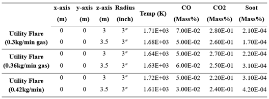 |
Table 3.
Utility flare cases average C1, C2, C3 and C6+ at both sampling locations.
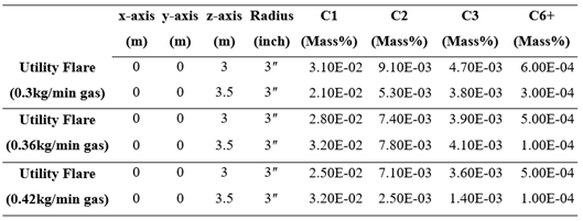 |
Table 4.
Utility and air assisted flare average temp, CO, CO2 and soot at both sampling locations.
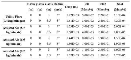 |
Table 5.
Utility and air assisted flare average C1, C2, C3 and C6+ at both sampling locations.
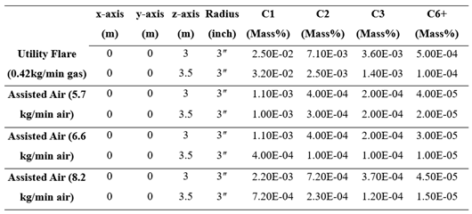 |
Table 6.
Combustion Efficiency (CE) & Destruction and Removal Efficiency (DRE) of the utility flare cases.
Table 6.
Combustion Efficiency (CE) & Destruction and Removal Efficiency (DRE) of the utility flare cases.
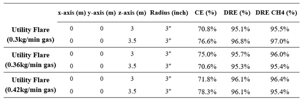 |
Table 7.
Combustion Efficiency (CE) & Destruction and Removal Efficiency (DRE) of the utility and air assisted flares.
Table 7.
Combustion Efficiency (CE) & Destruction and Removal Efficiency (DRE) of the utility and air assisted flares.
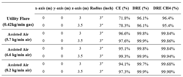 |
Table 8.
Soot formation and CE of the utility and air assisted flares.
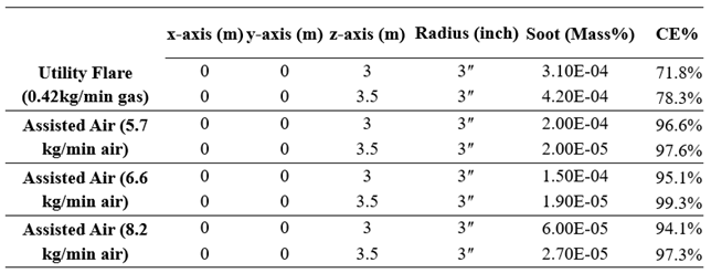 |
Table 9.
Fuel carbon balance for the utility and air assisted flares.
 |
Disclaimer/Publisher’s Note: The statements, opinions and data contained in all publications are solely those of the individual author(s) and contributor(s) and not of MDPI and/or the editor(s). MDPI and/or the editor(s) disclaim responsibility for any injury to people or property resulting from any ideas, methods, instructions or products referred to in the content. |
© 2024 by the authors. Licensee MDPI, Basel, Switzerland. This article is an open access article distributed under the terms and conditions of the Creative Commons Attribution (CC BY) license (http://creativecommons.org/licenses/by/4.0/).
Copyright: This open access article is published under a Creative Commons CC BY 4.0 license, which permit the free download, distribution, and reuse, provided that the author and preprint are cited in any reuse.


