1. Introduction
Low Power Wide Area Network (LPWAN) [
1] has now emerged as one of the most popular wireless networks for the Internet of Things (IoT). LPWAN has found various applications such as smart city, smart logistics, and smart farming. Long Range Wide Area Network (LoRaWAN) [
2] is one of the LPWAN technologies that has received much attention for the past several years due to its low power consumption, large coverage area, high security, long battery life, and low cost. Compared with proprietary LPWAN technologies such as NB-IoT [
3] and Sigfox [
4], the non-proprietary LoRaWAN opens for individual users to adopt, build, learn, and research on the technology freely.
LoRaWAN uses the chirp spread spectrum (CSS) as a signal modulation technique in the physical layer. The packet and propagation characteristics are classified into groups of spreading factors (SFs) that are determined based on the received signal strength indicator (RSSI) and propagation distance of each packet. The typical values of SF are 7-12. The smaller SF offers higher data rate and shorter time-on-air (ToA) while the larger SF offers lower data rate and longer ToA. Since LoRaWAN adopts the pure ALOHA protocol, which allows simultaneous packet transmission by multiple end devices or nodes over a common radio channel; therefore, it inevitably suffers from packet loss due to collision. Note that, a packet collision is confirmed when two or more colliding packets have the same SF value and frequency, or same chirp rate. To alleviate the problem, altering data rate and thus ToA of end devices or SF allocation, is a widely used approach.
Various pieces of research focused on the applications of LoRaWAN. Examples include deploying gas sensors to remotely collect data for air pollution control [
5] and the integration of LoRaWaN to the smart water resource management equipped with measurement systems of water availability, soil moisture, topography, and plant identification [
6,
7]. They found that LoRaWAN could improve the data transmission and thus the data extraction rate (DER), which is the ratio between the success sending data packet and all data packets in a defined period.
Other previous research explored and improved LoRaWAN performance in different environments. The LoRaWAN network infrastructure was implemented for a universal sensor, and proved to consume lower energy and operated well under real-life conditions [
8]. The LoRaWAN performance with mobile nodes was evaluated in an urban environment and was found to provide shorter data transmission range than the open environments [
9]. The path-loss propagation model for LoRaWAN was then optimized in some certain environment to ensure the positive results [
10].
A default mechanism used for optimizing data rate, ToA, and energy consumption of an end device in LoRaWAN is the adaptive data rate (ADR) [
11]. The ADR optimizes these parameters by considering RSSI and link budget. When multiple nodes are placed in a confined area, their RSSI values are nearly the same, so do their SF values. Although the ADR is activated, the SF vallues are not sufficiently distributed, thus the packet collisions still occur. Therefore, several previous works aimed on improving the network performance, reducing packet collision by better SF allocation or assignment.
Basically, there are six techniques for improving SF assignments, which were summarized in [
2]. The techniques include SNR-based, mathematical model, RSSI-based, ToA, distance-based, and AI and machine learning techniques.
The SNR-based SF technique focuses on optimizing the gain and transmit power to reduce the transmission failure associated by noise and interference. In [
12] equal-interval-based (EIB) and equal-area-based (EAB) SF allocation methods were proposed. Both methods compared SNR values with SNR thresholds based on the gateway specification. In [
13], the SNR optimization algorithm was proposed to improve the packet delivery ratio (PDR) and energy efficiency over the original ADR.
The RSSI-based and ToA techniques were designed to mitigate SF collisions during message transmission. Specifically, they aimed to prevent multiple devices from transmitting messages using the same SF values and radio channels simultaneously, thereby enhancing overall network efficiency and reliability. For instance, the EXPLoRa-SF algorithm compared the RSSI values with the sensitivity levels and divided them into six groups with equal number of nodes [
14]. Then, the EXPLoRa-AT algorithm proposed to use the “sequential waterfilling” to select the optimal SF values for certain ToAs for proper selection of radio channel for message transmission [
15].
The distance-based technique involves calculating the optimal transmit power allocation by considering both distance and assigned SF value [
16]. The concept of this technique in fact, aligns closely with SNR-based SF allocation, which focuses on adjusting the transmit power to resist noise and interference.
In [
17] and [
18], mathematical models combined with machine learning approaches were reported. In [
18], the reinforcement learning (RL)-based method for SF channel allocation in one-hop and in the LoRa mesh network was proposed. The equation for properly selecting the new SF value based on environmental conditions was then developed. The RL method optimized the SF value by providing positive rewards if the SF effectively reduces collision rates and negative rewards otherwise. Consequently, the optimal SF value that minimizes data collision rates was determined. In addition, [
18] proposed an algorithm that incorporates node distance information, then utilized the supervised machine learning for transmit power allocation and employed the RL method for SF allocation.
Apart from the abovementioned techniques, the statistical approach has become another promising approach to improve SF assignment. In [
19], the researchers proposed the Quantile Classification of Variance from the Mean (QCVM) method that uses the statistical method namely, the quantile classification to group RSSI data considering their average and probability density function (PDF). Then, they proposed the Standard Deviation (SD) classification method that analyzed RSSI data of nodes before separating them by the standard deviation (SD) and re-assigning the SF values [
20].
It was known that most SF allocation algorithm developments began with simulations prior to the actual implementations. The node locations were commonly generated in the uniform random distribution, which is the default setting in most LoRaWAN simulators. However, the real-life node patterns often exhibit non-uniform or biased node distributions; thus, the uniform random distribution does not always give accurate insights in real-world scenarios, and potentially compromising the efficacy of prior algorithms in such contexts.
This research introduces the Geometric Distribution (GD) algorithm, a novel approach that leverages the Probability Mass Function (PMF) of the geometric distribution mathematical model [
21] to address the challenge of non-uniform or biased SF node distribution. By incorporating this framework, the GD algorithm aims to enhance the default Adaptive Data Rate (ADR) mechanism in the LoRaWAN. The key of the GD algorithm is to identify the optimal distribution format for the intensive SF values by assigning weights to each SF category. The algorithm seeks to determine the weight factors (
w) that best capture the number of occurrences for each SF. These weight factors (
w) are intricately linked to the geometric distribution factor (
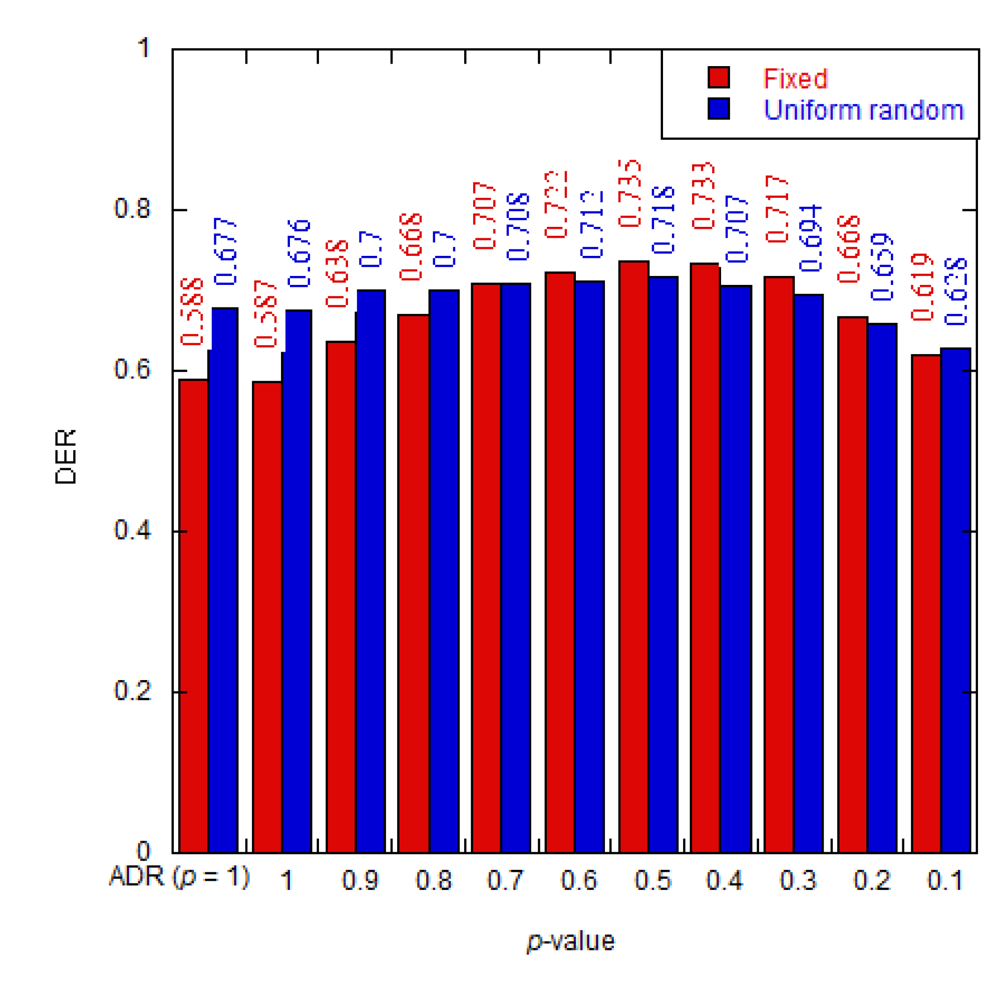
p-value) for which we aimed to identify the optimal value and corresponding weight factors (
w) that yield the highest DER.
Our research applied the proposed GD algorithm to the LoRaWAN simulations conducted using the LoRaSIM simulator. To assess the impact of node distribution on network performance, a comparative analysis was undertaken. This analysis compared results obtained from the uniform random node distribution scenario to those obtained from the fixed node distribution assumed based on locations of dairy farms around the Photharam district, Ratchaburi province, Thailand [
22]. This particular site was selected because it plans to implement Internet of Things (IoT) sensors to collect behavior data from dairy cows. The novelty of our algorithm lies in its ability to work effectively with biased node distributions and still achieve high DER values. This adaptability ensures the algorithm’s efficacy across various scenarios, providing valuable insights for improving network performance under diverse conditions.
The paper is divided into subsections as follows.
Section 2 provides a brief overview of LoRaWAN.
Section 3 delves into the comparison of fixed and random node simulation, while
Section 4 and
Section 5 expound on the geometric distribution mathematical model and the proposed algorithm, respectively.
Section 6 covers the details of the experiment simulation, and the discussion and analysis of results are presented in
Section 7. The research concludes with a summarizing section outlining the key findings and implications of the study.
2. LoRaWAN Overview
LoRa is a protocol in the physical layer of an IoT network. This protocol operates in the industrial, scientific, and medical radio band (ISM band) or 902 – 928 MHz in Thailand. LoRa protocol can endure the noise floor and interference by Chirp Spread Spectrum (
CSS) techniques. The highlighted advantages are low power consumption and long-range coverage area. The characteristics of the CSS modulation depend on the LoRa’s parameters such as bandwidth (
BW), SF, Coding Rate (
CR), and the airtime defined in terms of the Symbol time (TS) shown in equation (1). The bit rate (
Rb) is related to
BW, SF, and
CR as shown in equation (2).
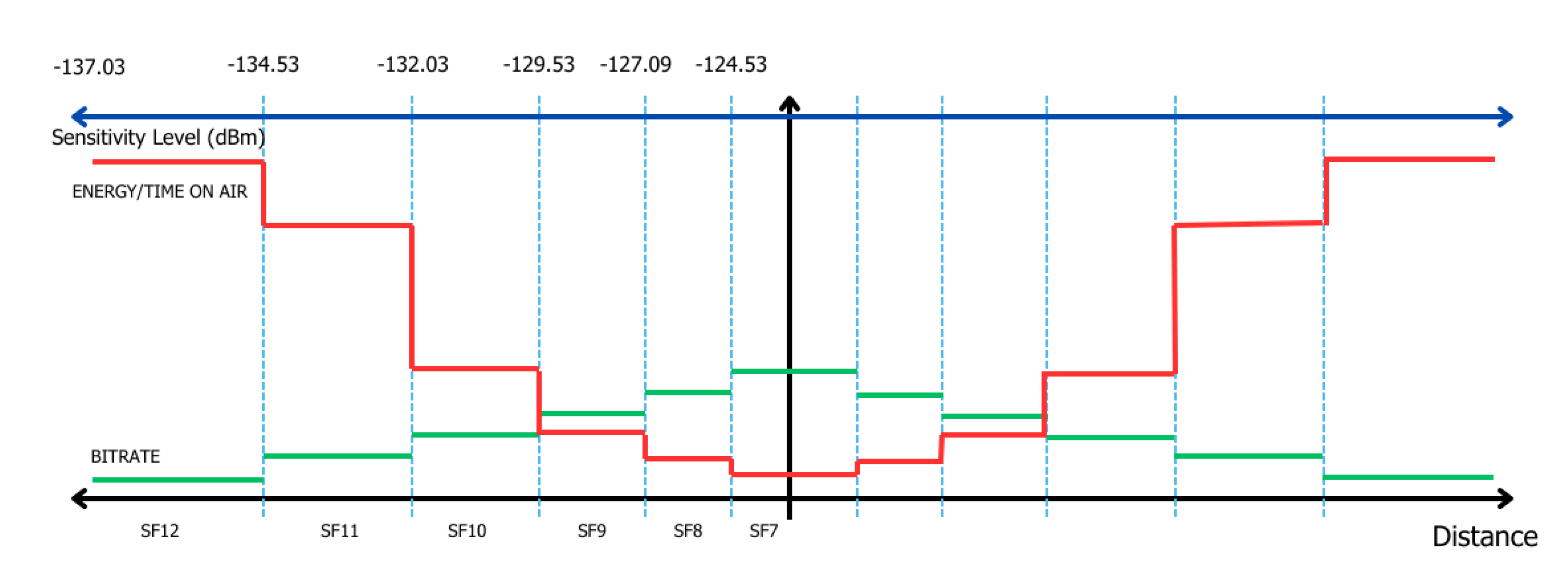
LoRaWAN is a network architecture consisting of end devices or nodes that employ the LoRa protocol for transmitting and receiving packets, LoRa gateway, network server, and application server. In LoRaWAN, we can define the data rate, airtime, and signal range by assigning the SF values, which is the unique parameter in the LoRa modulation, as shown in
Figure 1.
LoRaWAN utilizes the Adaptive Data Rate (ADR), which is a default mechanism for optimizing the data rate, airtime, distance, and energy consumption, when the signal strength varies dynamically such as in the case of dense and moving nodes. The link budget is the RSSI sensitivity level, which depends on the Signal-to-Noise Ratio (
SNR), Noise Figure of receiver (
NF), and BW. The link budget is presented in terms of the sensitivity value (
S) shown in equation (3). The SNR limit is dependent on the end device, and the
NF of a typical LoRa gateway chipset is 7 dB [
11]. The sensitivity level is also displayed in
Figure 1.
3. Network Simulations for Fixed and Uniform Uniform Random Patterns of Nodes
The network simulation is the important approach to better anticipate the results of the actual network performance. It also shed some lights on what the network performance would be like in case the actual implementation cannot take place. However, most previous simulation works relied on generating a uniform random node pattern that could significantly deviate from the real-world scenario. This section aims on understanding the effect of node patterns on SF assignment and network performance by comparing fixed and random node patterns using the default ADR scheme.
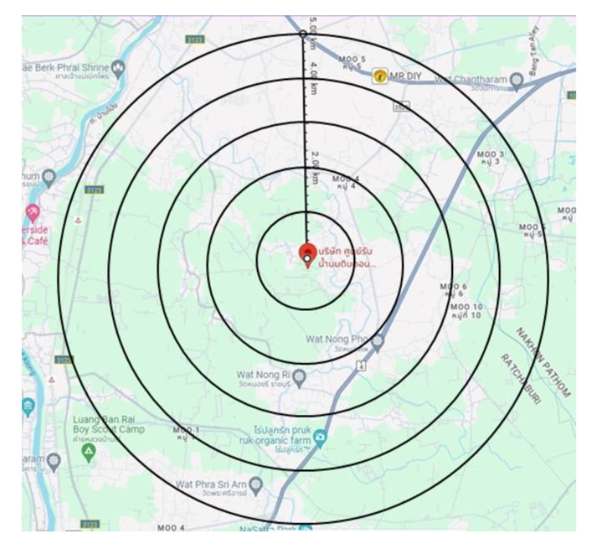
Before constructing the node pattern, the propagation path loss model suitable for the study area was selected for the simulation. In our investigation, we conducted a survey at a considerable number of dairy farms in the Photharam district of Ratchaburi, Thailand. This area has a potential to adopt smart livestock technologies, and some farms had already pursued that. We installed the LoRa gateway at Centermilk Farm and then conducted several drive tests in 5 km radius as shown in
Figure 2 to measure the LoRa signal strength before creating a map to locate dairy farms within the test area. Photharam district is situated outside urban areas, characterized by small buildings and villages. While present, these structures are not as numerous or densely populated as in urban. This environment thus aligns better with the suburban Hata-Okumura path loss model [
23] as indicated by equations (4)-(8).
where
Lc is the power of path loss,
d is the distance of end devices in meter,
hm is the height of end devices in meter,
f is the frequency in Kilohertz
hb is the height of the gateway in meter.
Figure 2.
Location of dairy farms at Photharam district, Ratchaburi, Thailand.
Figure 2.
Location of dairy farms at Photharam district, Ratchaburi, Thailand.
In our research, we assigned 1,500 nodes to represent 1,500 connected dairy cows raised on the dairy farms in Photharam district, Ratchaburi. Note that, the connected dairy cows are those tagged with the IoT sensors. We introduced node positions in the 2D plane with
x and
y coordinates, as expressed in equations (9) and (10). Subsequently, we calculated the distance
D from the node to a gateway using the Pythagorean formula as shown in equation (11).
where
Dmax is the coverage area in meter,
x and y are the positions in the 2-dimensional plane,
D is the distance between the node and the gateway in meter,
A, B, and C are the values between 0 to 1.
First, we utilized the LoRaSim simulator to randomize
A,
B, and
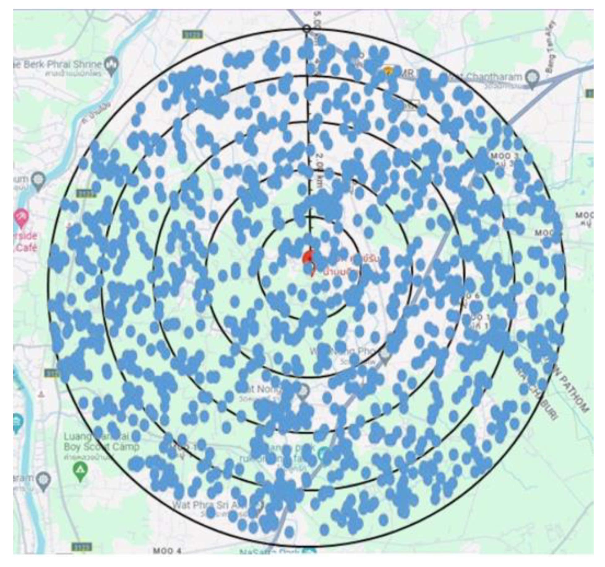
C constants to generate the uniform random node pattern as shown in
Figure 3. Then, we assigned certain values of
A, B, and
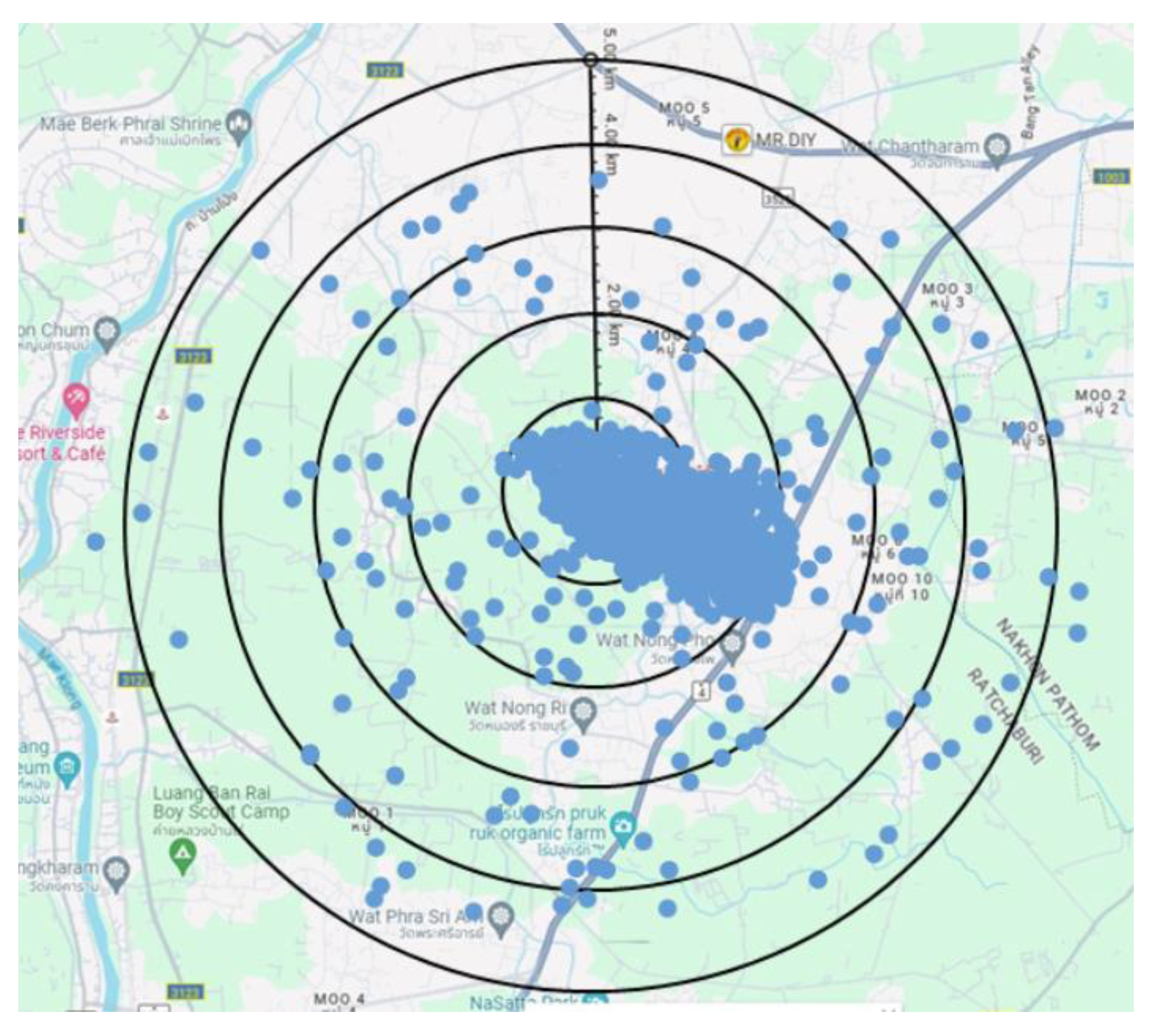
C constants using Equations (9)-(11) to reflect the actual locations of dairy farms, and consequently, the connected cows raised on those farms. The actual or fixed pattern shown in
Figure 4 clearly exhibits a biased node distribution where most nodes are confined within 2 km radius from the center.
After the node pattern was constructed, the node’s SF values of both patterns were assigned using the default ADR mechanism in LoRaSim. The proportion of SF assignment was observed and measured and the DER values were computed. The results are shown in the
Table 1. At distances 2 and 3 km for both uniform random and fixed patterns, every node is assigned as SF7. The DER values are nearly identical at around 51%. At 4 and 5 km, more nodes are distributed to SF8 and SF9 respectively, but the majority is still SF7. For the fixed node pattern, above 89% of nodes are SF7, while the number is clearly lower for the uniform random pattern. This disparity in SF assignment directly affects DER values, with the uniform random pattern exhibiting 6.2% and 8.7% higher than those of the fixed pattern at 4 and 5 km, respectively. The results somewhat indicate insufficiency of the default ADR scheme in handling actual node distributions.
5. The Geometric Distribution Algorithm for SF Assignment
Reverting to the DER results run by the default ADR scheme, a significant challenge arose since more than 70% of all nodes from the uniform random and fixed patterns were assigned SF7 at 4 and 5 km. To significantly improve the DER, we needed to find the optimal SF distribution by redistributing the number of SF7 nodes using the PMF and determined the weight factor for each SF. Initially, we employed a weight factor (
w), as defined in equations (13)
where
NSF max is the total number of majority SF nodes
wn is the weight factor of new SF7 (
n = 1) to new SF12 (
n = 6) and is defined as
where
n = 1-6
From (12), the summation of
w1 to
w6 must be 1, that is
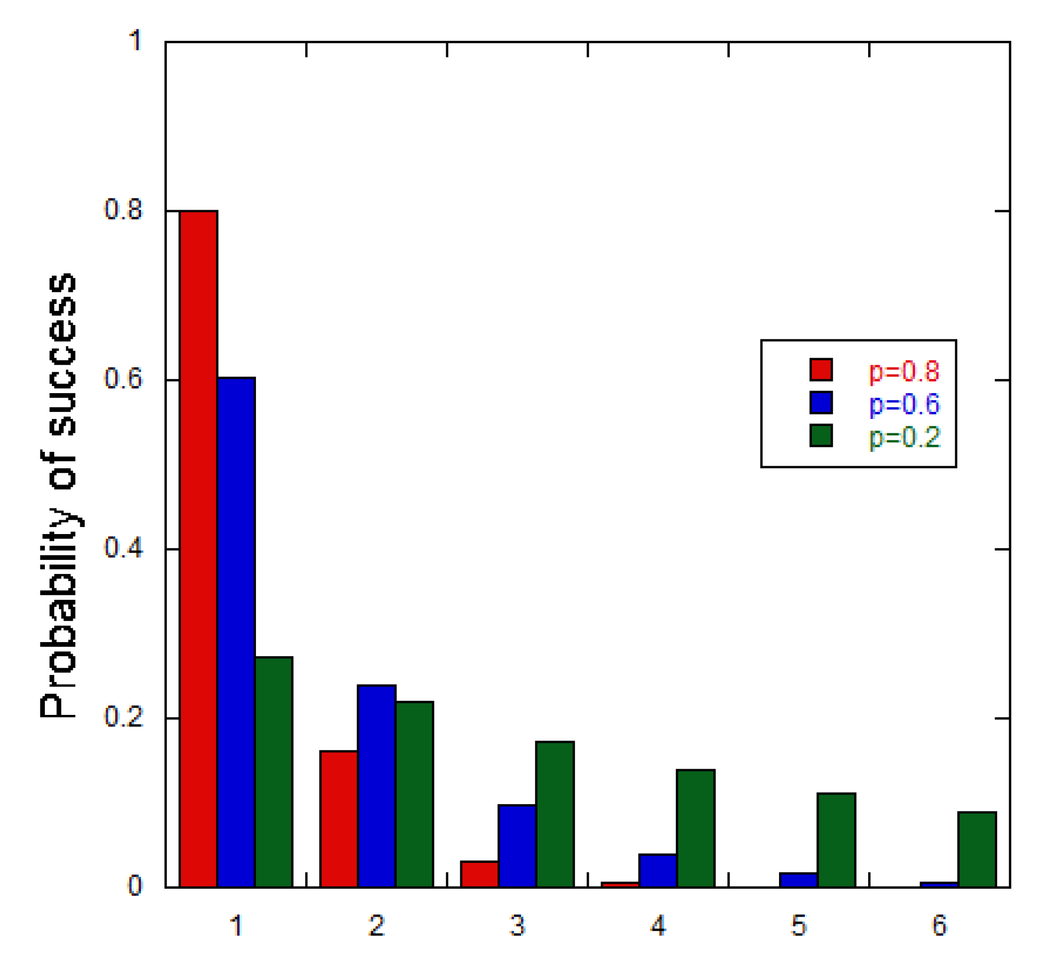
By using this approach, the weight factor always decreases when p in equation (14) increases. The summation of the new weight factors must be 1, as shown in (15). The numbers of new SF7-SF12 respectively, are obtained by multiplying w1 – w6 by NSF max, respectively.
The GD algorithm was then developed and is shown in Algorithm I. First, we input the highest number of nodes with similar SF, which in our case is the SF7, to the proposed GD algorithm. Then, SF7 nodes were separated using the GD approach. The process entered a loop starting at
p = 1 and the corresponding weight factors
w[
x] were multiplied by the SF7 count (N
SF max) to obtain the number of new SFs. The loop iterated as the
p-value decreased by 0.1 decrement. The weight factors were recalculated at each
p-value and thus, the number of new SFs was obtained. The loop continued until the
p-value reached 0.1, marking the end of the algorithm. The resulting set of weight factors at the
p-value equal 1 to 0.1 is presented in
Table 2.
|
Algorithm I: Geometric distribution
|
1:
2:
3:
4:
5:
6:
7:
8:
9:
10:
11:
12:
13:
|
Input: Number of highest SF (NSF max)
Define: Weight factor (w)
Geometric distribution factor (p)
Initialize: p = 1
Do
// Calculate the weight factor of each SF
w[x] ← p * (1 - p) ^ (x - 1) let x = 1, 2, 3, 4, 5, 6
// Calculate the number of each SF
SF[y] ← NSF max* w[x] let x = 1, 2, 3, 4, 5, 6 and y = 7, 8, 9, 10, 11, 12
// Return the new number of each SF
Return SF[7], SF[8], SF[9], SF[10], SF[11], SF[12]
p ← p – 0.1
While p > 0.1 // p starts at 1 to 0.1, with 0.1 decrement
|
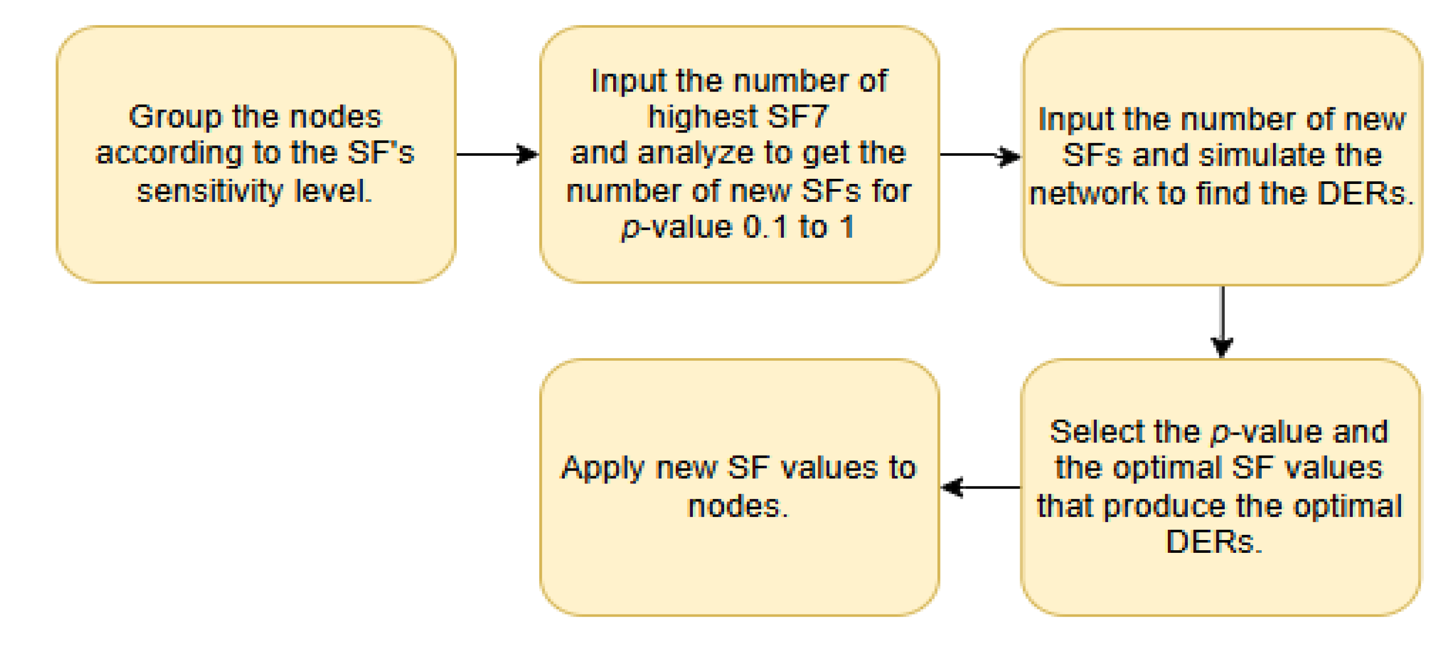
The complete implementation workflow is shown in
Figure 6. Initially, nodes were classified according to sensitivity levels outlined in
Figure 1. After applying the GD algorithm, the sets of weight-classified SF nodes were input to the simulation to determine Data Extraction Rate (DER) values for probabilities ranging from
p = 1 to 0.1. The
p-value that produced the optimal SF and DER values was selected, and finally, the optimized SF values were applied to the nodes.
8. Conclusions
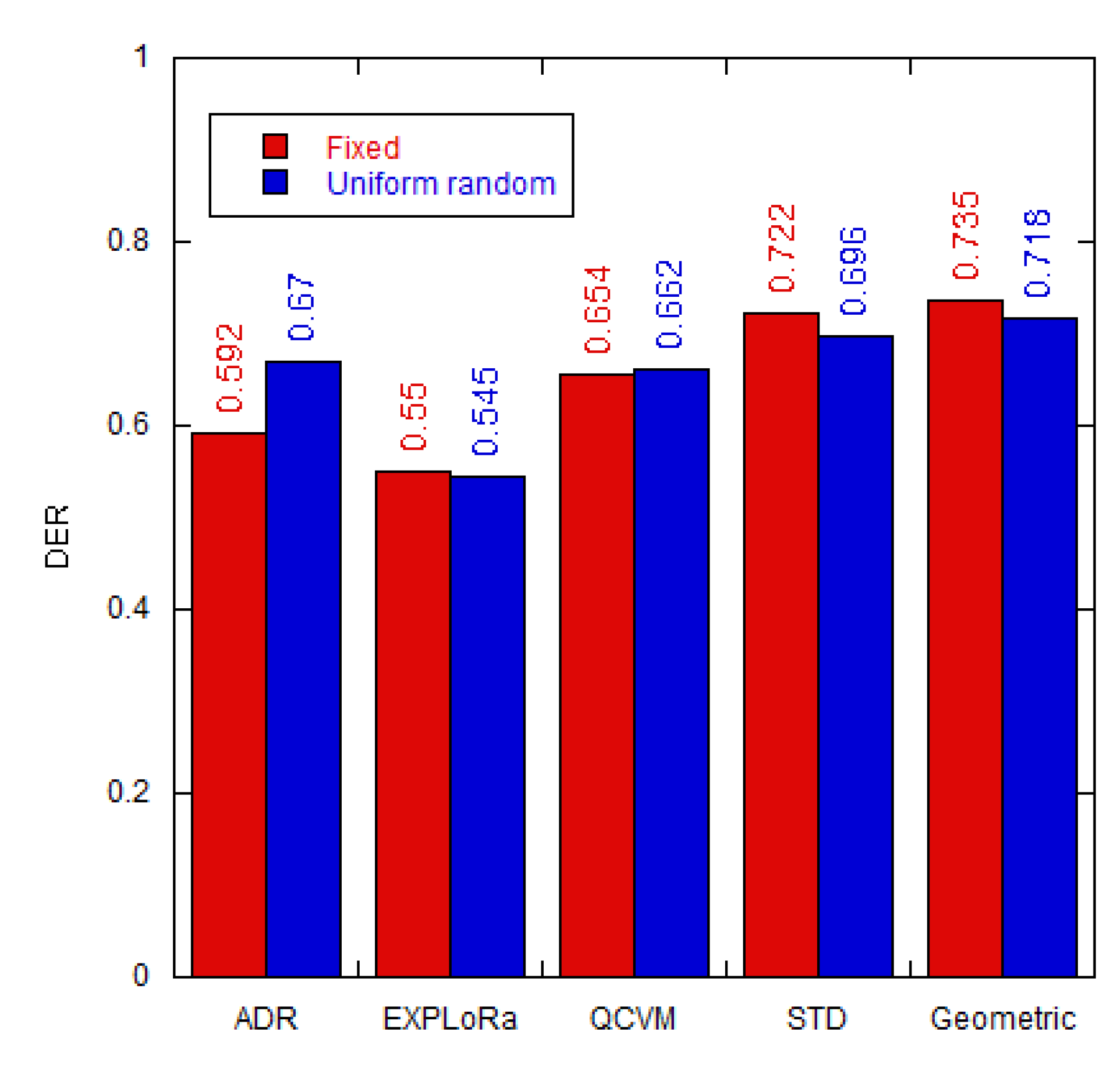
This research endeavored to enhance the performance of the LoRaWAN by addressing collision probability issues, specifically aiming to reduce instances of the same SF. Various algorithms employed in the past often incorporated RSSI optimization on random and normally distributed node patterns. Our contribution to this domain introduced a novel algorithm based on the geometric distribution (GD), where we applied this algorithm to real-world scenarios that possessed certain node patterns. Results from our study indicated that the proposed algorithm achieved significant improvements in both optimal SF assignment and DER values compared to previous algorithms. Specifically, the fixed pattern exhibited an impressive enhancement of 14.3%, while the uniform random pattern exhibited 4.8% enhancement over the default ADR scheme.
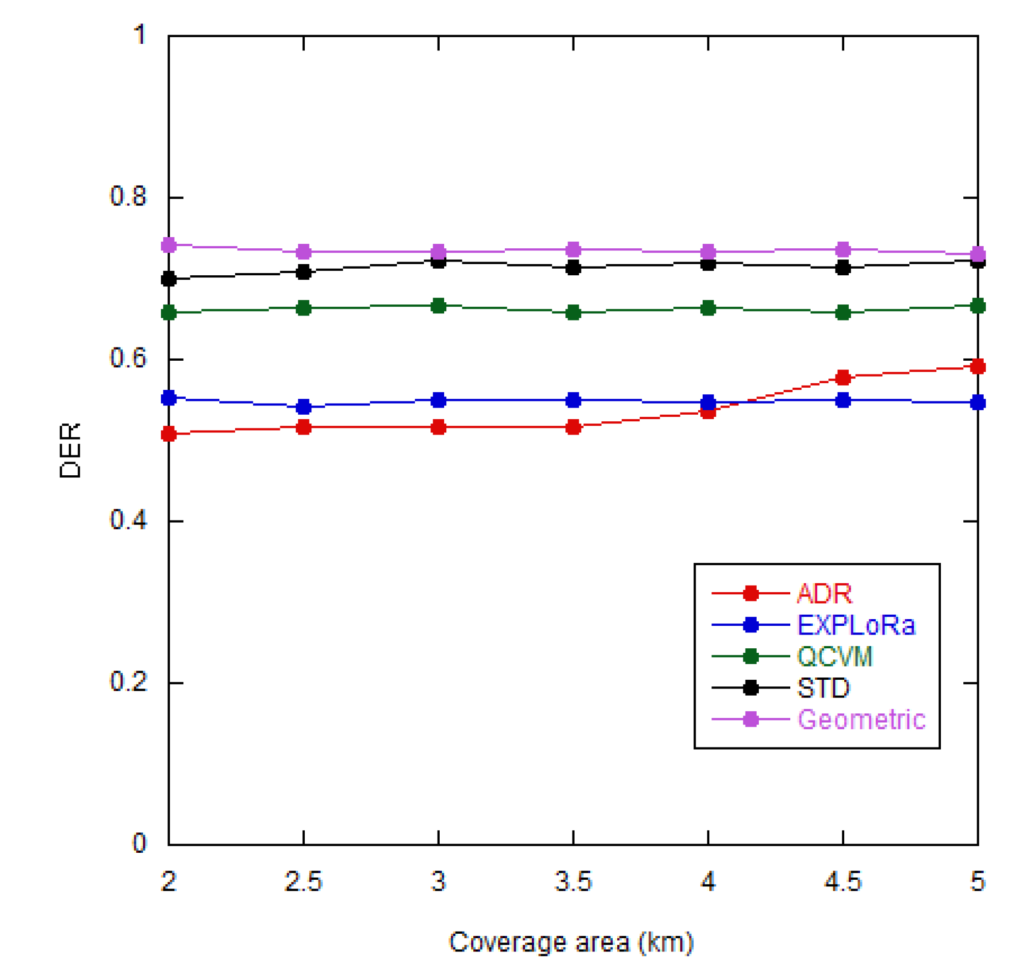
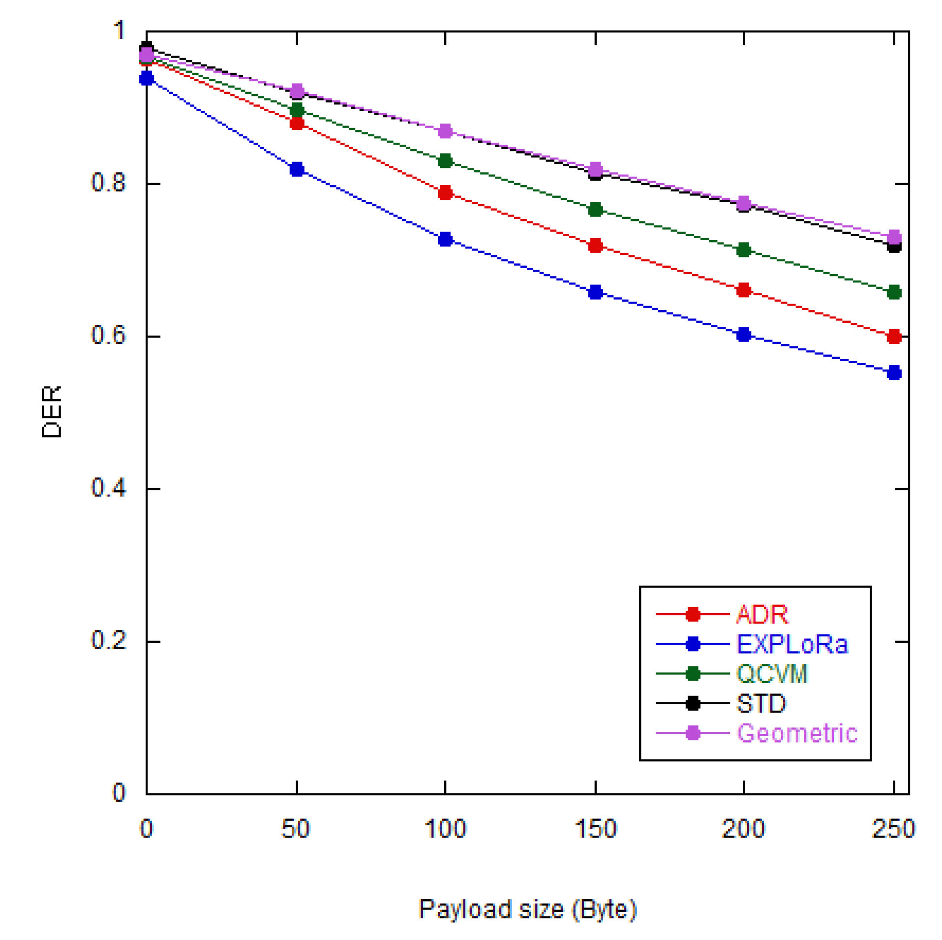
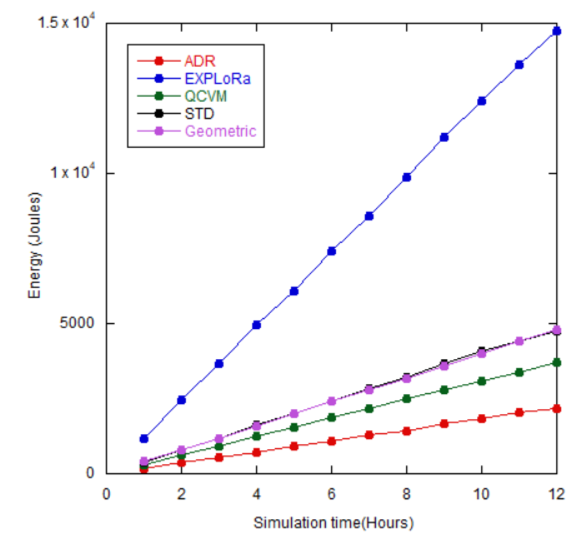
Expanding the coverage area and increasing the package size further underscored the efficacy of the proposed algorithm, consistently yielding the highest DER values. However, it was important to note that achieving these improvements required allowing higher energy consumption since larger SF values were also assigned.
Looking ahead, the GD algorithm emerges as a valuable tool for resource allocation, especially in scenarios, where there are mostly the same SF nodes in one area. This algorithm holds promise for optimizing resource distribution and finding the most efficient pathways. Furthermore, the application of this algorithm extends beyond LoRaWAN to other wireless communication technologies, including Sigfox, Wi-Fi, and 5G. The adaptability and effectiveness of the geometric distribution algorithm position it as a potential solution for future advancements in long range wireless communication optimization.
Figure 1.
Relationship of SF, data rate, airtime, energy, and sensitivity level.
Figure 1.
Relationship of SF, data rate, airtime, energy, and sensitivity level.
Figure 3.
Uniform random node pattern.
Figure 3.
Uniform random node pattern.
Figure 4.
Fixed node pattern.
Figure 4.
Fixed node pattern.
Figure 5.
The probability of success from the GD PMF at (a) p = 0.8, (b) p = 0.6, and (c) p = 0.2.
Figure 5.
The probability of success from the GD PMF at (a) p = 0.8, (b) p = 0.6, and (c) p = 0.2.
Figure 6.
GD algorithm-based SF assignment workflow.
Figure 6.
GD algorithm-based SF assignment workflow.
Figure 7.
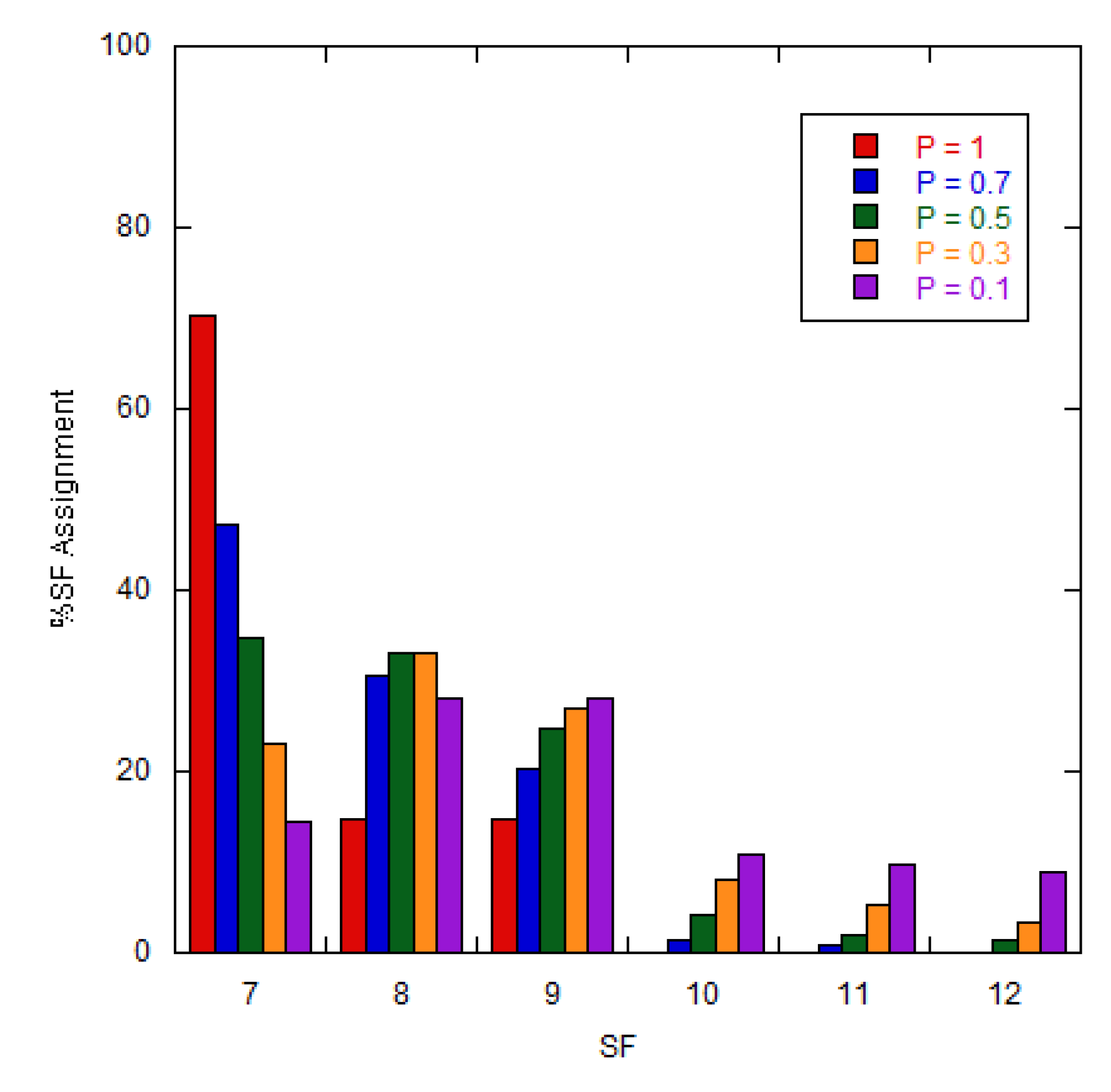
SF assignment for the uniform random pattern using the GD algorithm.
Figure 7.
SF assignment for the uniform random pattern using the GD algorithm.
Figure 8.
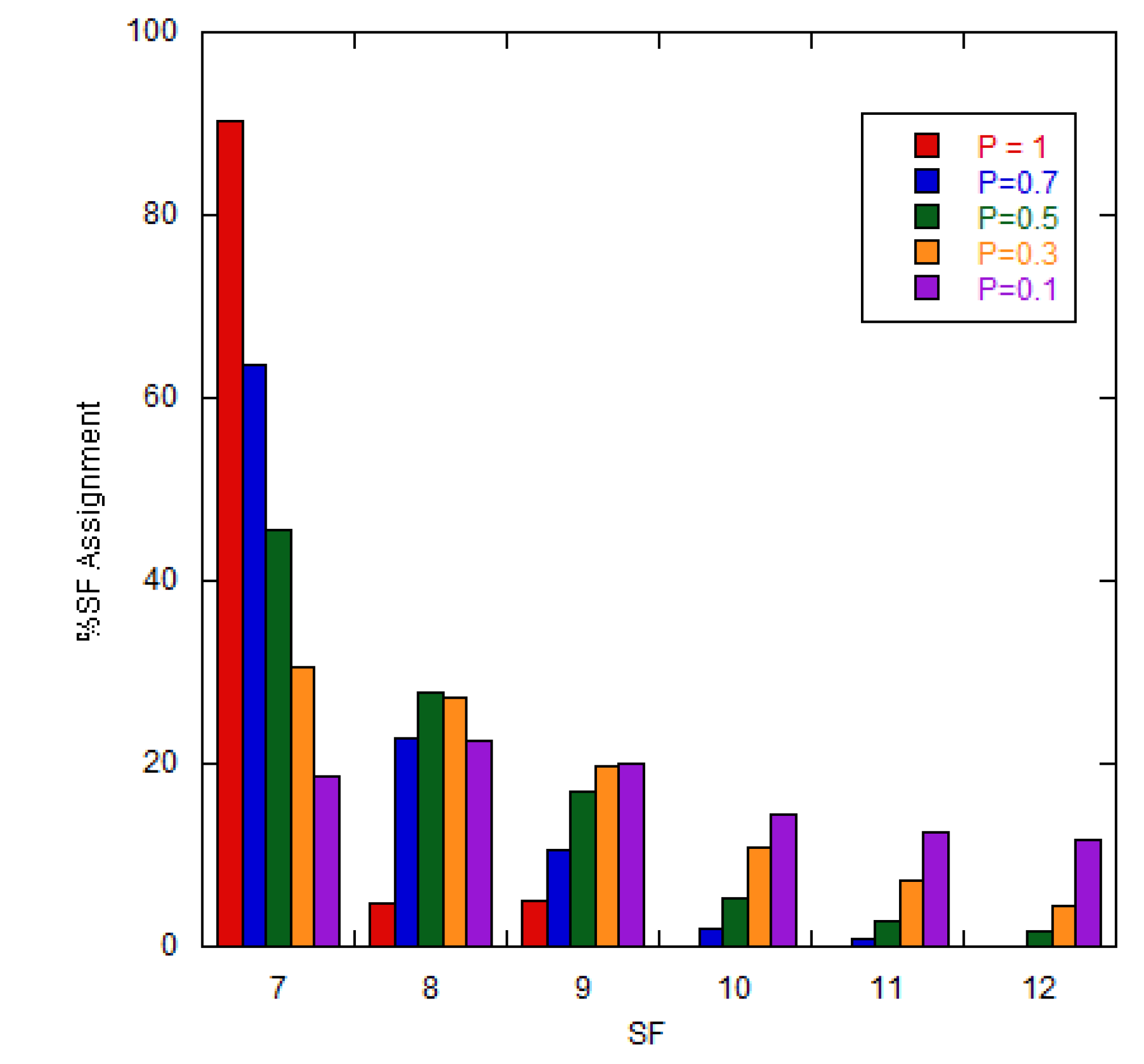
SF assignment for the fixed pattern using the GD algorithm.
Figure 8.
SF assignment for the fixed pattern using the GD algorithm.
Figure 9.
DER values after applying the GD algorithm to the fixed and uniform random patterns.
Figure 9.
DER values after applying the GD algorithm to the fixed and uniform random patterns.
Figure 10.
DER comparison between different algorithms for fixed and uniform random patterns.
Figure 10.
DER comparison between different algorithms for fixed and uniform random patterns.
Figure 11.
The DER values vs the coverage area for different algorithms.
Figure 11.
The DER values vs the coverage area for different algorithms.
Figure 12.
The DER values vs the payload size (Bytes) for different algorithms.
Figure 12.
The DER values vs the payload size (Bytes) for different algorithms.
Figure 13.
Energy consumptions from 1 hour to 12 hours of simulation time for different algorithms.
Figure 13.
Energy consumptions from 1 hour to 12 hours of simulation time for different algorithms.
Table 1.
The DER of the original ADR for the uniform random and fixed node patterns.
Table 1.
The DER of the original ADR for the uniform random and fixed node patterns.
| Coverage area |
Pattern |
%SF7 |
%SF8 |
%SF9 |
%SF10 |
%SF11 |
%SF12 |
DER Value |
| 2 km |
Uniform
random |
100.00 |
0.00 |
0.00 |
0.00 |
0.00 |
0.00 |
0.514 |
| Fixed |
100.00 |
0.00 |
0.00 |
0.00 |
0.00 |
0.00 |
0.510 |
| 3 km |
Uniform
random |
100.00 |
0.00 |
0.00 |
0.00 |
0.00 |
0.00 |
0.512 |
| Fixed |
100.00 |
0.00 |
0.00 |
0.00 |
0.00 |
0.00 |
0.514 |
| 4 km |
Uniform
random |
87.60 |
12.40 |
0.00 |
0.00 |
0.00 |
0.00 |
0.600 |
| Fixed |
96.53 |
3.47 |
0.00 |
0.00 |
0.00 |
0.00 |
0.538 |
| 5 km |
Uniform
random |
70.33 |
15.40 |
14.27 |
0.00 |
0.00 |
0.00 |
0.676 |
| Fixed |
89.53 |
4.93 |
5.53 |
0.00 |
0.00 |
0.00 |
0.589 |
Table 2.
The resulting set of weight factor (w) with p-value = 1 to 0.1.
Table 2.
The resulting set of weight factor (w) with p-value = 1 to 0.1.
|
p-value |
w1 |
w2 |
w3 |
w4 |
w5 |
w6 |
| 1 |
1 |
0 |
0 |
0 |
0 |
0 |
| 0.9 |
0.90 |
0.09 |
0.01 |
0.00 |
0.00 |
0.00 |
| 0.8 |
0.80 |
0.16 |
0.03 |
0.01 |
0.00 |
0.00 |
| 0.7 |
0.70 |
0.21 |
0.06 |
0.02 |
0.01 |
0.00 |
| 0.6 |
0.60 |
0.24 |
0.10 |
0.04 |
0.02 |
0.01 |
| 0.5 |
0.51 |
0.25 |
0.13 |
0.06 |
0.03 |
0.02 |
| 0.4 |
0.42 |
0.25 |
0.15 |
0.09 |
0.05 |
0.03 |
| 0.3 |
0.34 |
0.24 |
0.17 |
0.12 |
0.08 |
0.06 |
| 0.2 |
0.27 |
0.22 |
0.17 |
0.14 |
0.11 |
0.09 |
| 0.1 |
0.21 |
0.19 |
0.17 |
0.16 |
0.14 |
0.13 |
Table 3.
Simulation parameters.
Table 3.
Simulation parameters.
| Parameter |
Value |
| Number of nodes |
1,500 |
| Number of gateway |
1 |
| Node transmitted power |
14 dBm |
| Simulation time |
43,200 sec (12 Hours) |
| Average sending message time |
1,800 sec (30 minutes) |
| Bandwidth |
125 kHz |
| Frequency (AS923) |
923 MHz |
| Path-loss model |
Suburban Hata-Okumura |
| Payload size |
255 bytes |
| Coverage area |
5 km |
Table 4.
SF allocation from the GD algorithm at p = 0.5, default ADR scheme, and previous algorithms for the uniform random pattern.
Table 4.
SF allocation from the GD algorithm at p = 0.5, default ADR scheme, and previous algorithms for the uniform random pattern.
| Algorithm |
%SF7 |
%SF8 |
%SF9 |
%SF10 |
%SF11 |
%SF12 |
| Default ADR |
70.00 |
16.53 |
13.47 |
0.00 |
0.00 |
0.00 |
| EXPLoRa |
16.67 |
16.67 |
16.67 |
16.67 |
16.67 |
16.67 |
| QCVM |
33.40 |
33.40 |
33.20 |
0.00 |
0.00 |
0.00 |
| SD |
25.60 |
37.47 |
14.27 |
14.47 |
6.33 |
1.87 |
GD
(p = 0.5) |
34.73 |
33.13 |
24.60 |
4.07 |
2.07 |
1.40 |
Table 5.
SF allocation from the GD algorithm at p = 0.5, default ADR scheme, and previous algorithms for the fixed pattern.
Table 5.
SF allocation from the GD algorithm at p = 0.5, default ADR scheme, and previous algorithms for the fixed pattern.
| Algorithm |
%SF7 |
%SF8 |
%SF9 |
%SF10 |
%SF11 |
%SF12 |
| Default ADR |
89.67 |
5.40 |
4.93 |
0.00 |
0.00 |
0.00 |
| EXPLoRa |
16.67 |
16.67 |
16.67 |
16.67 |
16.67 |
16.67 |
| QCVM |
33.40 |
33.40 |
33.20 |
0.00 |
0.00 |
0.00 |
| SD |
35.20 |
32.73 |
17.33 |
12.67 |
1.33 |
0.73 |
GD
(p = 0.5) |
45.53 |
27.67 |
16.93 |
5.40 |
2.67 |
1.80 |
