Submitted:
25 July 2024
Posted:
25 July 2024
You are already at the latest version
Abstract
Keywords:
1. Introduction
2. Materials and Methods
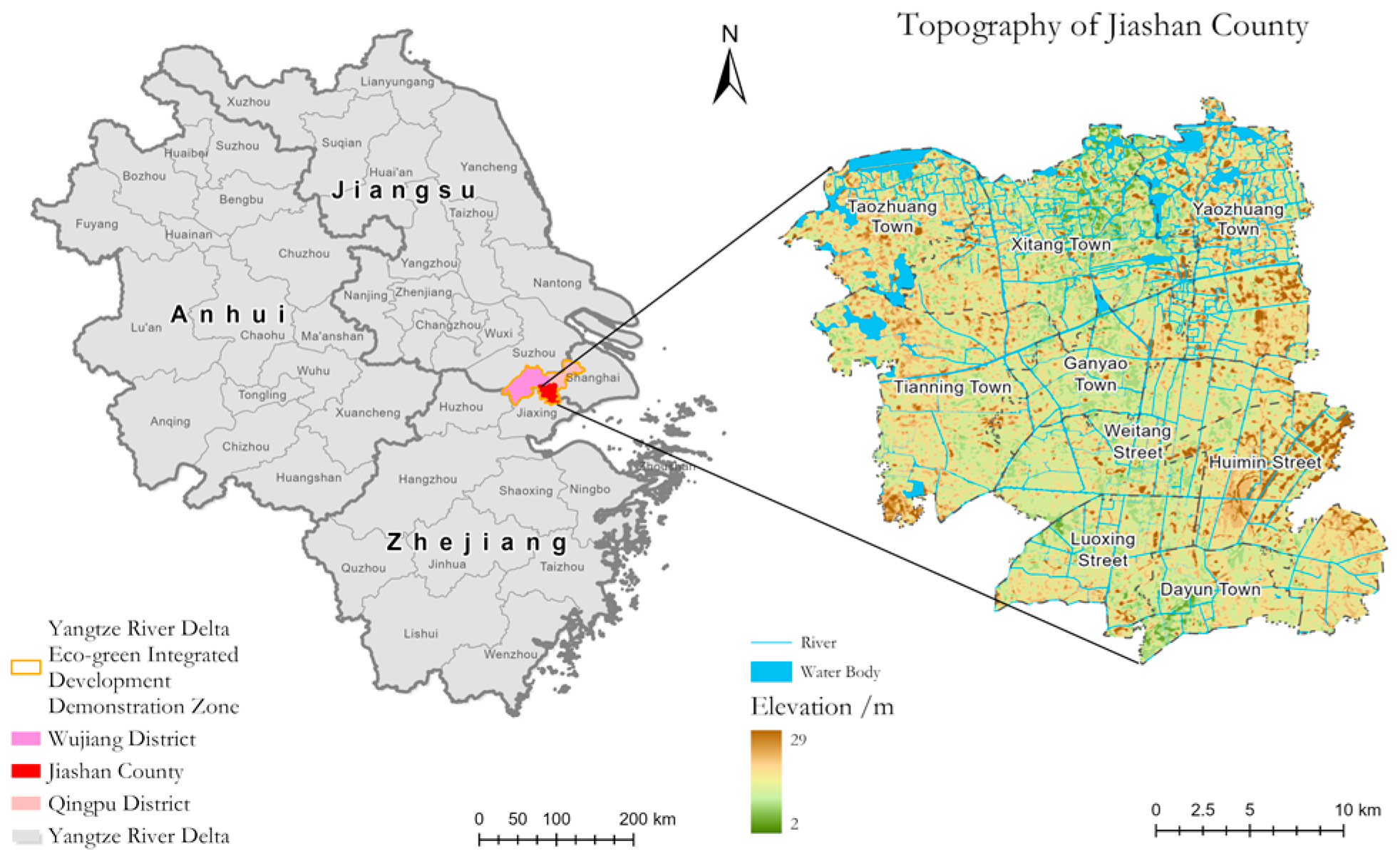
2.1. Study Area
2.2. Basis of Classification of Suburban Rural Landscape Functions
2.2.1. Rural Landscape Production Function
2.2.2. Rural Landscape Life Function
2.2.3. Ecological Function of Rural Landscape
2.3. Design of Rural Landscape Function Evaluation Index
2.4. Research Methods
2.4.1. Single Function Evaluation Of Landscape
2.4.2. Quantification of The Landscape Production-Living-Ecological Functions Trade-Offs And Synergistic Relationship
2.4.3. Spatial trade-off and synergistic relationship of the landscape production-living-ecological functions
2.5 Research Data
3. Results
3.1. Rural Landscape Function Evaluation Results
3.2. Temporal Evolution of The Function Trade-Off And Synergistic Relationship Of The Production-Living-Ecological Functions Of The Landscape
3.2.1. Temporal Pattern of Rural Landscape Synergy in Jiashan County
3.2.2. Temporal Pattern of Rural Landscape Trade-Off in Jiashan County
3.2.3. Temporal Pattern of the Transformation Of The Rural Landscape Trade-Off And Synergistic Relationship in Jiashan County
3.2.4. Temporal Pattern of the Rural Landscape Compatibility in Jiashan County
3.3. Analysis of the spatial evolution of the tradeoff and synergistic relationship between the landscape production-living-ecological functions
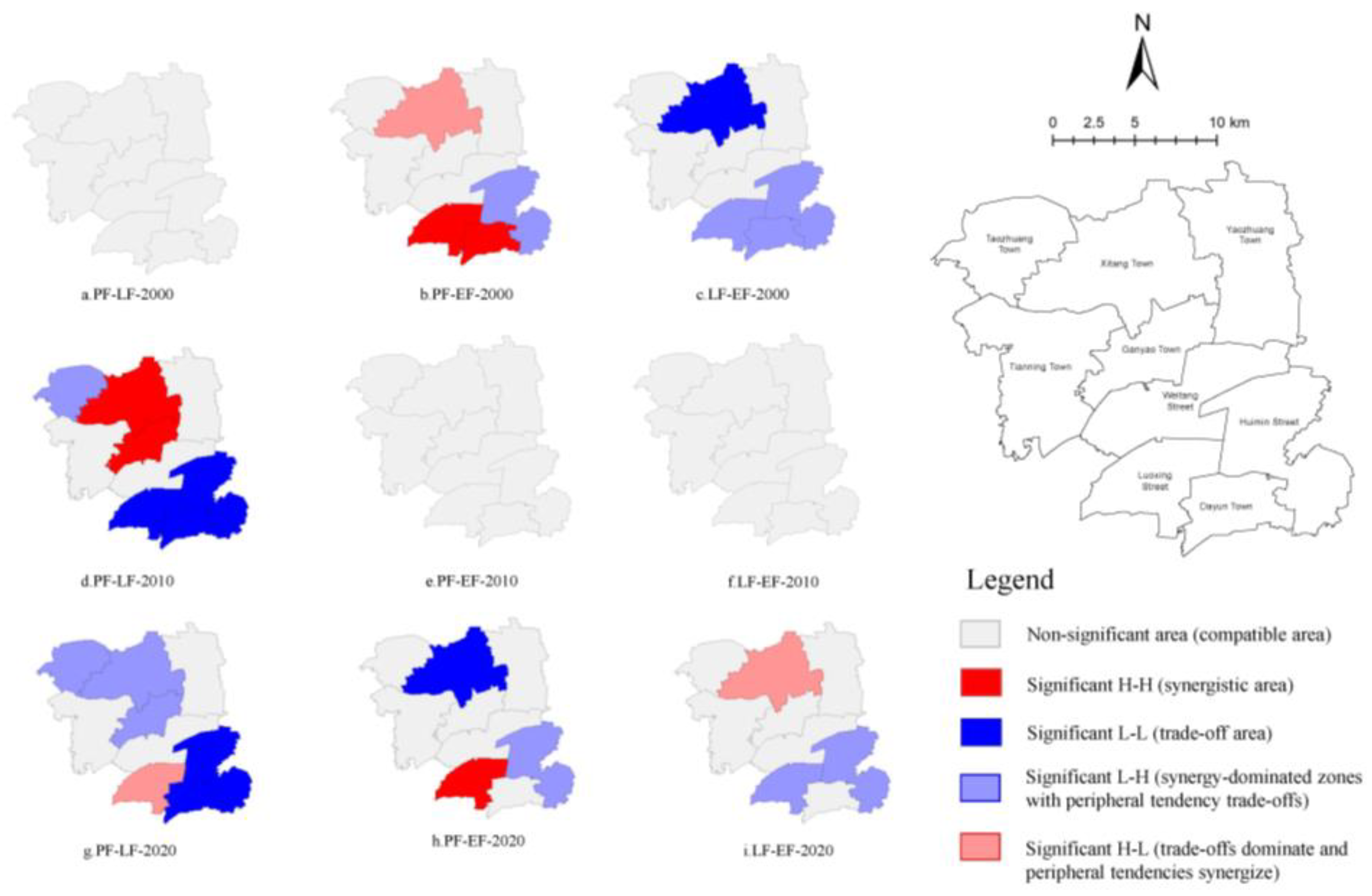
3.3.1. Spatial Pattern of the Trade-Off And Synergistic Relationship Of The Production-Living-Ecological Functions In The Rural Landscape
3.3.2. Spatiotemporal Evolution of the Trade-Off And Synergy Between The Production, Life, And Ecological Functions
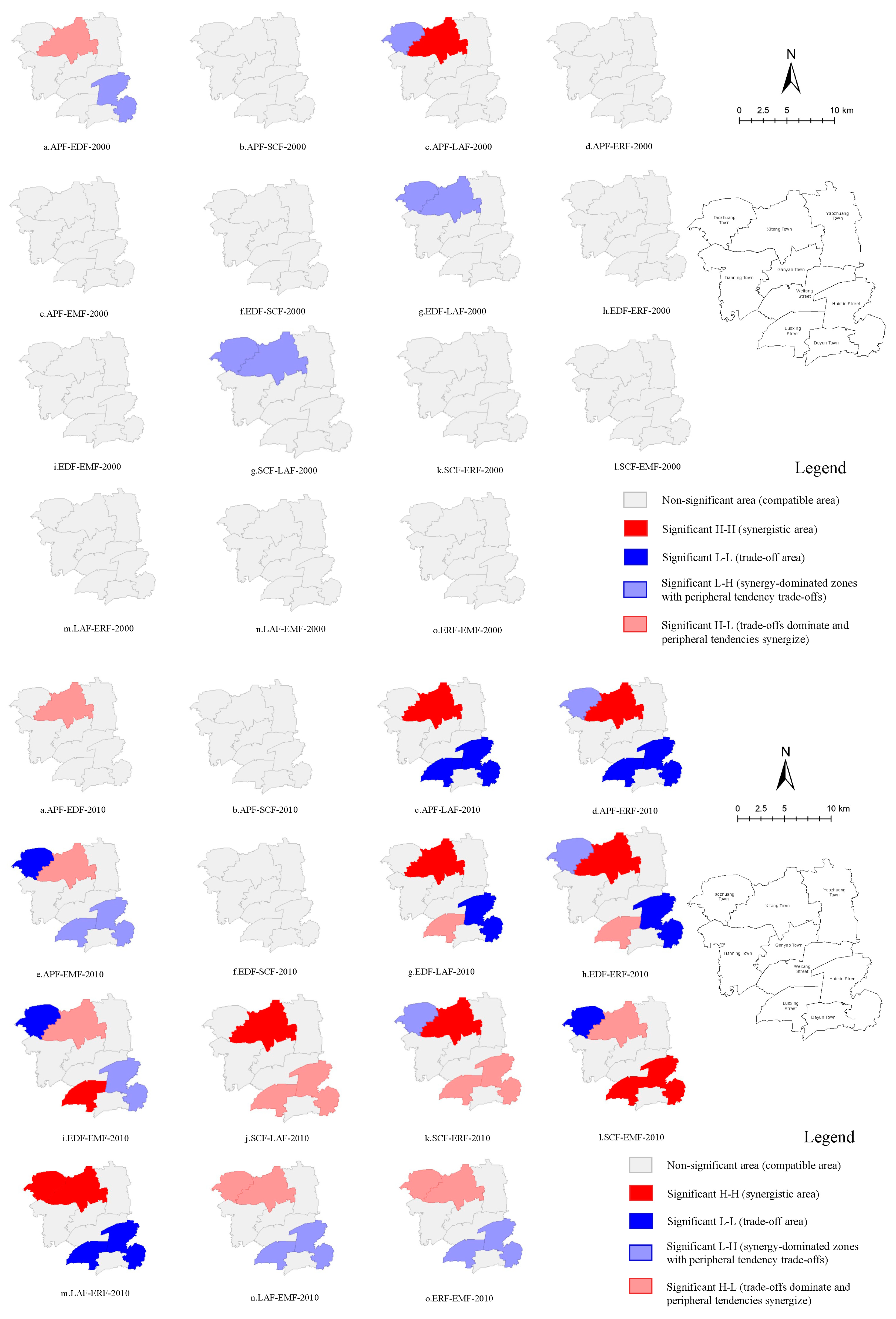
3.3.3. Trade-Offs Between Sub-Functions -Spatiotemporal Evolution of Synergistic Relationships
4. Discussion
5. Conclusions
6. Limitations
Author Contributions
Funding
Data Availability Statement
Conflicts of Interest
References
- Willemen, L.; Hein, L.; Vanmensvoort, E.F.; Verburg, P.H. Space for people, plants, and livestock? Quantifying interactions among multiple landscape functions in a Dutch rural region. Ecol. Indic.2010, 10, 62-73. [CrossRef]
- Fischer, J.; Lindenmayer, D.B. Landscape modification and habitat fragmentation: A synthesis. Glob. Ecol. Biogeogr. 2007, 16, 265-280. [CrossRef]
- Yang, G.; Ge, Y.; Xue, H.; Yang, W.; Shi, Y. Using ecosystem service bundles to detect trade-offs and synergies across urban-rural complexes. Landsc. Urban Plan. 2015, 136, 110-121. [CrossRef]
- Qiu, J.X.; Turner, M.G. Spatial interactions among ecosystem services in an urbanizing agricultural watershed. Proc. Natl. Acad. Sci. USA 2013, 110, 12149-12154. [CrossRef]
- Chen, X.; Ning, Y. A study on rural urbanization in the suburbs of big cities: A case study of Shanghai. Urban Probl. 1997, 3, 27-31.
- Yin, W. Theoretical and Practical Exploration of metropolitan suburb development. Master’s Thesis, East China Normal University, Shanghai, China, 2007.
- Zheng, J.; Na, L.; Liu, B.; Zou, Y. An ecological service system based study on suburban rural landscape multifunction. Land 2021, 10, 232. [CrossRef]
- Jiang, J. Research on the organic rural renewal strategy of super-city suburbs under the urban-rural integration pattern: A case study of Shanghai’s suburbs and exurbs. Shanghai Urban Plan. Rev. 2023, 4, 62-69.
- Peng, J.; Liu, Z.; Liu, Y.; Hu, Y.; Wang, Y. Multifunctionality assessment of urban agriculture in Beijing City, China. Sci. Total Environ. 2015, 537, 343-351. [CrossRef]
- Lautenbach, S.; Kugel, C.; Lausch, A.; Seppelt, R. Analysis of historic changes in regional ecosystem service provisioning using land use data. Ecol. Indic. 2011, 11, 676-687. [CrossRef]
- Skalos, J.; Berchova, K.; Pokorny, J.; Vozenilek, V. Landscape water potential as a new indicator for monitoring macrostructural landscape changes. Ecol. Indic. 2015, 36, 80-93. [CrossRef]
- Costanza, R.; Diarge, R. The value of the world’s ecosystem services and natural capital. Nature 1997, 387, 253-260. [CrossRef]
- Zhu, Q.; Hu, W.; Zhao, Z. Dynamic analysis of trade-off and synergistic spatio-temporal pattern of cultivated land "three crops" function: A case study of Hubei Province. Econ. Geogr. 2018, 38, 143-153.
- De Groot, R.S.; Wilson, M.A.; Boumans, R.M.J. A typology for the classification, description and valuation of ecosystem function, goods and services. Ecol. Econ. 2010, 41, 393-408. [CrossRef]
- Cai, Y. Rural transformation and farmland protection mechanism in China. Sci. Geogr. Sin. 2001, 21, 1-6.
- Gonzalez-Redin, J.; Luque, S.; Poggio, L.; Smith, R.; Gimona, A. Spatial Bayesian belief networks as a planning decision tool for mapping ecosystem services trade-offs on forested landscapes. Environ. Res. 2016, 144, 15-26. [CrossRef]
- Deng, R. Research on landscape planning and design of terrace based on the integration of agriculture and tourism -- A case study of Huayan Terrace in Youyang. Master’s Thesis, Southwest University, Chongqing, China, 2008.
- Zou, H. Assessment of ecosystem service value of shrub grass in hilly and gully region of the Loess Plateau in Longzhong. Master’s Thesis, Lanzhou University, Lanzhou, China, 2021.
- Zhang, D.; Li, K.; Sun, Q.; Wang, Y. Analysis of site community characteristics and landscape function in semi-arid area of Loess Plateau. Chin. Urban For. 2017, 15, 11-15.
- Luo, S.; Lai, Q.; Wang, X.; Chen, X. Cultivated land zoning control in Fujian Province based on the function evaluation and trade-off synergy relationship of "production-living-ecology". Trans. Chin. Soc. Agric. Eng. 2019, 39, 271-280.
- Zhuo, Z.; Xing, A.; Sun, Z.; Gao, L. Analysis of synergistic development and trade-off of agro-ecosystems in Northeast China. Chin. J. Eco-Agric. 2018, 26, 892-902.
- Feng, Z.; Wu, J.; Gao, Y.; Yuan, S. Landscape function classification based on SOFM network: A case study of Beijing and its surrounding areas. J. Geoinf. Sci. 2012, 14, 800-806.
- Ren, G.; Liu, L.; Li, H.; Zhang, X.; Yang, L. Evolution of function trade-off and synergistic relationship of rural landscape in urban suburbs. Trans. Chin. Soc. Agric. Eng. 2019, 35, 273-285.
- The CPC Central Committee, The State Council. CPC Central Committee. The State Council issued the Yangtze river delta regional integration development plan outline. Available online: http://www.gov.cn/zhengce/zhengceku/2023-02/21/content_5742406.htm (accessed on 4 February 2023).
- Shanghai Municipal Government Synergy and Exchange Office. Shanghai what do together into neighboring event. Available online: http://www.gov.cn/zhengce/zhengceku/2023-02/21/content_5742406.htm (accessed on 10 February 2021).
- Under the State Council. The overall plan for the Yangtze River Delta eco-green integrated development demonstration zone (2021-2035). Available online: http://www.gov.cn/zhengce/zhengceku/2023-02/21/content_5742406.htm (accessed on 4 February 2023).
- Ji, S.; Duan, J.; Xue, S.; Zhang, J. Exploration of urban design methods based on spatial gene inheritance: A case study of the living room of Shui Township in Yangtze River Delta integrated Demonstration Zone. City Plan. Rev. 2019, 47, 4-12+48.
- Wang, C.; Peng, Q.; Tang, N.; Li, J.; Wang, X. Spatial and temporal evolution, synergy and tradeoff of cultivated land "production-living-ecological" function from 2005 to 2015: A case study of Shapingba District, Chongqing. Sci. Geogr. Sin. 2018, 38, 590-599.
- Pan, J.; Li, Z. Spatial trade-off and synergistic effect of ecosystem services in arid inland river basin. Trans. Chin. Soc. Agric. Eng. 2017, 33, 280-289.
- Fan, J. Plan of main function zoning in China. Acta Geogr. Sin. 2015, 70, 186-201.
- Millennium E.A. Ecosystems and Human Well-being Synthesis. Washington DC: Island Press, 2005; pp. 559-567.
- Cheng, Z.; Zhang, Y.; Wang, L.; Song, L. Study on the spatial evolution characteristics and driving forces of "production-living-ecology" in western Jilin Province. Areal Res. Dev. 2023, 42, 33-39.
- Wei, W.; Yin, L. Evolution and driving mechanism of "three-region spatial pattern" in Northeast China. Sci. Geogr. Sin. 2023, 43, 324-336.
- Li, W.; Wang, F.; Ma, X.; Xiao, L.; Lin, Y. Spatial and temporal evolution mechanism of land use in ecotype urban tourism complex: A case study of Xixi Wetland. Tour. Trib. 2019, 38, 133-148.
- Xu, X.; Liu, J.; Zhang, S.; Ouyang, Z.; Zheng, D. China Multi-Period Land Use and Land Cover Remote Sensing Monitoring Data Set (CNLUCC). Available online: http://www.resdc.cn (accessed on 23 February 2024).
- Van Donkelaar, A.; Hammer, M.S.; Bindle, L.; Brauer, M.; Martin, R.V. Monthly Global Estimates of Fine Particulate Matter and Their Uncertainty. Environ. Sci. Technol. 2021, 55, 15287-15300. [CrossRef]
- WORLDPOP; Bondarenko, M. Individual Countries 1km UN Adjusted Population Density (2000-2020). Available online: https://hub.world pop.org/project/categories?id=18 (accessed on 6 February 2024).
- Li, G.; Fang, C. Quantitative identification and analysis of urban ecology-Production-living spatial function. Acta Geogr. Sin. 2016, 71, 49-65.
- Mina, M.; Bugmann, H.; Cordonnier, T.; Irauschek, F.; Klopcic, M.; Cailleret, M. Future ecosystem services from European mountain forests under climate change. J. Appl. Ecol. 2017, 54, 389-401. [CrossRef]
- Peng, J.; Lu, H.; Liu, Y.; Hu, Y.; Li, W.; Wu, J. Research progress and prospect of "production-living-ecological" functional landscape at home and abroad. Adv. Earth Sci. 2015, 30, 465-476.
- Green, R.E.; Cornell, S.J.; Scharlemann, J.P.W.; Balmford, A. Farming and the fate of wild nature. Science 2005, 307, 550-555. [CrossRef]
| Target Layer | Criterion Layer | Index Layer | Calculation Method or Index Significance | Index Relationship | Index Weight |
|---|---|---|---|---|---|
| Production function (PF) | Agricultural production function (APF) |
Agricultural productivity per capita | Gross value of primary industry/total township population (10,000 yuan/person). | Forward direction | 6.02% |
| Agricultural output value per land | Agricultural output value/cultivated land area (Yuan/square meter). | Forward direction | 4.53% | ||
| Economic development function (EDF) |
Industrial contribution rate | (Output value of primary industry + output value of tertiary industry)/township GDP. | Forward direction | 10.94% | |
| Township urbanization level | Township construction land/total area of township. | Forward direction | 5.39% | ||
| Living function (LF) |
Space carrying function (SCF) | Per capita living area | Township construction land area/total population (km2). | Forward direction | 7.25% |
| Population density | Reflects the population carrying capacity of the township. | Forward direction | 12.27% | ||
| Landscape aesthetic function (LAF) | Landscape connectivity | CONTAG (0, 100%] - The degree of agglomeration or spread of different patch types in the landscape. The greater the value is, the better the patch connectivity is. | Forward direction | 6.44% | |
| Landscape diversity | SHDI [0, +∞) - The larger the value is, the more abundant the patch types and distributions in the landscape. | Forward direction | 5.60% | ||
| Ecological function (EF) |
Ecological regulation function (ERF) | NDVI | Reflect the vegetation state of the township. | Forward direction | 23.91% |
| Ecological synergy degree | SHEI [0, 1) - A smaller value indicates that the landscape is more dominated by a few dominant types, and a larger value indicates that the distribution of all of the landscape types is more uniform. | Forward direction | 5.80% | ||
| Environmental maintenance function (EMF) | PM2.5 | Reflects the degree of air pollution in towns and villages. | Reverse direction | 4.32% | |
| Landscape fragmentation | The landscape division Index is one of the indicators used to evaluate landscape fragmentation, and it mainly measures the degree of fragmentation of views. | Reverse direction | 7.54% |
| Data | Data Source | Application Indicators |
|---|---|---|
| Multi-period land use/land cover remote sensing monitoring data for China [35] | The multi-period land use/land cover remote sensing monitoring Chinese National Land Use and Cover Change (CNLUCC) database from the Chinese Academy of Sciences has a resolution of 30 m. | Landscape connectivity, landscape diversity index, and landscape fragmentation |
| Satellite-derived PM2.5 [36] | The global and regional PM2.5 concentrations are estimated using information from satellite, modelling, and monitoring sources. The aerosol optical depth and simulation [Goddard Earth Observing System with Chemistry (GEOS-Chem)] from multiple satellites (MODIS, VIIRS, MISR, and SeaWiFS) and their respective retrievals (Dark Target, Deep Blue, and MAIAC) are combined to determine the relative uncertainties based on observations using ground-based solar photometers [Aerosol Robotic Network (AERONET)] to produce geophysical estimates. This explains most of the differences in ground-level PM2.5 measurements. Additional information from PM2.5 measurements is then tallied at a resolution of 0.01°. | PM2.5 |
| GDP | The China km grid GDP spatial distribution dataset from the Resources and Environmental Sciences Data Registration and Publication System, Chinese Academy of Sciences (http://www.resdc.cn/DOI). | GDP |
| Population density [37] | China’s 1 km population density dataset was downloaded from WorldPop (https://hub.worldpop.org/). | Population density |
| Normalized Difference Vegetation Index (NDVI) | Landsat 7 and Landsat 8 images with a resolution of 30 m were downloaded from NASA, and the NDVI index was calculated in ArcGIS Pro (https://www.jiashan.gov.cn/). | NDVI |
| Administrative boundary data | The base map is from the standard map service system of the Ministry of Natural Resources, and the review number is GS(2023)2767. | \ |
| Jiashan County Yearbook for 2001, 2011, and 2021 | Jiashan County Statistics Bureau for (https://www.jiashan.gov.cn/). | Agricultural earnings, industrial output, and commercial activity |
| Category | Feature | 2000 | 2010 | 2020 |
|---|---|---|---|---|
| Target layer | PF | 0.043 | 0.091 | 0.108 |
| LF | 0.070 | 0.143 | 0.152 | |
| EF | 0.310 | 0.087 | 0.102 | |
| Criterion layer | APF | 0.020 | 0.050 | 0.052 |
| EDF | 0.023 | 0.041 | 0.056 | |
| SCF | 0.039 | 0.064 | 0.075 | |
| LAF | 0.031 | 0.077 | 0.079 | |
| ERF | 0.242 | 0.039 | 0.039 |
| Rural Landscape Function Synergy Type | 2000 | 2010 | 2020 | |||
|---|---|---|---|---|---|---|
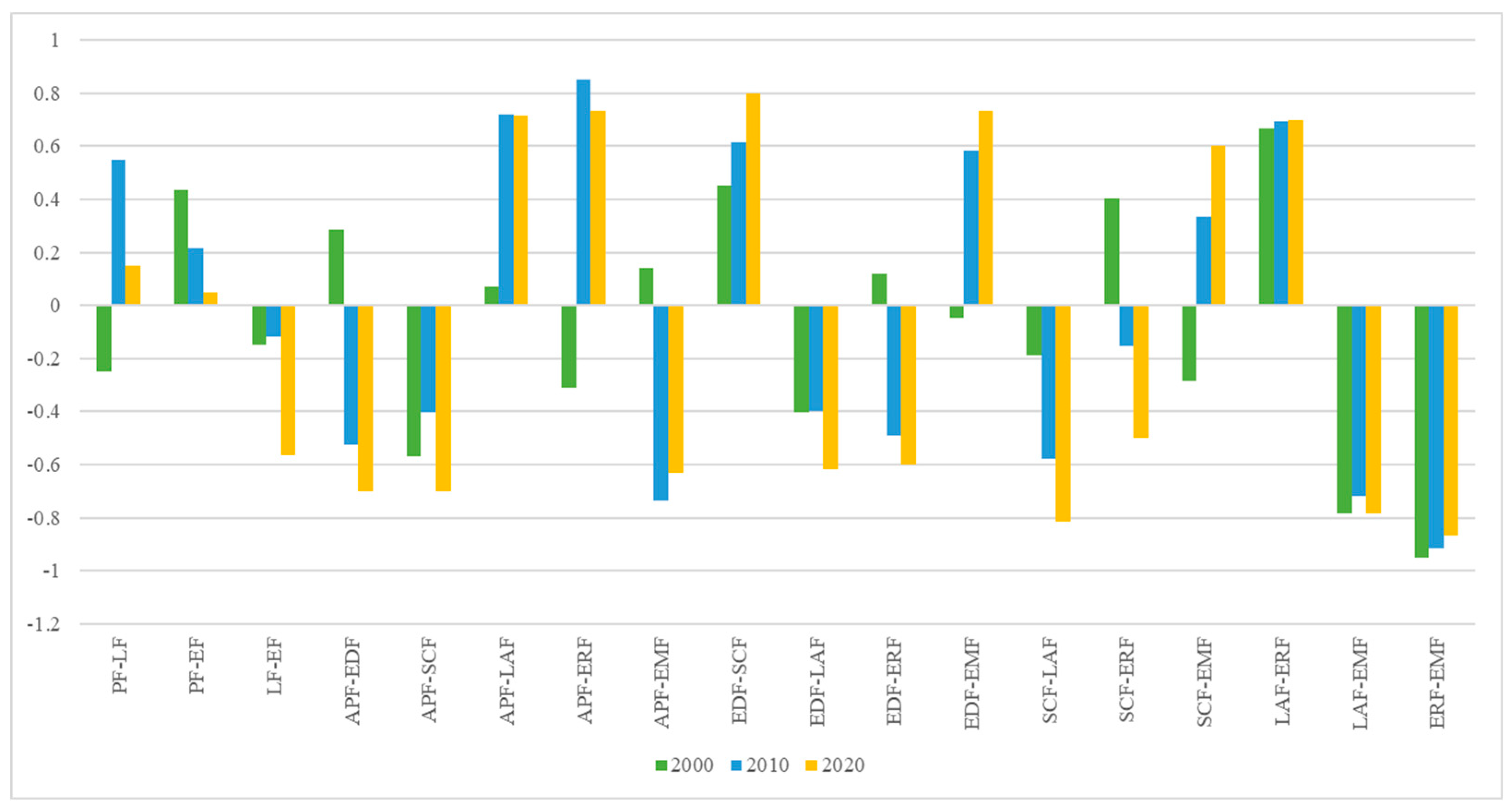
| Correlation Coefficient | P-Value | Correlation Coefficient | P-Value | Correlation Coefficient | P-Value | |
| PF-LF | −0.25 | 0.516 | 0.55 | 0.125 | 0.15 | 0.7 |
| PF-EF | 0.433 | 0.244 | 0.217 | 0.576 | 0.05 | 0.898 |
| LF-EF | −0.15 | 0.7 | −0.117 | 0.765 | −0.567 | 0.112 |
| APF-EDF | 0.286 | 0.493 | −0.527 | 0.145 | −0.700* | 0.036 |
| APF-SCF | −0.571 | 0.139 | −0.405 | 0.279 | −0.700* | 0.036 |
| APF-LAF | 0.071* | 0.008 | 0.720* | 0.029 | 0.717* | 0.03 |
| APF-ERF | −0.31* | 0.04 | 0.851** | 0.004 | 0.733* | 0.025 |
| APF-EMF | 0.143 | 0.736 | −0.736* | 0.024 | −0.633 | 0.067 |
| EDF-SCF | 0.452 | 0.26 | 0.613 | 0.079 | 0.800** | 0.01 |
| EDF-LAF | −0.405 | 0.32 | −0.4 | 0.286 | −0.617 | 0.077 |
| EDF-ERF | 0.119 | 0.779 | −0.492 | 0.179 | −0.6 | 0.088 |
| EDF-EMF | −0.048 | 0.911 | 0.583 | 0.099 | 0.733* | 0.025 |
| SCF-LAF | −0.19 | 0.651 | −0.58 | 0.102 | −0.817** | 0.007 |
| SCF-ERF | 0.405 | 0.32 | −0.154 | 0.693 | −0.5 | 0.17 |
| SCF-EMF | −0.286 | 0.493 | 0.336 | 0.376 | 0.6 | 0.088 |
| LAF-ERF | 0.667 | 0.071 | 0.695* | 0.038 | 0.700* | 0.036 |
| LAF-EMF | −0.786* | 0.021 | −0.717* | 0.03 | −0.783* | 0.013 |
| ERF-EMF | −0.952** | 0 | −0.915** | 0.001 | −0.867** | 0.002 |
| Rural Landscape Function Synergy Type | 2000 | 2010 | 2020 | |||
|---|---|---|---|---|---|---|
| Moran’s I | Z-Value | Moran’s I | Z-Value | Moran’s I | Z-Value | |
| PF-LF | −0.0863 | −1.0237 | 0.3171 | 2.2568 | −0.1111 | −0.6131 |
| PF-EF | 0.1299 | 1.1015 | −0.0957 | −0.3133 | 0.111 | 0.6636 |
| LF-EF | −0.2152 | −1.5692 | 0.0288 | −0.0399 | −0.3997 | −2.7636 |
| APF-EDF | −0.1333 | −0.424 | 0.1815 | 0.7392 | 0.0323 | −0.2552 |
| APF-SCF | 0.0059 | −0.3166 | 0.0097 | −0.2245 | 0.0652 | 0.0348 |
| APF-LAF | −0.0398 | −1.6717 | 0.2665 | 1.8745 | 0.2243 | 1.6523 |
| APF-ERF | 0.0104 | −0.3515 | 0.2062 | 1.5868 | 0.1796 | 1.3963 |
| APF-EMF | −0.0047 | 0.3975 | −0.141 | −1.2271 | −0.179 | −1.397 |
| EDF-SCF | −0.0227 | 0.0049 | −0.1681 | −0.5528 | −0.0477 | 0.2823 |
| EDF-LAF | −0.1692 | −1.3248 | 0.1249 | 0.4548 | −0.1605 | −1.4015 |
| EDF-ERF | −0.134 | −1.0232 | 0.159 | 0.6713 | −0.158 | −1.4562 |
| EDF-EMF | 0.156 | 1.1781 | −0.194 | −0.8462 | 0.169 | 1.4948 |
| SCF-LAF | 0.044 | 0.3829 | −0.052 | −0.6616 | −0.094 | −0.9531 |
| SCF-ERF | −0.0092 | 0.261 | −0.1226 | −1.0871 | −0.1343 | −1.206 |
| SCF-EMF | −0.0126 | −0.3724 | 0.1017 | 0.9138 | 0.1243 | 1.1151 |
| LAF-ERF | 0.178 | 1.6897 | 0.4774 | 2.7977 | 0.4597 | 2.7344 |
| LAF-EMF | −0.1937 | −1.6544 | −0.3953 | −2.4541 | −0.463 | −2.7251 |
| ERF-EMF | −0.0638 | −0.984 | −0.241 | −1.781 | −0.3482 | −2.2479 |
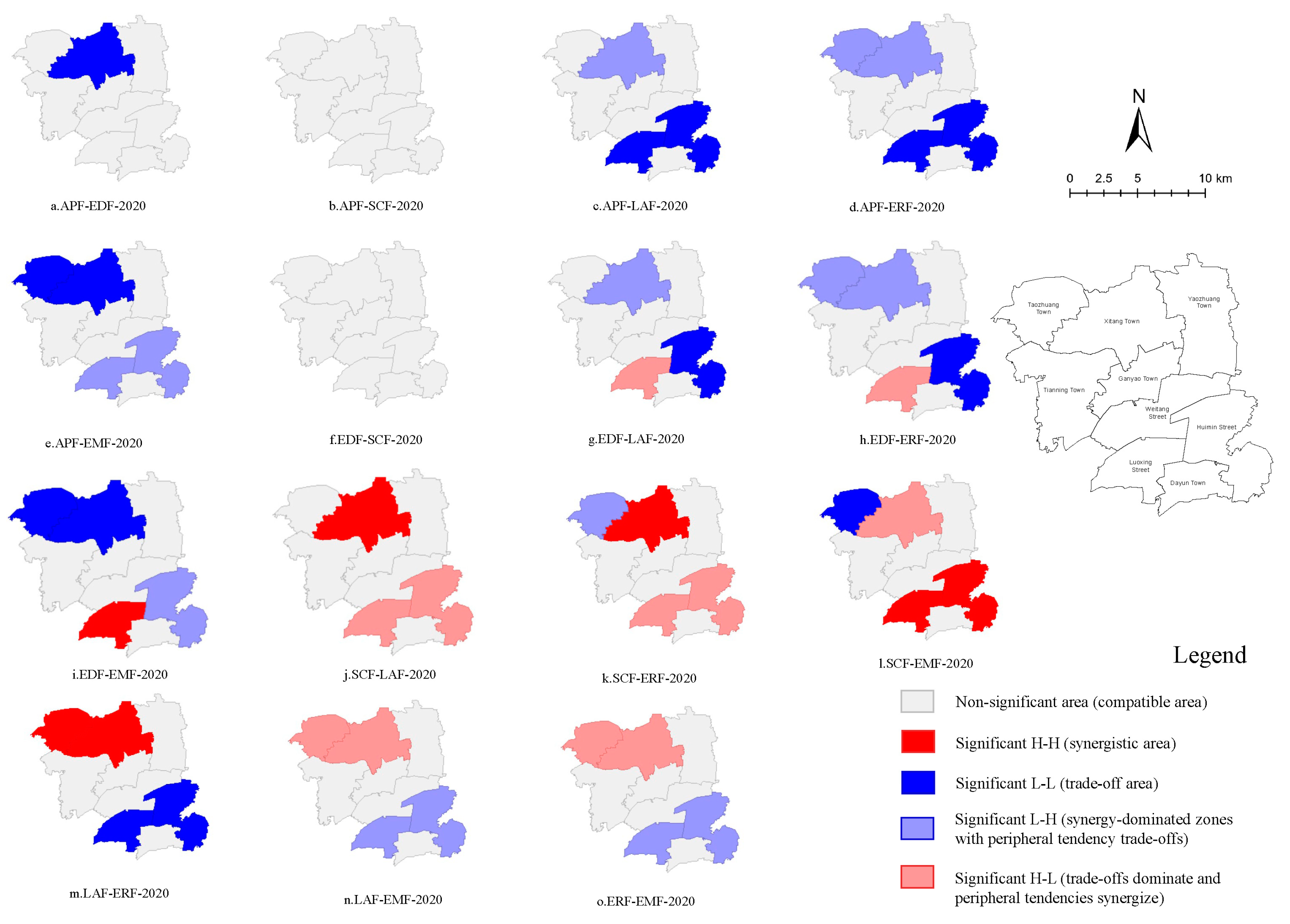
| Legend | Significance |
|---|---|
| Non-significant area (Compatible) | P > 0.05 indicates a non-significant region, that is, the function of the region is compatible. |
| Significant H-H region (Synergy) | P < 0.05 indicated a significant region, and there was synergy among the regional functions, as well as synergy in the surrounding areas, so the spatial heterogeneity was small and the relationship was stable. |
| Significant L-L region (Trade-off) | There were trade-offs between the regional functions, and the surrounding areas were also trade-offs, so the spatial heterogeneity was small and the relationship was stable. |
| Significant L-H region (Trade-off - peripheral region is synergistic) | The regional functions were trade-offs, but the surrounding areas were synergistic, so the spatial heterogeneity was large and the relationship was unstable. |
| Significant H-L region (Synergy-peripheral region as trade-off) | There was synergy among the regional functions, but the surrounding areas were trade-offs, so the spatial heterogeneity was large and the relationship was unstable. |
Disclaimer/Publisher’s Note: The statements, opinions and data contained in all publications are solely those of the individual author(s) and contributor(s) and not of MDPI and/or the editor(s). MDPI and/or the editor(s) disclaim responsibility for any injury to people or property resulting from any ideas, methods, instructions or products referred to in the content. |
© 2024 by the authors. Licensee MDPI, Basel, Switzerland. This article is an open access article distributed under the terms and conditions of the Creative Commons Attribution (CC BY) license (http://creativecommons.org/licenses/by/4.0/).


