1. Introduction
Explosions generate infrasonic (<20 Hz) and/or low frequency sounds (<300 Hz) that can travel vast distances. The travel distance and frequency range of these sounds depend on the size of the explosion and atmospheric conditions. For reference, the peak central frequency of a pressure wave from a 1 ton of trinitrotoluene (TNT) explosion would be around 6.3 Hz, and it would be around 63 Hz for a 1 kg TNT explosion [
1]. This phenomenon can and has been used to detect explosions. For example, the International Monitoring System (IMS) has a network of globally distributed infrasound sensors to detect large (>1 kiloton) explosion events [
2]. Similarly, for smaller yield explosions, there have been examples of infrasound and seismoacoustic sensors deployed on regional and local scales [
3,
4,
5,
6,
7,
8,
9]. However, as networks get denser, the cost and difficulty of covering a wider area grows rapidly. Thus, many of these networks are deployed temporarily for experiments or around specific areas of interest, such as volcanos or testing sites [
10] and optimized for the prevailing weather patterns.
The prompt detection of smaller yield explosions in key locations and regions could be crucial as fast and reliable detection would lead to decreased response times and could potentially reduce casualties and damage. However, as mentioned previously, having a dense sensor network for low yield explosions become expensive and difficult to maintain. A solution to this problem is using non-traditional sensors such as smartphones, especially considering recent advancements and success in mobile crowd sensing [
11,
12,
13]. Although there is still a need for more publicly available explosion dataset to train and design detection and classification models, several studies using smartphones for explosion detection have already laid some groundwork [
10,
14,
15,
16,
17]. We build off these initial studies by releasing labeled explosion data to the public and demonstrate the ability of current algorithms to detect and classify infrasonic signals.
The Smartphone High-explosive Audio Recordings Dataset (SHAReD) [
18], the labeled data that we collected on smartphone networks, provides a unique dataset that can be utilized for machine learning (ML) methods for explosion detection. The audio data from the high-explosive (HE) dataset were used in conjunction with data from an external environmental sound dataset (ESC-50 [
19]) to train two separate machine learning models, one using transfer learning (YAMNet [
20]) and the other considering only the low frequency content of the waveforms. These two models were then combined into an ensemble model to classify audio data as “explosion,” “ambient,” or “other.” Although the two models both performed well while classifying the sounds individually, each model had its own shortcomings in distinguishing between the categories. We found that by combining the two models into one ensemble model, the strengths of each model compensated for the shortcomings of the other, significantly improving performance.
Transfer Learning, YAMNet, and Ensemble Learning
Transfer learning (TL) is a machine learning technique which utilizes a pre-trained model as a starting point for a new model designed to perform a similar task. TL has gained popularity as it can compensate for the consequences of having a limited amount of data on which to train a model [
21]. TL using convolutional neural networks (CNNs), such as Google’s Yet Another Mobile Network (YAMNet), has become common practice for environmental sound classification [
22,
23,
24,
25].
YAMNet is an off-the-shelf machine learning model trained on data from AudioSet [
26], a dataset of over 2 million annotated YouTube audio clips, to predict 521 audio classes [
20]. It utilizes the Mobile_v1 architecture, which is based on depthwise separable convolutions [
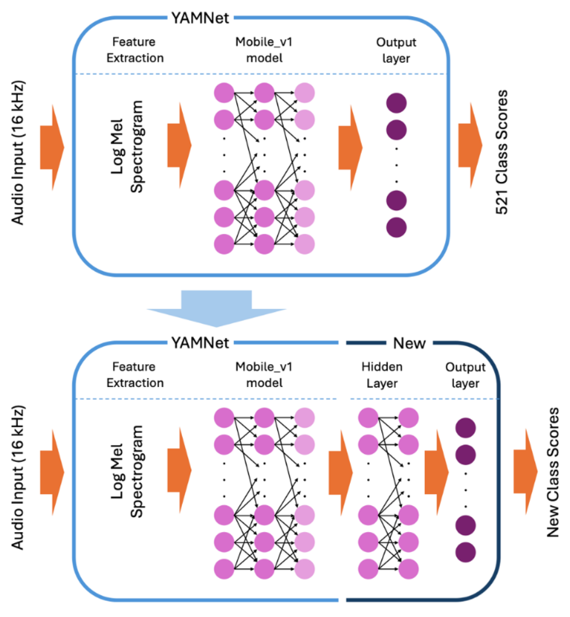
27]. The model can take any length of audio data with a sample rate of 16 kHz. However, the data is split internally into 0.96 second frames with a hop of 0.48 seconds. This is done by taking the full audio data to compute a stabilized log Mel spectrogram with a frequency range of 125 Hz to 7,500 Hz and dividing the results into 0.96 second frames. These frames are then used in the Mobile_v1 model, which produces 1,024 embeddings (the averaged-pooled output of the Mobile_v1 model). These embeddings are fed into a final output layer that produces the 521 audio classes’ scores. For TL, the final output layer is removed, and the embeddings are used to train a new model as seen in
Figure 1.
Ensemble Learning (EL) is a machine learning technique which produces a prediction by utilizing the predictions of multiple trained models. This combined prediction generally performs better than any single model used in the ensemble by compensating for individual models’ biases and by reducing overfitting [
28]. In the context of ESC, since there are numerous types of environmental sounds, it would be beneficial to have multiple “expert” models that are trained on specific signals rather than a single all-encompassing model [
29]. There are multiple ways to implement EL, such as combining the results of multiple similar models trained on different subsets of the data (“bagging”) or training a model on the predictions of different ML models trained on the same data (“stacking”) [
30]. In this study, we trained two different models on the same data and determined the final prediction based on pre-defined criteria that will be discussed later.
2. Data and Methods
2.1. Smartphone High-Explosive Audio Recordings Dataset (SHAReD)
SHAReD consists of 326 multi-sensor smartphone data from 70 surface HE events collected at either Idaho National Laboratory or Nevada National Security Site [
18]. The RedVox application [
31] was used to collect and store the smartphone data, which consisted of data from the microphone, accelerometer, barometer, Global Navigational Satellite System (GNSS) location sensor, and other metadata such as the smartphone model and the sample rate of the sensors. For a more comprehensive description of the RedVox application, we direct the reader to Garcés et al., 2022 [
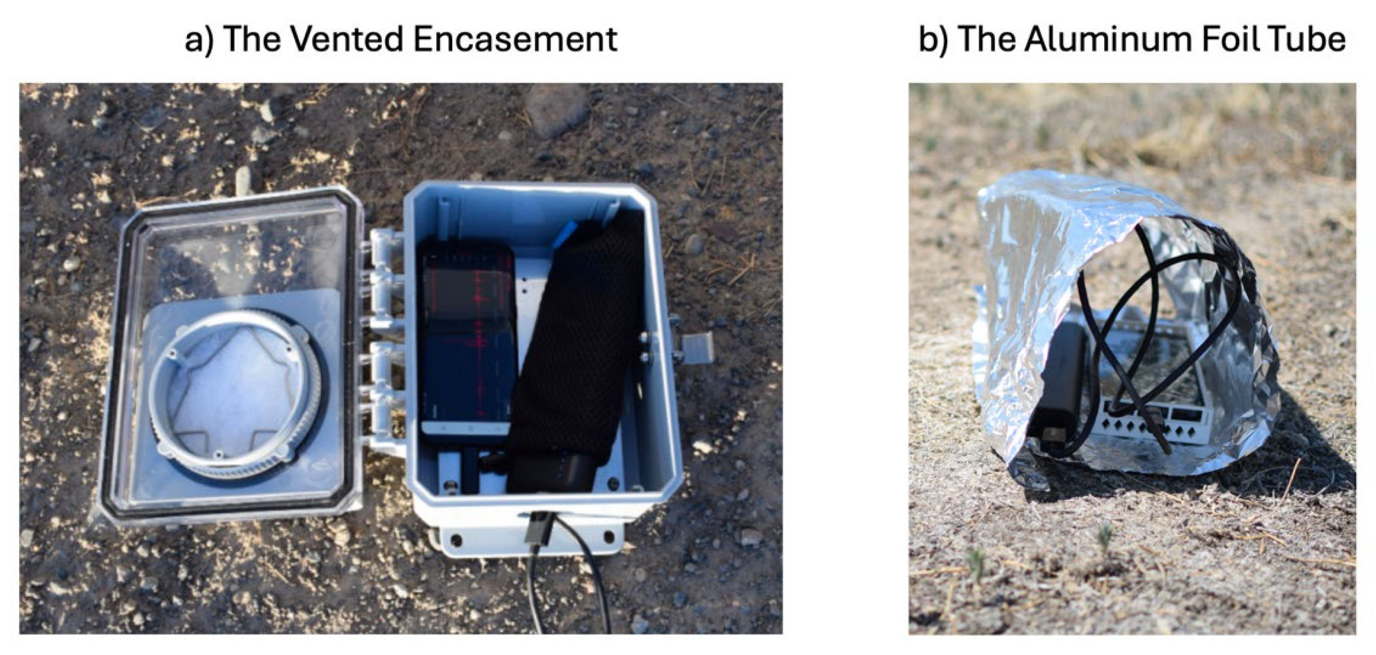
31]. The smartphones were deployed at varying distances near the explosion source in a vented encasement or aluminum foil tube alongside an external battery as shown in
Figure 2. The different deployment configurations were used to protect the smartphones from the elements, specifically direct sunlight, which can cause overheating, or precipitation, which can damage the internal circuitry.
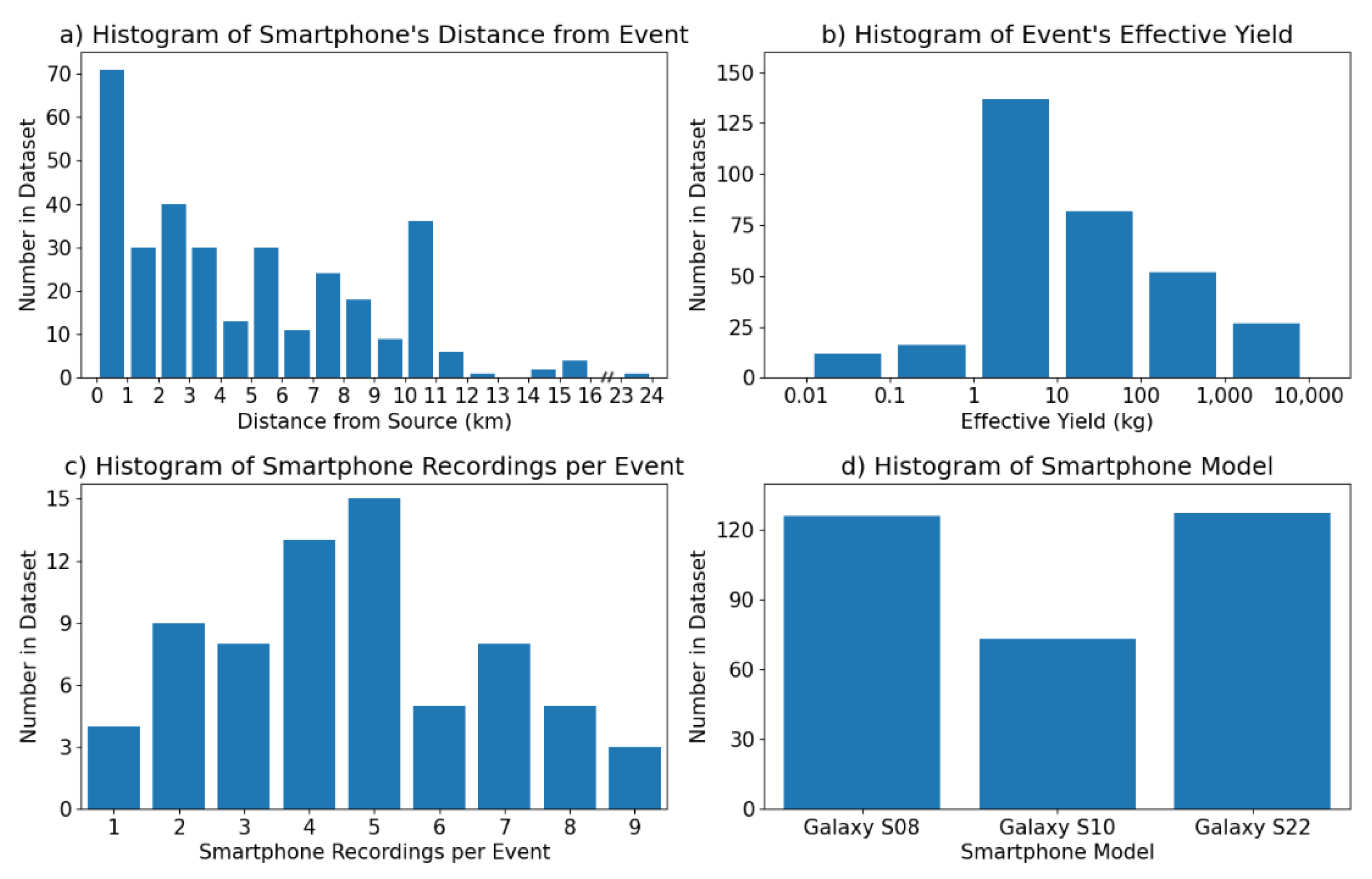
The distances of the smartphones from the explosion source ranged from around 430 m to just over 23 km, but the majority were within 5 km as seen in
Figure 3a. Most of the explosions had effective yields (the amount of TNT required to produce the same amount of energy in free air) between 1 and 100 kg, and the total range spanned from 10 g to 4 tons, as seen in
Figure 3b. Due to differing organizational policies surrounding individual events, the true yield of each explosion may or may not be included in the dataset. However, the effective yield range is included for all events. The histogram of the number of smartphone recordings per event is shown in
Figure 3c. Although there were at least five deployed smartphones for each event, we see that there were a few dozen events with less than five smartphone recordings included in the dataset. This discrepancy is caused by either the yield of the explosion being too small for the signal to travel to all the smartphones or the atmospheric conditions of that day adding significant noise to the signal, as any smartphone recordings with signal-to-noise ratios 3 or less were removed from the dataset. The smartphones used for the dataset were all Samsung Galaxy models, either S8, S10, or S22. The dataset spans multiple years and the smartphones used for the collection were replaced periodically with newer models. The overall distribution of smartphone models represented in the dataset can be seen in
Figure 3d. Further details about the explosion data will be included in a later section.
As previously mentioned, the time-series data included in the dataset are from the microphone, accelerometer, barometer, and the GNSS location sensor. However, the extracted explosion signals from all the sensors were based on the acoustic arrival as the name of the dataset suggests. The duration of the extracted signal is 0.96 seconds and contains the acoustic explosion pulse. Although each set of smartphone data contains a clear explosion signal in the microphone data, depending on the distance of the phone and yield of the explosion, there may not be a visible signal for the accelerometer or barometer data. This was in part due to the higher sensitivity and sample rate of the smartphone microphone sensor. For reference, the sample rate for the microphone was either 800 Hz (63 recordings) or 8,000 Hz (263 recordings), whereas the sample rates for accelerometer averaged around 412 Hz and barometer averaged around 27 Hz. Additionally, 0.96 seconds of “ambient” audio data was included in the dataset by taking microphone data from before or after the explosion. Overall, the smartphone microphones captured a filtered explosion pulse due to their diminishing frequency response in the infrasonic range, however the frequency and time-frequency representations showed great similarities to explosion waveforms captured on infrasound microphones. For those interested in further information on explosion signals captured on smartphone sensors and/or how they compare to infrasound microphones, we direct the reader to Takazawa et al., 2024b [
10], in which a subset of SHAReD is used.
2.2. Training Data
In addition to the explosion and ambient microphone data from the SHAReD, audio from the ESC-50 dataset was also used to train the ML models, as previous work showed improvement from including additional non-explosion data [
32]. The ESC-50 dataset is a collection of 2,000 environmental sound recordings from 50 different classes, and it is often used for benchmarking environmental sound classification [
24,
33,
34]. Some examples of the classes include thunderstorm, fireworks, keyboard typing, clapping, and cow. Each class contains 40 sets of 5 second clips recorded at a sample rate of 44.1 kHz.
Since there were differences in the data (i.e. sample rate, duration), some standardization methods were applied to prepare for machine learning. First, the ESC-50 waveforms were trimmed to a duration of 0.96 seconds to match the waveforms in SHAReD. The trimming was done by taking a randomized segment of the waveform that contained the maximum amplitude. The randomization was added to avoid centering the waveforms on a peak amplitude that could be used as a false feature of ESC-50 waveforms that the ML models could learn. Secondly, the waveforms’ sample rates were adjusted to create two separate datasets with constant sample rates for each of the two ML models. The sample rates were standardized by upsampling or downsampling the waveforms. Thirdly, labels were applied to each category of waveforms (explosion recordings labeled “explosion,” ambient recordings labeled “ambient,” and recordings from ESC-50 labeled “other”). Lastly, the dataset was randomly split into 3 sets: the training set, the validation set, and the test set. Since there was an imbalance in the amount of data (326 each for “explosion” and “ambient”, 2,000 for “other”), the split was applied for each label to ensure a balanced distribution of data (stratified splitting). Additionally, the “explosion” and “ambient” data were split by the explosion event to ensure that the ML models would be robust by testing the model on data from explosions that it has not seen. The distribution of the dataset was roughly 60%, 20%, and 20% for the training, validation, and test sets.
2.3. Machine Learning Models
The first model called Detonation-YAMNet (D-YAMNet), was trained using TL with the YAMNet model. D-YAMNet was constructed by replacing the final output layer of YAMNet with a fully connected layer containing 32 nodes and an output layer with 3 nodes corresponding to “ambient,” “explosion,” and “other.” Sparse categorical cross-entropy was used for the loss function and Adamax [
35] was used for the optimizer, and, in order to further mitigate overfitting, the number of nodes was chosen by iterating through different number of nodes during training and selecting the smallest numbers that kept a minimum of 90% precision for each category. Additionally, class weights were added to address the imbalance in amount of data in the “ambient” and “explosion” categories compared to the “other” category.
The second model was designed to complement the D-YAMNet model by focusing on the lower frequency components of these waveforms, since YAMNet architecture drops all frequency content below 125 Hz. This model will be referred to as the low-frequency model (LFM). To ensure the model concentrated on the low-frequency portion of the input waveform, the sample rate was limited to 800 Hz. Although numerous arguments can be made for different architectures for the LFM, we chose a compact 1D CNN as they are well-suited for real-time and low-cost application (i.e. smartphones) and have shown greater performance on applications that have labeled datasets of limited size [
36]. The LFM consisted of a 1D CNN layer with 16 filters and a kernel size of 11, followed by a 50% dropout layer, a max pooling layer with pool size of 2, a fully connected layer with 32 nodes, and a 3-node output layer. The dropout layer and max pooling layers were added to mitigate overfitting since the LFM is trained on a limited dataset. Additionally, like D-YAMNet, the specifics (number of filters, kernel size, and number of nodes) of the model were determined through iteration and selection of the least complex values that kept a minimum of 90% precision for each category. The same loss function, optimizer, and class weights were used for the training of the LFM as for D-YAMNet.
The ensemble model was constructed using the predictions from the D-YAMNet and LFM with the following criteria: “explosion” if both models predicted “explosion,” “other” if D-YAMNet predicted “other,” and “ambient” for all other cases. For EL using two separate models, stacking is generally used. However, we chose these criteria based on the overall purpose of the ensemble model and insight from the construction of the two incorporated models. The “explosion” prediction was only selected if both models predicted “explosion” to reduce false positive cases, as they can pose an issue for continuous monitoring. The “other” category was solely based on the D-YAMNet prediction since it has the added benefits of TL and covers a wider frequency range that many “other” sound sources would fall under. Although accurately predicting if a non-explosion signal is in the “other” category is not the primary goal for the model, it plays a crucial role in reducing false positive cases for “explosion” as it creates a category for other sounds that a smartphone may pick up while deployed. Overall, these criteria allow the ensemble model to essentially use the LFM to assist D-YAMNet in determining if a waveform classified as “explosion” by the latter should be classified as “explosion” or “ambient.”
3. Results
The models were evaluated using the test set, which was about 20% of the whole dataset and included explosion events that were not included in the training or validation set. The results are showcased using a normalized confusion matrix, where the diagonal represents each category’s true positive rate (recall). The confusion matrix was normalized to clarify results, given the imbalance in the dataset.
3.1. D-YAMNet
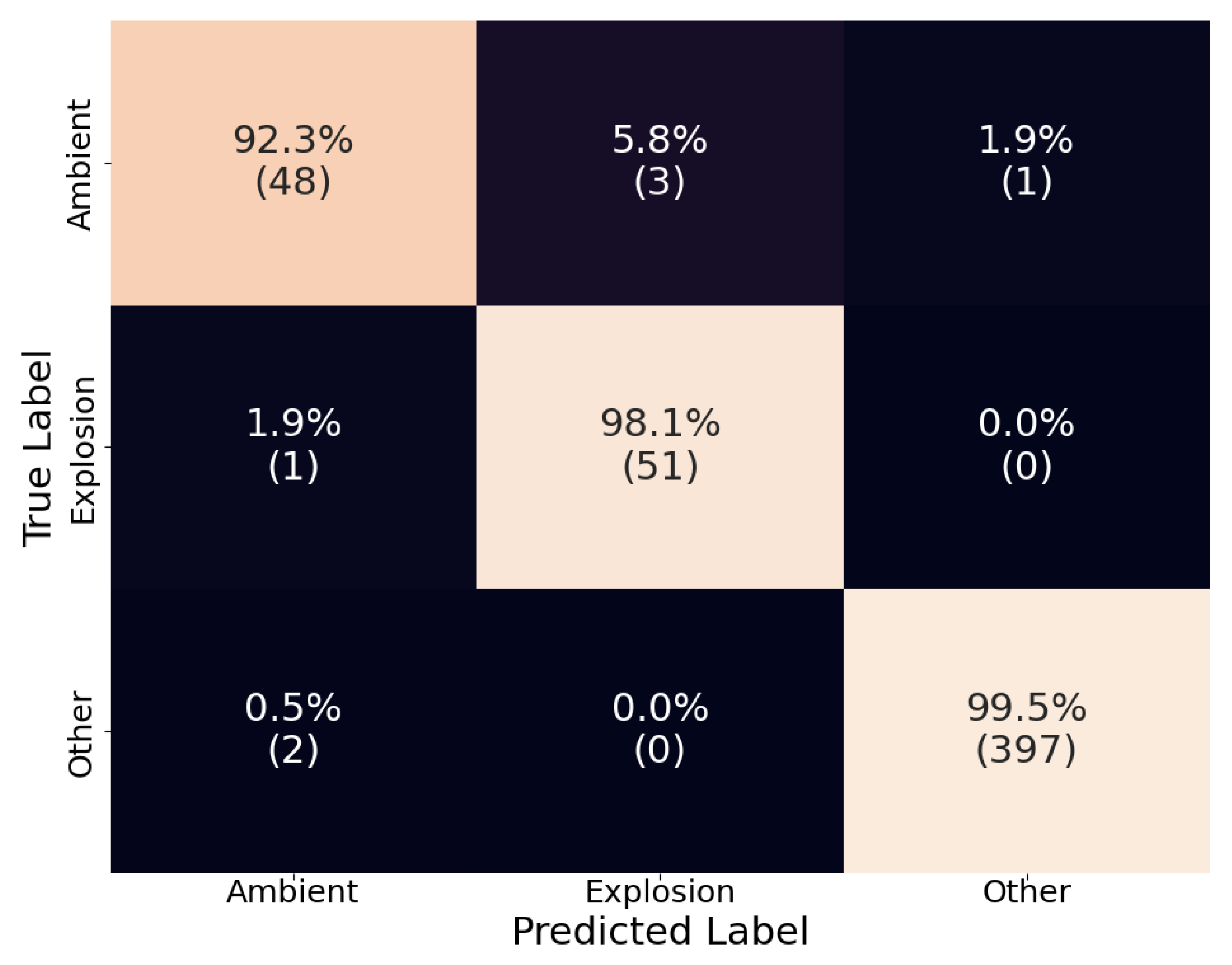
Overall D-YAMNet performed well with each category’s true positive rates of 92.3%, 98.1%, and 99.5% for “ambient,” “explosion,” and “other,” respectively (
Figure 4). The model especially performed well in the “other” category. Although, this model’s purpose is not to identify “other” sound events, this category was added to reduce false positive “explosion” predictions and was successful as there are no false positive cases. In contrast, the model performed worse in the “ambient” category. This relatively low recall of the “ambient” category is most likely due to the nature of the model.
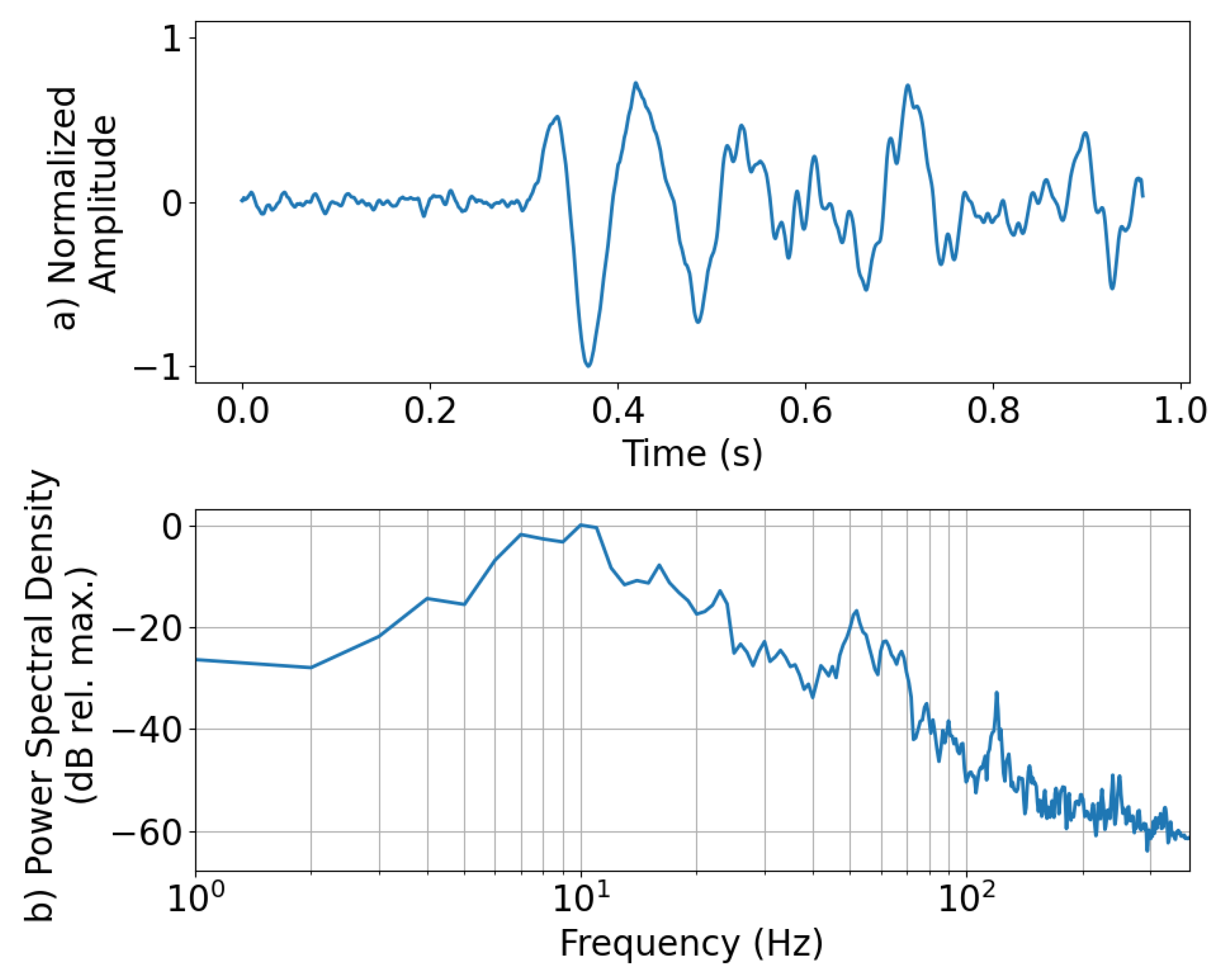
As described earlier, YAMNet ignores frequencies that are below 125 Hz, which is where most of the energy of the explosion signal lies. This could make distinguishing between “explosion” and “ambient” difficult, especially if the waveforms lack significantly identifiable higher-frequency content. To illustrate this, the “explosion” waveform that was falsely categorized as “ambient” is presented along with its power spectral density in
Figure 4.5. This misclassified “explosion” waveform was from an explosion in the 10 kg yield category and recorded on a smartphone roughly 11 km from the source at a sample rate of 800 Hz. For reference, the probability of each class taken from the SoftMax layer of the D-YAMNet was 0.696, 0.304, and 0.000 for “ambient,” “explosion,” and “other,” respectively. From an initial glance at the normalized amplitude (
Figure 5a), we see that the waveform was heavily distorted. Looking at the power spectral density (
Figure 5b), most of the frequency content of the waveform is concentrated below 100 Hz. Additionally, the small frequency spike seen past the 100 Hz mark is located at 120 Hz, which is below the 125 Hz cutoff of the YAMNet model. This majority of the signal’s energy concentration being below the YAMNet’s frequency cutoff, paired with the lack of higher frequency content due to the 800 Hz sample rate of the smartphone microphone, is most likely what led to the model misclassifying the explosion as “ambient.”
3.2. Low-Frequency Model
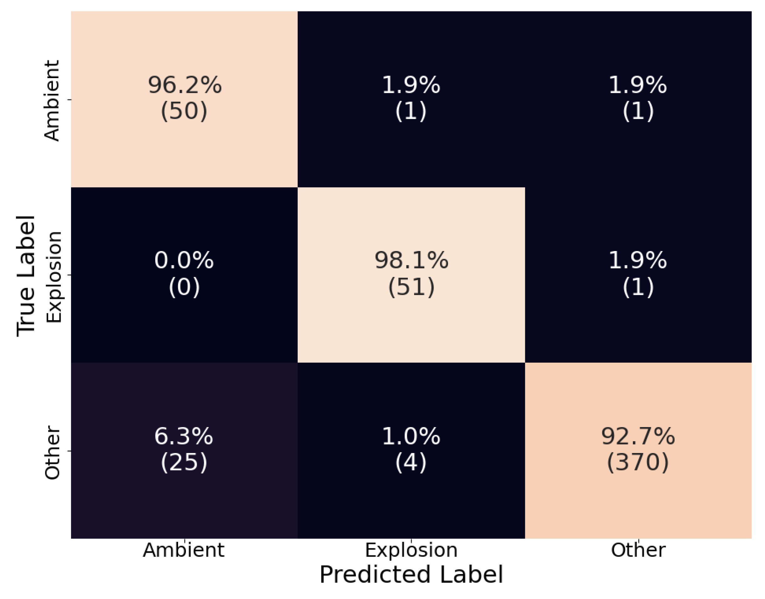
Unlike D-YAMNet, the LFM incorporates all the frequency content of the input data. However, since the waveforms used for training were downsampled to 800 Hz, the model isn’t trained on the higher frequency content of the signals. This resulted in a somewhat reversed outcome compared to D-YAMNet as seen in
Figure 6. Overall, the LFM performed worse than D-YAMNet, which was expected since it was trained on a small dataset without the benefits from transfer learning.
Looking at the recall scores and comparing them to those from D-YAMNet (
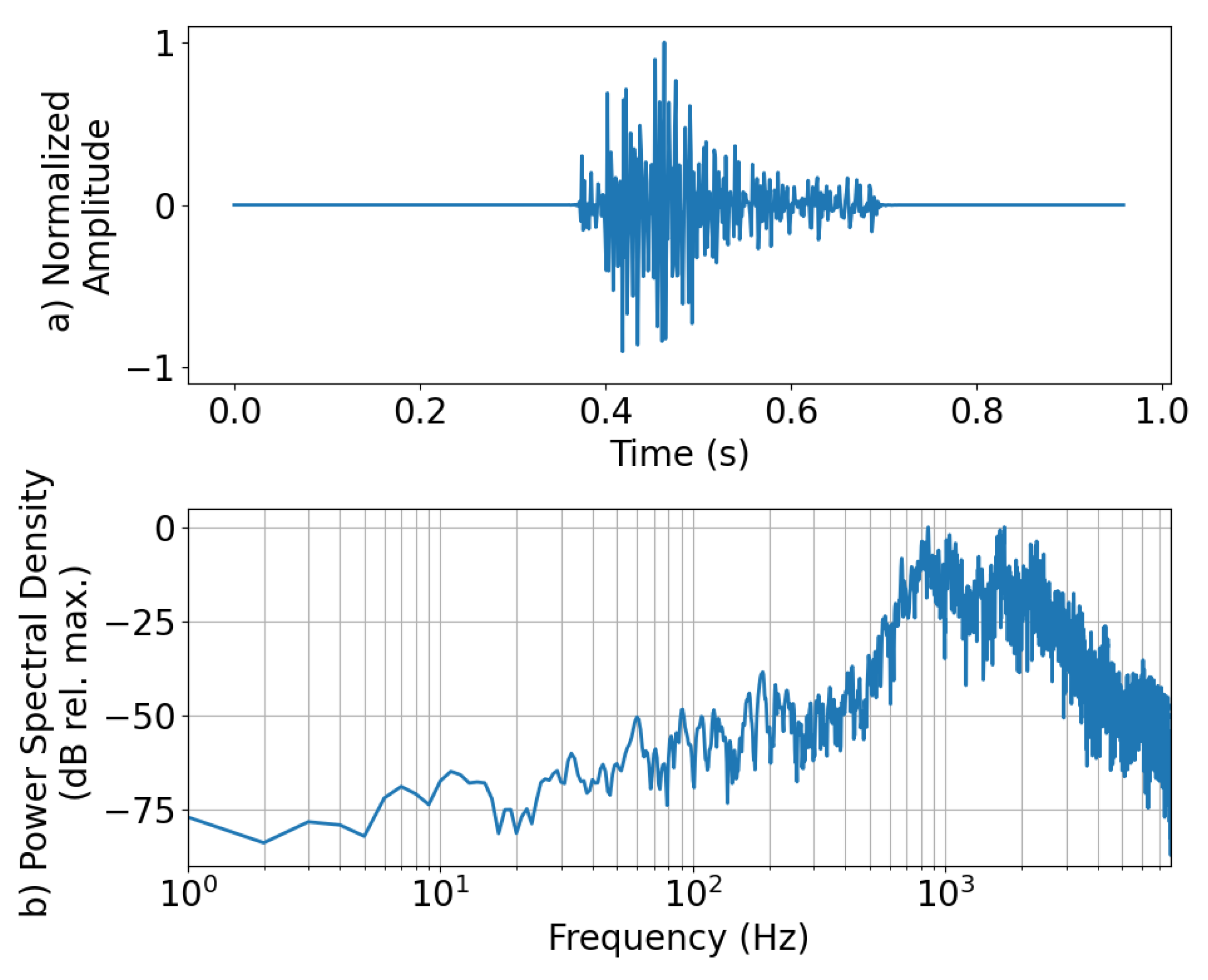
Figure 4), we see that the “ambient” category performed better (96.2%), “explosion” performed the same (98.1%), and the “other” performed worse (92.7%). The relatively high recall scores for the “ambient” and “explosion” classes are likely due to the low-frequency content of the waveforms being kept. However, the worse performance in the “other” category is most likely due to misclassification of those ESC-50 data that mostly contain higher frequency content, which would be removed in the downsampling process making them indistinguishable from “ambient” or “explosion” waveforms. As an example of the latter, a waveform from the “other” category that was misclassified as an “explosion” is presented along with its power spectral density in
Figure 7. This “other” waveform was labeled as “dog” in the ESC-50 dataset. The probabilities for each class taken from the SoftMax layer of the LFM for this waveform were 0.346, 0.514, and 0.140 for “ambient,” “explosion,” and “other,” respectively. Looking at that the normalized amplitude (
Figure 5a), we see that it was a transient sound, however, it does not necessarily resemble an explosion pulse to an experienced eye. Moving to the power spectral density (
Figure 5b), most of the frequency content of the waveform is concentrated above 500 Hz, which is below the 400 Hz cutoff (Nyquist) of the LFM. Additionally, there is a decent amount of energy for frequencies down to 60 Hz. The majority of waveforms’ frequency content being above the cutoff for LFM while also containing some energy in the lower frequencies is most likely what led to the model misclassifying the waveform as “explosion,” although the associated probability was low (0.514).
3.3. Ensemble Model
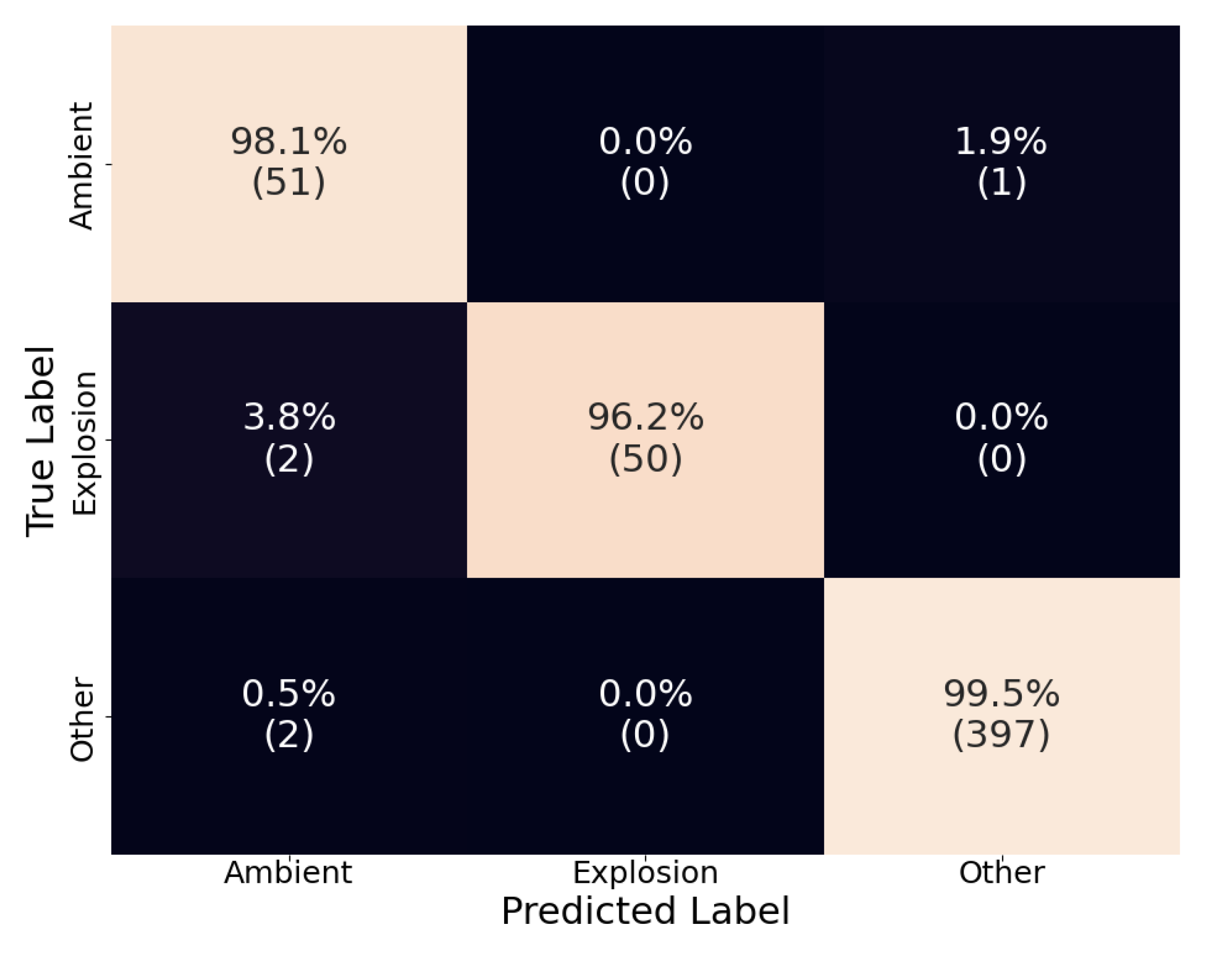
The confusion matrix for the ensemble model can be seen in
Figure 8. Altogether, we see an increased performance with recall above 96% for each category. Only the recall of the “explosion” category saw a slight decrease due to the inclusion of false negatives from both D-YAMNet and LFM. Focusing on the “ambient” and “other” categories, we see that the proposed criteria preserve the high performance of D-YAMNet in the “other” category while, simultaneously, the addition of the LFM improves the results in the “ambient” category. More importantly, we see that the ensemble model was able to eliminate false positives in the “explosion” category entirely, which translates to a much more stable and robust model that can be used for real-time explosion monitoring.
4. Discussion and Conclusion
Two ML models (D-YAMNet and LFM) were trained and tested using two datasets (SHAReD and ESC-50) and then combined into an ensemble model for explosion detection using smartphones. Although both D-YAMNet and LFM had recall scores over 90% for each category, each model had a weak point in one category: “ambient” for D-YAMNet and “other” for LFM. These shortcomings were explained by the construction of the models. For D-YAMNet, the low-frequency information (<125 Hz) of the waveforms was not incorporated, which would make it difficult to distinguish “ambient” sounds (which were mostly silent) from “explosion” sounds that have the majority of their energy concentrated in the lower frequencies. For LFM, the sample rate of the input data was limited to 800 Hz, which made “other” sounds with primarily high frequency information harder to distinguish from “ambient” sounds. The ensemble model was able to compensate for each model’s shortcomings, which resulted in a combined model that performed better overall, with >96% recall in each category. Additionally, the ensemble model eliminated all false positive cases in the “explosion” category, creating a robust model for explosion monitoring.
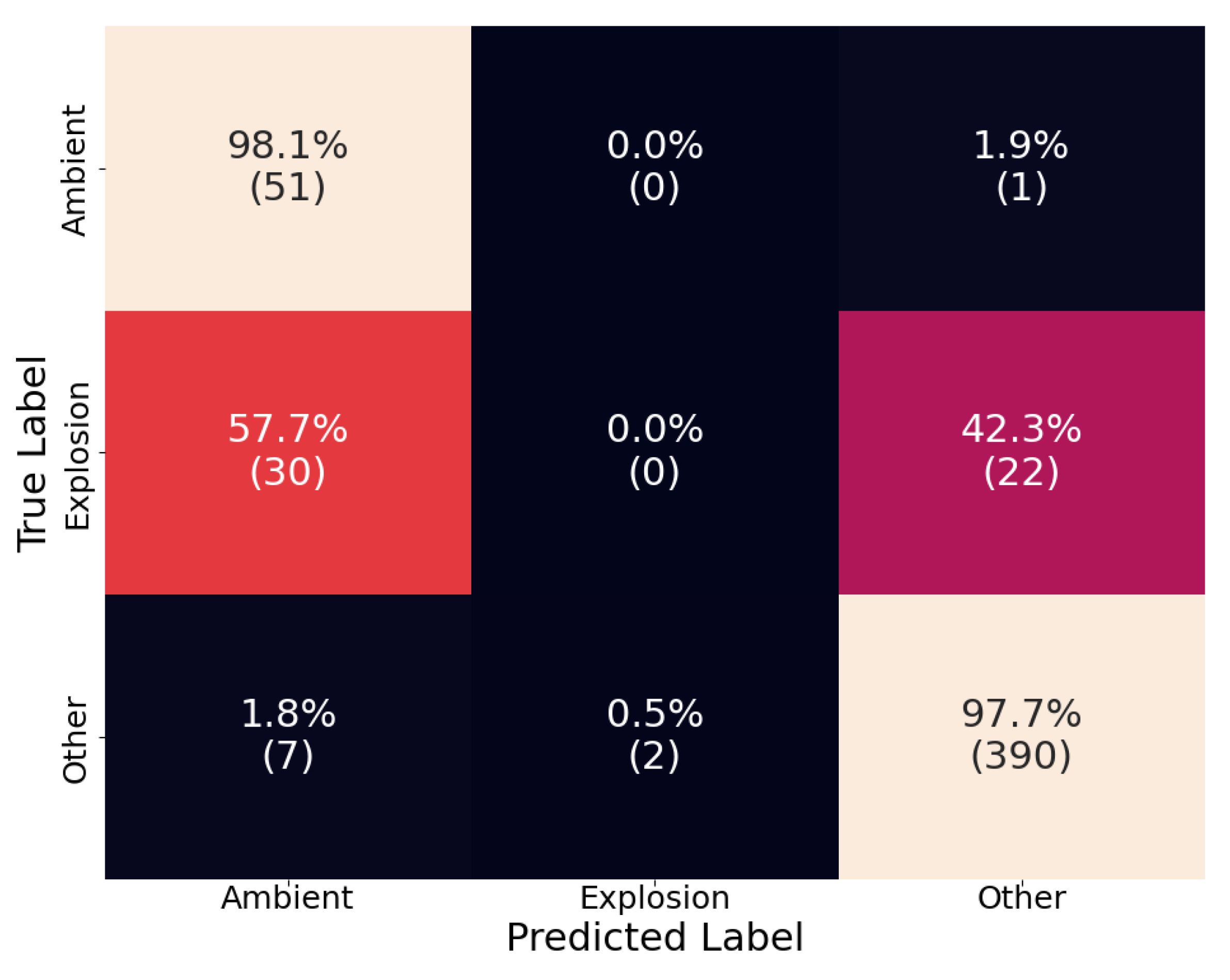
Since explosion detection on smartphone sensors using machine learning is a relatively new endeavor, there are no specialized explosion detection models that can be used as a baseline comparison to evaluate the ensemble model’s performance. However, the base YAMNet model does include an “explosion” class that can be used for a comparison. We used the test dataset to evaluate the performance of YAMNet by mapping the 521 classes to the following: “explosion” if YAMNet predicted “explosion,” “ambient” if YAMNet predicted “silence,” and “other” for all other classes. The resulting confusion matrix is shown in
Figure 9. We see that YAMNet performed well at classifying “ambient” and “other” sounds, with 98.1% and 97.7% recall, respectively. However, it was not able to correctly classify a single explosion properly. More interestingly it seems to have categorized roughly half of the “explosion” sounds as “ambient” and half as “other.” This poor performance of the base YAMNet model is most likely due to the training data, which mostly consists of “explosion sounds” from video games and movies, as well as gunshots which aren’t HEs.
Although the initial success of the ensemble model is promising, it is still based on a limited dataset (<3000 waveforms). Continued efforts in explosion data collection and public release of such data will be essential for improving the performance of explosion detection models. Future work should include deploying smartphones to test the ensemble model in deployments for real-time detection. Additionally, developing algorithms to take into account the explosion detection results from all nearby smartphones should improve reliability. The results of the ensemble model presented in this work indicate that, with more data to train models on, rigorous testing in the field, and effective integration of predictions from multiple models and devices, smartphones will prove to be a viable ubiquitous sensor network for explosion detection and a valuable addition to the arsenal of explosion monitoring methods.
Author Contributions
Conceptualization, S.K.T. and M.A.G.; methodology, S.K.T.; software, S.K.T., S.K.P., and M.A.G.; validation, S.K.T., S.K.P., L.A.O., C.P.Z. and M.A.G.; formal analysis, S.K.T; investigation, S.K.T., S.K.P., L.A.O., J.D.H, S.J.T, and C.P.Z.; resources, L.A.O., J.D.H, S.J.T, D.L.C, C.P.Z., and M.A.G.; data curation, S.K.T; writing—original draft preparation, S.K.T, S.K.P., and M.A.G.; writing—review and editing, (TO BE ADDED) ; visualization, S.K.T.; supervision, L.A.O., D.L.C., C.P.Z., and M.A.G.; project administration, M.A.G.; funding acquisition, M.A.G. All authors have read and agreed to the published version of the manuscript
Funding
This work was supported by the Department of Energy National Nuclear Security Administration under Award Numbers DE-NA0003920 (MTV) and DE-NA0003921 (ETI).
Data Availability Statement
The data (SHAReD [
18]) used for this research is available as a pandas DataFrame [
37] along with D-YAMNet and LFM. The data and models can be found in the Harvard Dataverse open-access repository with the following Digital Object Identifier doi: 10.7910/DVN/ROWODP.
Acknowledgments
The authors are thankful to contributions from J. Tobin while he was a graduate student at ISLA. We are also grateful to assoc. prof. J. H. Lee for providing review and expert advice, and to anonymous reviewers who helped improve the manuscript.
Conflicts of Interest
The authors declare no conflicts of interest. The funders had no role in the design of the study; in the collection, analyses, or interpretation of data; in the writing of the manuscript, or in the decision to publish the results.
References
- Garces, M.A. Explosion Source Models. In: Le Pichon, A., Blanc, E., Hauchecorne, A. (Eds.), Infrasound Monitoring for Atmospheric Studies; 2019; ISBN 9781402095078.
- Vergoz, J.; Hupe, P.; Listowski, C.; Le Pichon, A.; Garcés, M.A.; Marchetti, E.; Labazuy, P.; Ceranna, L.; Pilger, C.; Gaebler, P.; et al. IMS Observations of Infrasound and Acoustic-Gravity Waves Produced by the January 2022 Volcanic Eruption of Hunga, Tonga: A Global Analysis. Earth Planet Sci Lett 2022, 591, 117639. [CrossRef]
- Ceranna, L.; Le Pichon, A.; Green, D.N.; Mialle, P. The Buncefield Explosion: A Benchmark for Infrasound Analysis across Central Europe. Geophys J Int 2009, 177, 491–508. [CrossRef]
- Gitterman, Y. SAYARIM INFRASOUND CALIBRATION EXPLOSION: NEAR-SOURCE AND LOCAL OBSERVATIONS AND YIELD ESTIMATION; 2010;
- Fuchs, F.; Schneider, F.M.; Kolínský, P.; Serafin, S.; Bokelmann, G. Rich Observations of Local and Regional Infrasound Phases Made by the AlpArray Seismic Network after Refinery Explosion. Sci Rep 2019, 9, 1–14. [CrossRef]
- Fee, D.; Toney, L.; Kim, K.; Sanderson, R.W.; Iezzi, A.M.; Matoza, R.S.; Angelis, S. De; Jolly, A.D.; Lyons, J.J.; Haney, M.M.; et al. Local Explosion Detection and Infrasound Localization by Reverse Time Migration Using 3-D Finite-Difference Wave Propagation. 2021, 9, 1–14. [CrossRef]
- Blom, P. Regional Infrasonic Observations from Surface Explosions-Influence of Atmospheric Variations and Realistic Terrain. Geophys J Int 2023, 235, 200–215. [CrossRef]
- Kim, K.; Pasyanos, M.E. Seismoacoustic Explosion Yield and Depth Estimation: Insights from the Large Surface Explosion Coupling Experiment. Bulletin of the Seismological Society of America 2023, 113, 1457–1470. [CrossRef]
- Chen, T.; Larmat, C.; Blom, P.; Zeiler, C. Seismoacoustic Analysis of the Large Surface Explosion Coupling Experiment Using a Large-N Seismic Array. Bulletin of the Seismological Society of America 2023, 113, 1692–1701. [CrossRef]
- Takazawa, S.K.; Popenhagen, S.; Ocampo Giraldo, L.; Cardenas, E.; Hix, J.; Thompson, S.; Chichester, D.; Garces, M.A. A Comparison of Smartphone and Infrasound Microphone Data from a Fuel Air Explosive and a High Explosive. J Acoust Soc Am.
- Lane, N.D.; Miluzzo, E.; Lu, H.; Peebles, D.; Choudhury, T.; Campbell, A.T. A Survey of Mobile Phone Sensing. IEEE Communications Magazine 2010, 48, 140–150. [CrossRef]
- Ganti, R.K.; Ye, F.; Lei, H. Mobile Crowdsensing: Current State and Future Challenges. IEEE Communications Magazine 2011, 49, 32–39. [CrossRef]
- Capponi, A.; Fiandrino, C.; Kantarci, B.; Foschini, L.; Kliazovich, D.; Bouvry, P. A Survey on Mobile Crowdsensing Systems: Challenges, Solutions, and Opportunities. IEEE Communications Surveys and Tutorials 2019, 21, 2419–2465. [CrossRef]
- Thandu, S.C.; Chellappan, S.; Yin, Z. Ranging Explosion Events Using Smartphones. 2015 IEEE 11th International Conference on Wireless and Mobile Computing, Networking and Communications, WiMob 2015 2015, 492–499. [CrossRef]
- Mahapatra, C.; Mohanty, A.R. Explosive Sound Source Localization in Indoor and Outdoor Environments Using Modified Levenberg Marquardt Algorithm. Measurement (Lond) 2022, 187, 110362. [CrossRef]
- Mahapatra, C.; Mohanty, A.R. Optimization of Number of Microphones and Microphone Spacing Using Time Delay Based Multilateration Approach for Explosive Sound Source Localization. Applied Acoustics 2022, 198, 108998. [CrossRef]
- Popenhagen, S.K.; Bowman, D.C.; Zeiler, C.; Garcés, M.A. Acoustic Waves From a Distant Explosion Recorded on a Continuously Ascending Balloon in the Middle Stratosphere. Geophys Res Lett 2023, 50. [CrossRef]
- Takazawa, S.K. Smartphone High-Explosive Audio Recordings Dataset (SHAReD) Available online: https://dataverse.harvard.edu/dataset.xhtml?persistentId=doi:10.7910/DVN/ROWODP (accessed on 11 June 2024).
- Piczak, K.J. ESC: Dataset for Environmental Sound Classification. MM 2015 - Proceedings of the 2015 ACM Multimedia Conference 2015, 1015–1018. [CrossRef]
- Plakal, M.; Ellis, D. YAMNet 2019.
- Pan, S.J.; Yang, Q. A Survey on Transfer Learning. IEEE Trans Knowl Data Eng 2010, 22, 1345–1359. [CrossRef]
- Brusa, E.; Delprete, C.; Di Maggio, L.G. Deep Transfer Learning for Machine Diagnosis: From Sound and Music Recognition to Bearing Fault Detection. Applied Sciences (Switzerland) 2021, 11. [CrossRef]
- Tsalera, E.; Papadakis, A.; Samarakou, M. Comparison of Pre-Trained Cnns for Audio Classification Using Transfer Learning. Journal of Sensor and Actuator Networks 2021, 10. [CrossRef]
- Ashurov, A.; Zhou, Y.; Shi, L.; Zhao, Y.; Liu, H. Environmental Sound Classification Based on Transfer-Learning Techniques with Multiple Optimizers. Electronics (Switzerland) 2022, 11, 1–20. [CrossRef]
- Hyun, S.H. Sound-Event Detection of Water-Usage Activities Using Transfer Learning. Sensors 2023, 24, 22. [CrossRef]
- Gemmeke, J.F.; Ellis, D.P.W.; Freedman, D.; Jansen, A.; Lawrence, W.; Moore, R.C.; Plakal, M.; Ritter, M. Audio Set: An Ontology and Human-Labeled Dataset for Audio Events,In Proceedings of IEEE International Conference on Acoustics, Speech and Signal Processing (ICASSP), New Orleans, LA, USA, 2017, Pp. 776-780. [CrossRef]
- Howard, A.G.; Zhu, M.; Chen, B.; Kalenichenko, D.; Wang, W.; Weyand, T.; Andreetto, M.; Adam, H. MobileNets: Efficient Convolutional Neural Networks for Mobile Vision Applications. 2017.
- Sagi, O.; Rokach, L. Ensemble Learning: A Survey. Wiley Interdiscip Rev Data Min Knowl Discov 2018, 8, 1–18. [CrossRef]
- Chachada, S.; Kuo, C.C.J. Environmental Sound Recognition: A Survey. 2013 Asia-Pacific Signal and Information Processing Association Annual Summit and Conference, APSIPA 2013 2013. [CrossRef]
- Hastie, T.; Tibshirani, R.; Friedman, J. The Elements of Statistical Learning; Springer Series in Statistics; Springer New York: New York, NY, 2009; ISBN 978-0-387-84857-0.
- Garcés, M.; Bowman, D.; Zeiler, C.; Christe, A.; Yoshiyama, T.; Williams, B.; Colet, M.; Takazawa, S.; Popenhagen, S.; Hatanaka, Y.; et al. Skyfall 2020: Smartphone Data from a 36 Km Drop. 2021, 1–23.
- Takazawa, S.K.; Garces, M.A.; Ocampo Giraldo, L.; Hix, J.; Chichester, D.; Zeiler, C. Explosion Detection with Transfer Learning via YAMNet and the ESC-50 Dataset. In Proceedings of the University Program Review (UPR) 2022 Meeting for Defense Nuclear Nonproliferation Research and Development Program; 2022.
- Piczak, K.J. Environmental Sound Classification with Convolutional Neural Networks. In Proceedings of the IEEE International Workshop on Machine Learning for Signal Processing, MLSP; 2015.
- Huzaifah, M. Comparison of Time-Frequency Representations for Environmental Sound Classification Using Convolutional Neural Networks. 2017, 1–5.
- Kingma, D.P.; Ba, J.L. Adam: A Method for Stochastic Optimization. 3rd International Conference on Learning Representations, ICLR 2015 - Conference Track Proceedings 2015, 1–15.
- Kiranyaz, S.; Avci, O.; Abdeljaber, O.; Ince, T.; Gabbouj, M.; Inman, D.J. 1D Convolutional Neural Networks and Applications: A Survey. Mech Syst Signal Process 2021, 151, 107398. [CrossRef]
- The pandas development team Pandas-Dev/Pandas: Pandas 2024.
|
Disclaimer/Publisher’s Note: The statements, opinions and data contained in all publications are solely those of the individual author(s) and contributor(s) and not of MDPI and/or the editor(s). MDPI and/or the editor(s) disclaim responsibility for any injury to people or property resulting from any ideas, methods, instructions or products referred to in the content. |
© 2024 by the authors. Licensee MDPI, Basel, Switzerland. This article is an open access article distributed under the terms and conditions of the Creative Commons Attribution (CC BY) license (http://creativecommons.org/licenses/by/4.0/).
