Submitted:
25 July 2024
Posted:
26 July 2024
You are already at the latest version
Abstract
Keywords:
1. Introduction
2. Materials and Methods
2.1. Waveform Generation
2.2. Square Wave
2.3. Triangular Wave
2.4. Sine Wave
2.5. CNN
3. Real-World Noisy Signal
4. Discussion
Conflicts of Interest
References
- Goodfellow, I.; Bengio, Y.; Courville, A. Deep Learning, 1st ed.; MIT Press: Cambridge, USA, 2016; pp. 499–500. [Google Scholar]
- Leite, N. M. N.; Pereira, E. T.; Gurjão, E. C.; Veloso, L. R. Deep Convolutional Autoencoder for EEG Noise Filtering. In Proceedings of the IEEE International Conference on Bioinformatics and Biomedicine (BIBM), Madrid, Spain, 03-06 December 2018. [Google Scholar]
- Fuchs, J.; Dubey, A.; Lübke, M.; Weigel, R.; Lurz F., E. F. In The Automotive Radar Interference Mitigation using a Convolutional Autoencoder. In Proceedings of the IEEE International Radar Conference (RADAR), Washington DC, US, 28-30 April 2020. [Google Scholar]
- Yasenko, L.; Klyatchenko, Y.; Tarasenko-Klyatchenko, O. Image noise reduction by denoising autoencoder. Proceedings of 11th IEEE International Conference on Dependable Systems, Services and Technologies, DESSERT’2020, Kyiv, Ukraine, 14-18 May 2020. [Google Scholar]
- Gao, F.; Li, B.; Chen, L.; Wei, X.; Shang, Z.; He, C. Ultrasonic signal denoising based on autoencoder. Review of Scientific Instruments 2020, 91, 1–9. [Google Scholar] [CrossRef] [PubMed]
- Saad, O. M.; Chen, Y. Deep denoising autoencoder for seismic random noise attenuation. Geophysics 2020, 85, 367–376. [Google Scholar] [CrossRef]
- Yu, J.; Zhou, X. One-Dimensional Residual Convolutional Autoencoder Based Feature Learning for Gearbox Fault Diagnosis. IEEE Transactions on Industrial Informatics 2020, 16, 6347–6358. [Google Scholar] [CrossRef]
- Liu, X.; Zhou, Q.; Zhao, J.; Shen, H.; Xiong, X. Fault Diagnosis of Rotating Machinery under Noisy Environment Conditions Based on a 1-D Convolutional Autoencoder and 1-D Convolutional Neural Network. Sensors 2019, 19, 1–20. [Google Scholar] [CrossRef] [PubMed]
- Sheu, M. H.; Jhang, Y. S.; Chang, Y. C.; Wang, S. T.; Chang, C. Y.; Lai, S. C. Lightweight Denoising Autoencoder Design for Noise Removal in Electrocardiography. IEEE Access 2022, 10, 98104–98116. [Google Scholar] [CrossRef]
- Zhang, M.; Diao, M.; Guo, L. Convolutional Neural Networks for Automatic Cognitive Radio Waveform Recognition. IEEE Access 2017, 5, 11074–11082. [Google Scholar] [CrossRef]
- Kim, J.; Ko, J.; Choi, H.; Kim, H. Printed Circuit Board Defect Detection Using Deep Learning via a Skip-Connected Convolutional Autoencoder. Sensors 2021, 21, 1–13. [Google Scholar] [CrossRef] [PubMed]
- Xu, X.; Feng, J.; Zhan, L.; Li, Z.; Qian, F.; Yan, Y. Fault Diagnosis of Permanent Magnet Synchronous Motor Based on Stacked Denoising Autoencoder. Entropy 2021, 23, 1–13. [Google Scholar] [CrossRef] [PubMed]
- Xiao, J.; Ma, W.; Lou, J.; Jiang, J.; Huang, Y.; Shi, Z.; Shen, Q.; Yang, X. Circuit reliability prediction based on deep autoencoder network. Neurocomputing 2019, 370, 140–154. [Google Scholar] [CrossRef]
- Kong, S. H.; Kim, M.; Zhan, L; Hoang, Z.M. Automatic LPI Radar Waveform Recognition using CNN. IEEE Access 2018, 6, 4207–4219. [Google Scholar] [CrossRef]
- Si, W.; Wan, C.; Zhang, C. Towards an accurate radar waveform recognition algorithm based on dense CNN. Multimedia Tools and Applications 2021, 80, 1179–1192. [Google Scholar] [CrossRef]
- Qu, Z.; Wang, W.; Hou; Hou, C. Radar Signal Intra-Pulse Modulation Recognition Based on Convolutional Denoising Autoencoder and Deep Convolutional Neural Network. IEEE Access 2019, 7, 112339–112347. [Google Scholar] [CrossRef]
- Taswell, C. The what, how, and why of wavelet shrinkage denoising. Computing in Science and Engineering 2000, 2, 12–19. [Google Scholar] [CrossRef]
- Gomez, J. L.; Velis, D. R. A simple method inspired by empirical mode decomposition for denoising seismic data. Geophysics 2016, 81, 403–413. [Google Scholar] [CrossRef]
- Moore, R.; Ezekiel, S.; Blasch, E. Denoising one-dimensional signals with curvelets and contourlets. Proceedings of NAECON 2014 - IEEE National Aerospace and Electronics Conference, Dayton, US, 24-27 June 2014. [Google Scholar]
- Green, L. Understanding the importance of signal integrity. IEEE Circuits and Devices Magazine 1999, 15, 7–10. [Google Scholar] [CrossRef]
- Sewak, M.; Karim, M. R.; Pujari, P. Practical Convolutional Networks, 1st. ed.; Publisher: Packt Birmingham, UK, 2018; pp. 1–211. [Google Scholar]
- Abdipour, A.; Moradi, G.; Saboktakin, S. Design and implementation of a noise generator. In Proceedings of the IEEE International RF and Microwave Conference, Kuala Lampur, Malaysia, 02-04 December 2008. [Google Scholar]
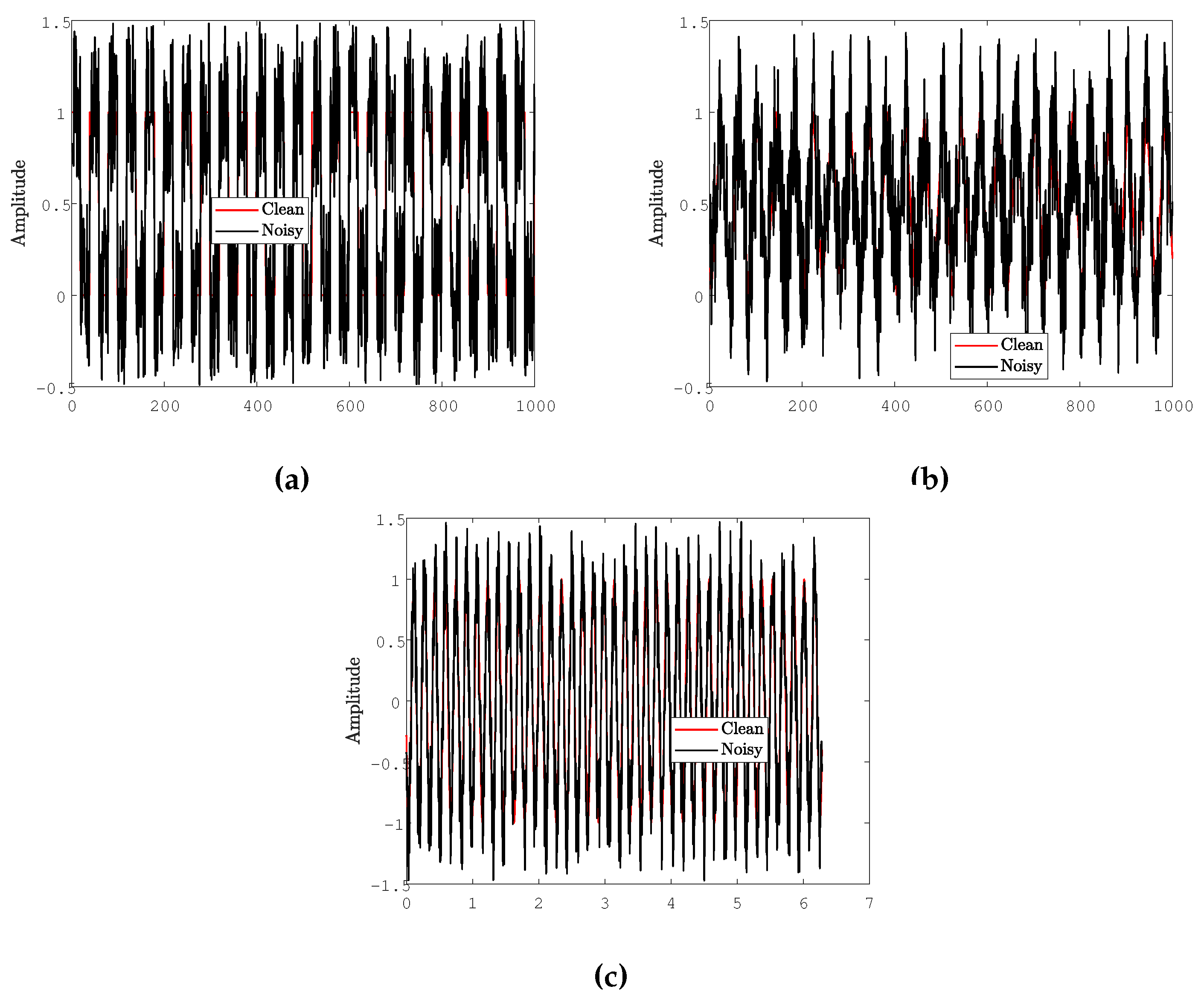
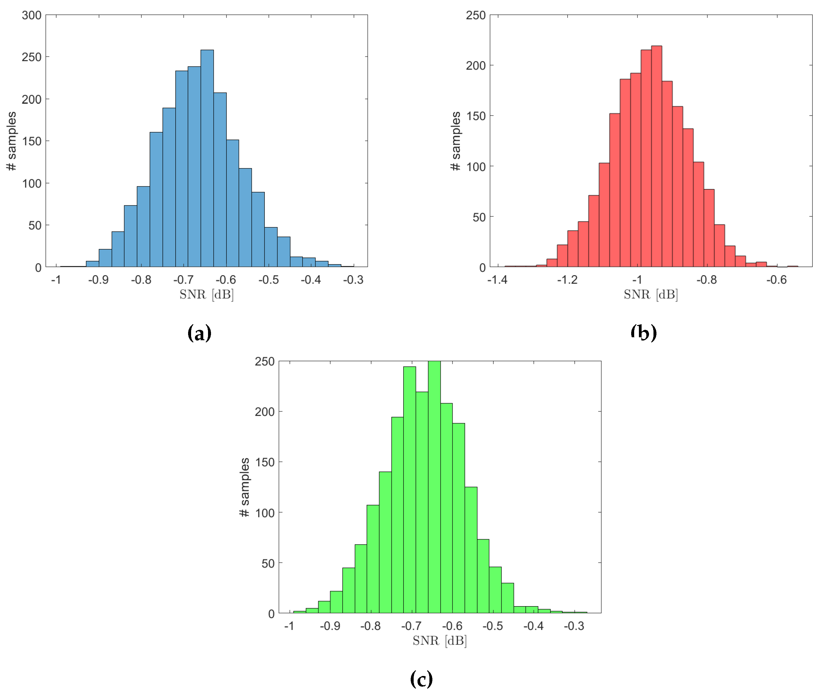
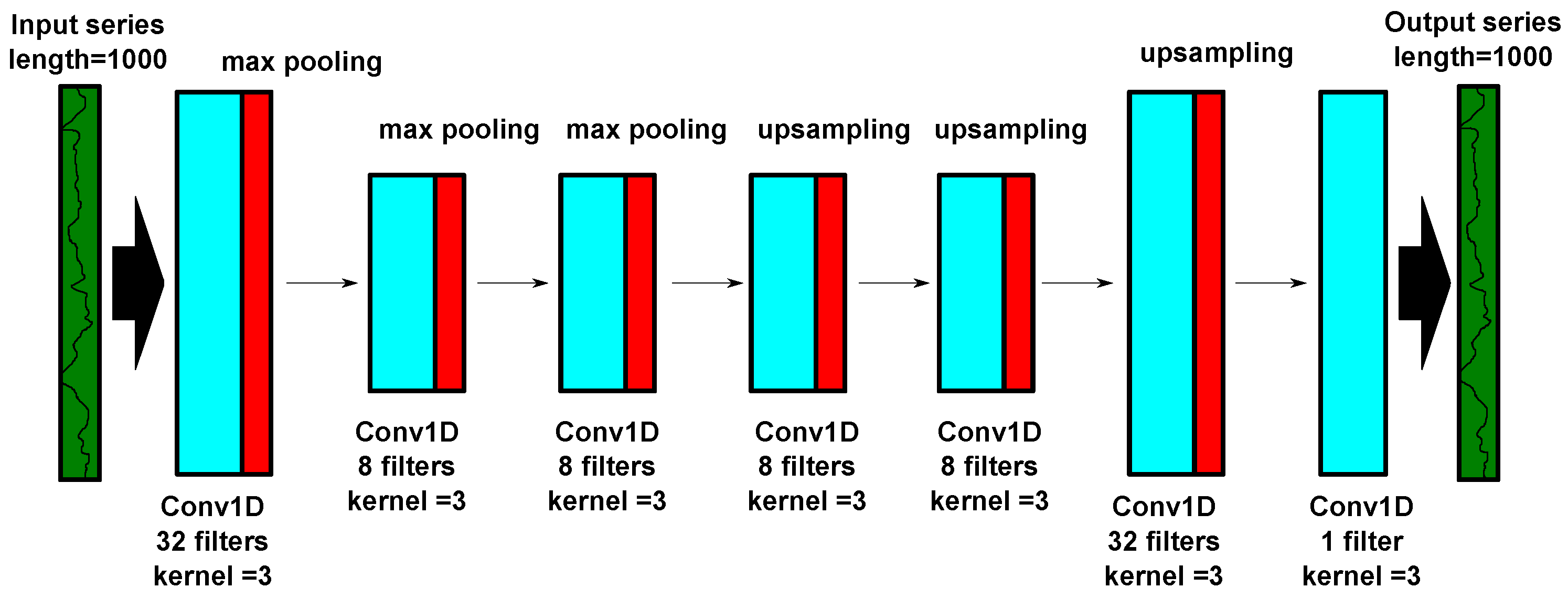
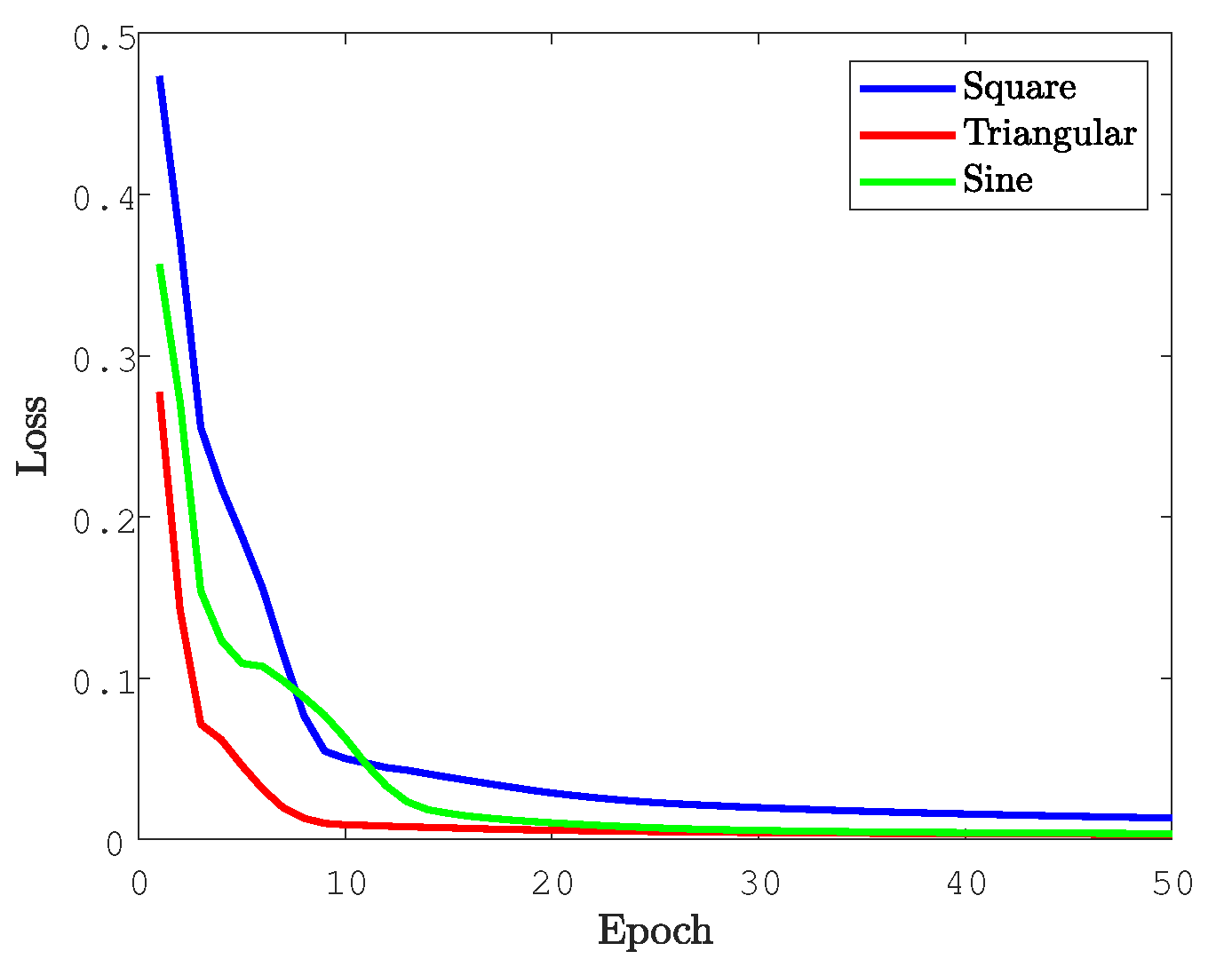
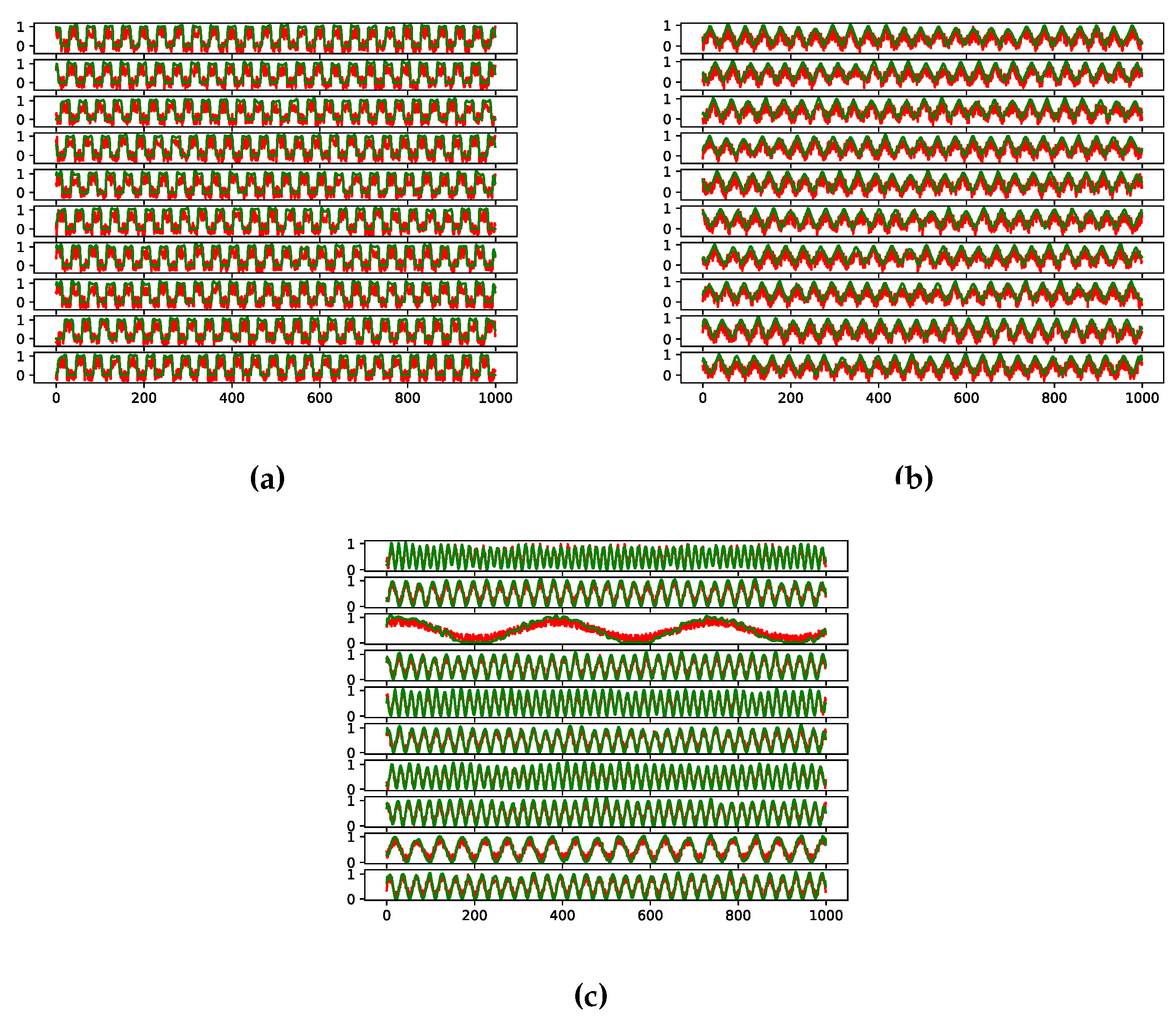
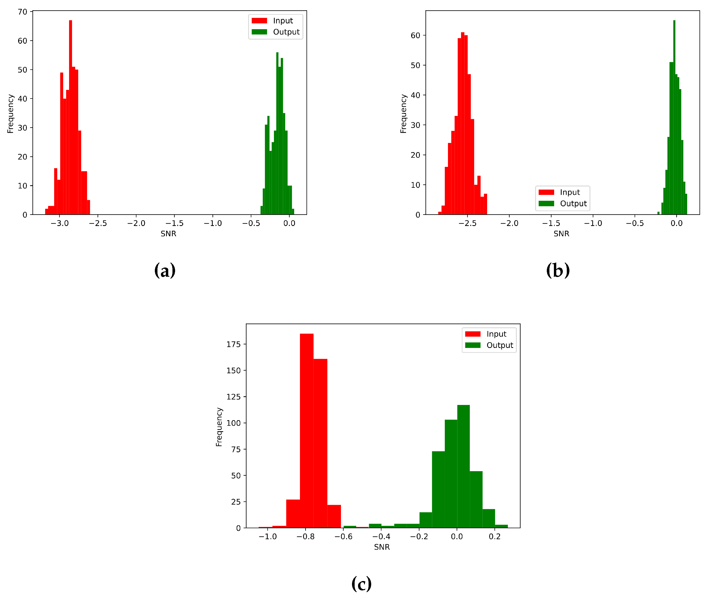
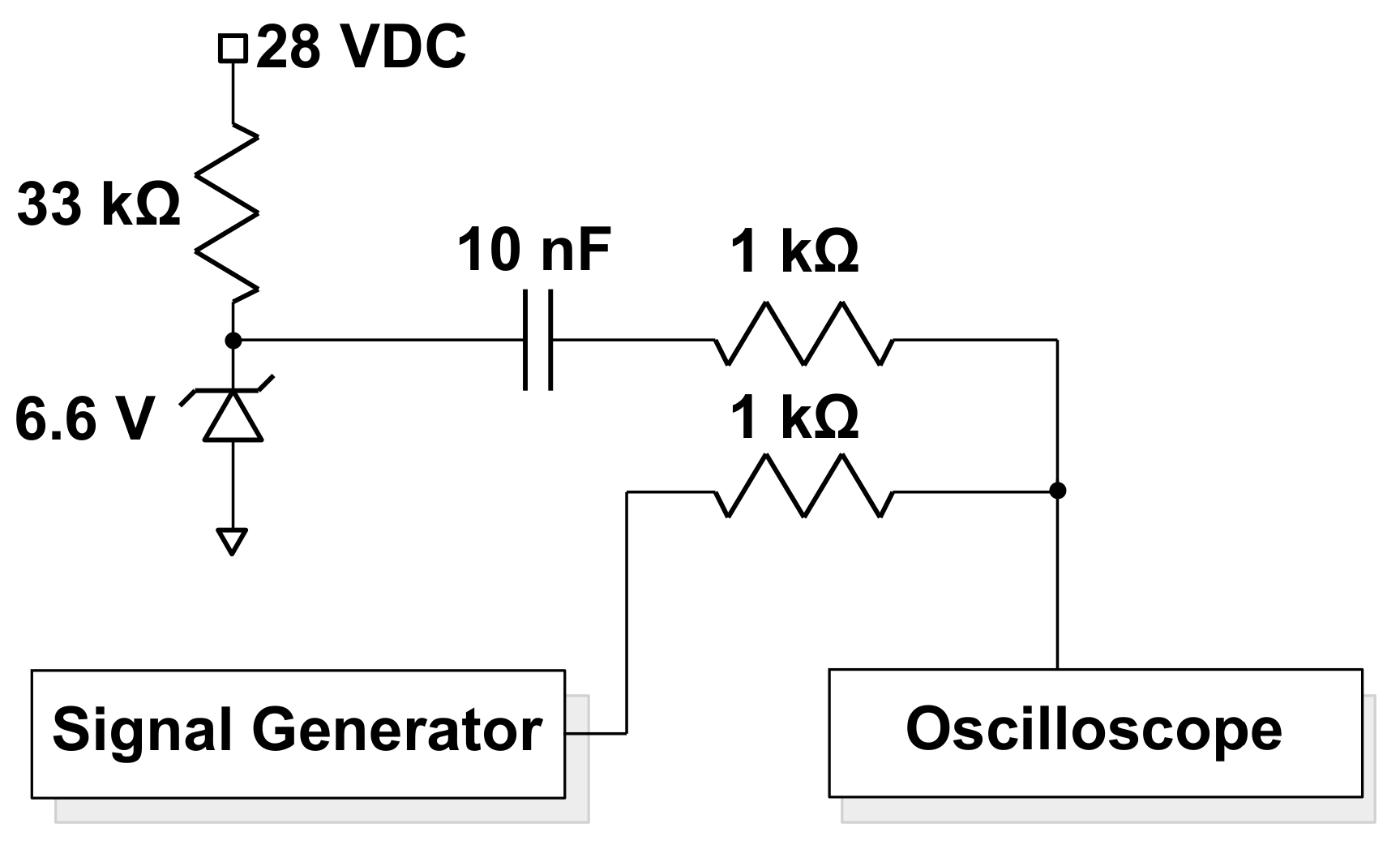
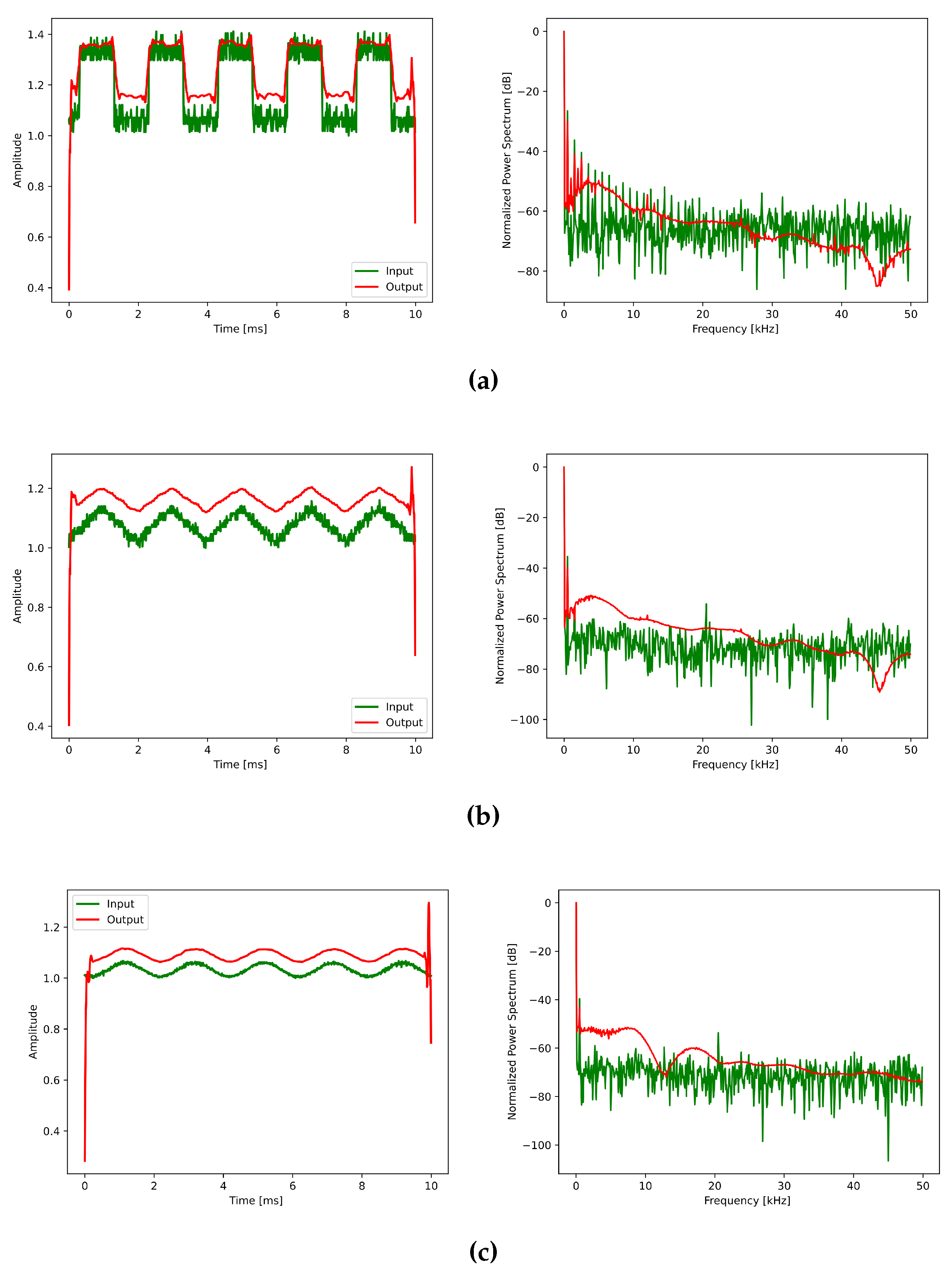
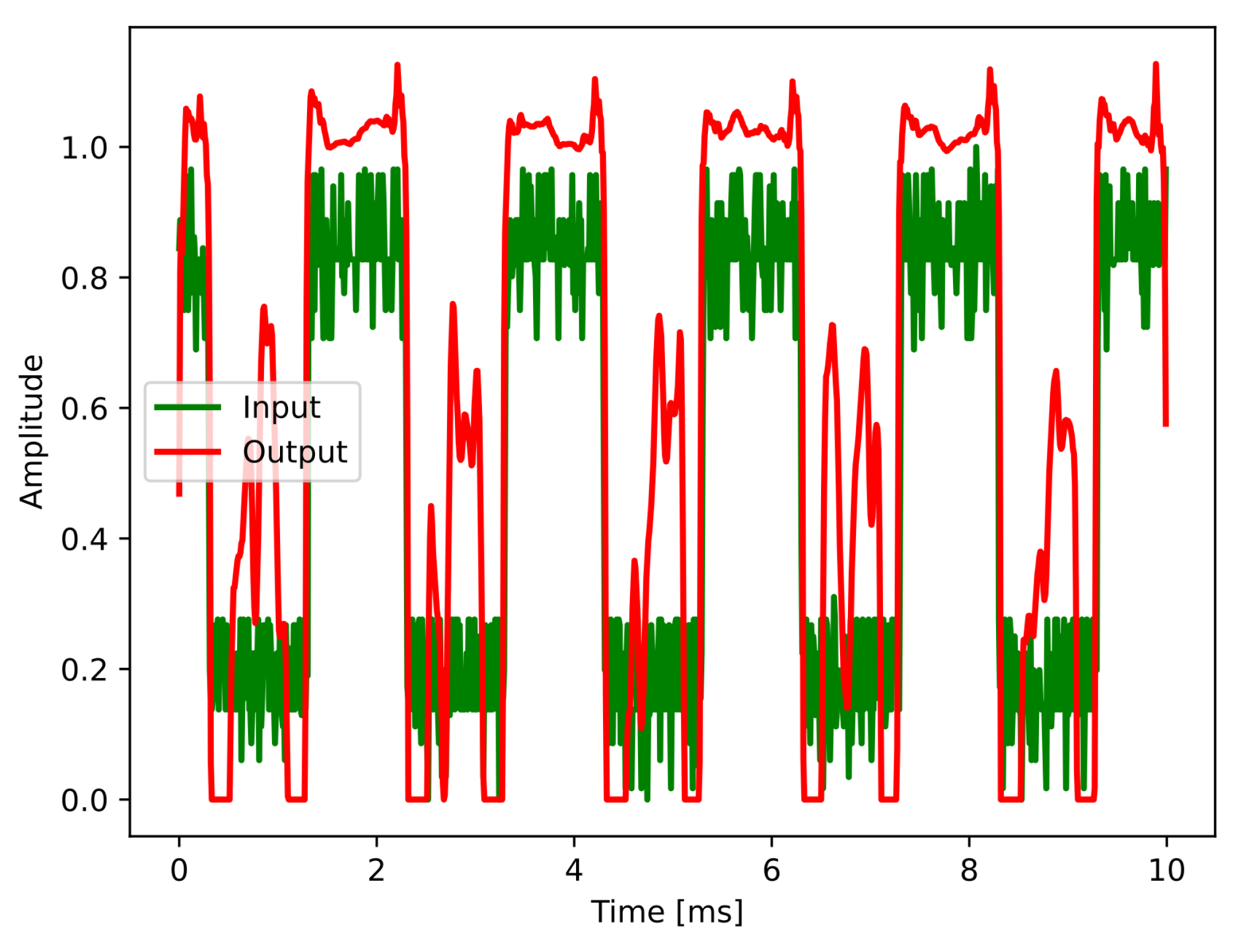
| Waveform | Time [secs] |
| Rectangular | 82.7 |
| Triangular | 82.2 |
| Sine | 81.5 |
Disclaimer/Publisher’s Note: The statements, opinions and data contained in all publications are solely those of the individual author(s) and contributor(s) and not of MDPI and/or the editor(s). MDPI and/or the editor(s) disclaim responsibility for any injury to people or property resulting from any ideas, methods, instructions or products referred to in the content. |
© 2024 by the authors. Licensee MDPI, Basel, Switzerland. This article is an open access article distributed under the terms and conditions of the Creative Commons Attribution (CC BY) license (http://creativecommons.org/licenses/by/4.0/).


