1. Introduction
Over recent years, there has been a growing interest in spiking neural networks (SNN) and spiking models, which have found applicability in various domains, such as pattern recognition and clustering, among others. Spiking neural networks, regarded as the third generation of artificial neural networks (ANN), differ from classic ANN by processing data as sequences of spikes known as spike trains. This implies that SNN, in terms of computation, only require a single bit line toggling between logical levels ’0’ and ’1’ in contrast to classic ANN that operate with real or integer-valued inputs. SNN excel in processing both temporal and spatial patterns, rendering them computationally more potent than ANN [
1].
Spiking neural networks (SNNs) transmit spike signals between neurons, operating as an event-driven or clock-driven computing systems where power consumption is primarily concentrated in the current active parts of the networks. This design allows for effective energy savings in inactive regions, enabling SNNs to perform distributed and asynchronous computing with minimized network time delays and enhanced real-time capabilities [
2,
3]. While Convolutional Neural Networks (CNNs) have proven highly successful for natural image classification [
4], their training and operational demands require substantial computing resources. Notably, SNNs demonstrate superior high-speed operational performance, in contrast to CNNs, which exhibit strengths in classification tasks.
While SNNs exhibit impressive computational capabilities, they still lack effective learning mechanisms aligned with biological processes [
5]. The predominant learning principle in SNNs, Spike-timing-dependent plasticity (STDP), proves inadequate for training multilayer neural networks. Consequently, there is a growing interest in the training approach for SNNs. This method involves initially training a conventional artificial neural network using the backpropagation algorithm. Subsequently, the network parameters, such as weights and biases, undergo conversion through suitable methods for utilization in SNNs. Various approaches have been explored to adapt existing neural networks to SNNs. Cao et al. customized a standard CNN to meet SNN requirements, albeit with some resulting performance losses [
6]. Diehl et al. [
7] improved network performance by converting a CNN to an SNN through weight normalization, reducing conversion errors. Hunsberger et al. [
8] enhanced conversion performance by incorporating Leaky Integrate-and-Fire (LIF) neurons into the SNN. Theoretically, SNNs can match or surpass the performance of CNNs [
9], yet achieving equivalent practical performance remains challenging.
There are examples of intelligent systems, converting data directly from sensors [
10,
11], controlling manipulators [
12] and robots [
13], doing recognition or detection tasks [
14,
15], tactile sensing [
16] or processing neuromedical data [
17]. Li et al. [
18] incorporated the mechanism of LIF neurons into the MLP models and propose a full-precision LIF operation to communicate between patches, including horizontal LIF and vertical LIF in different directions. The SNN-MLP model achieves 81.9%, 83.3% and 83.5% top-1 accuracy on ImageNet dataset with only 4.4G, 8.5G and 15.2G FLOPs. Zhang et al. [
19] proposed a multiscale dynamic coding improved spiking actor network (MDC-SAN) for reinforcement learning to achieve effective decision-making. The population coding at the network scale is integrated with the dynamic neurons coding at the neuron scale towards a powerful spatial-temporal state representation. Cuadrado et al. [
20] proposed a U-Net-like SNN encouraging both minimal norm for the error vector and minimal angle between ground-truth and predicted flow to make dense optical flow estimations. In addi-tion, the use of 3d convolutions contributed to capture the dynamic nature of the data by increasing the temporal receptive fields. Zou et al. [
21] dedicated end-to-end sparse deep learning approach for event-based pose tracking and achieved a computation reduction of 20% in FLOPS. It is based entirely upon the framework of Spiking Neural Networks (SNNs), which consists of Spike-Element-Wise (SEW) ResNet and a spiking spatiotemporal transformer.
Facial expression recognition is a pivotal field in computer comprehension of human emotions and a crucial element of human-computer interaction. It involves selecting facial expressions from static photos or video sequences to determine the emotional and psychological changes in individuals. In the 1970s, American psychologists Ekman and Friesen defined six fundamental human expressions through extensive experiments: happiness, anger, surprise, fear, disgust, and sadness.
However, recognizing such expressions under naturalistic conditions poses significant challenges due to variations in head pose, illumination, occlusions, and the nuanced nature of unposed expressions. The Facial Expression Recognition Challenge, as a prominent track in three machine learning contests, is notably demanding. For instance, a manual test conducted on the official Fer2013 dataset revealed that human recognition accuracy for the original dataset is approximately 65%. It is evident that label recognition is challenging even for humans. The official extraction of a small, clean subset from the original dataset resulted in a human recognition accuracy of around 68%.
The analysis of human face characteristics and the recognition of its emotional state are considered to be very challenging and difficult tasks. The main difficulty comes from the non-uniform nature of the human face and various limitations related to lighting, shadows, facial pose and orientation conditions [
22]. In the Large Scale Visual Recognition Challenge (ILSVRC) 2012, the AlexNet model, utilizing CNN, notably enhanced Facial Expression Recognition (FER) accuracy. Subsequently, more intricate CNN variants emerged like VGGNet [
23], GoogleNet [
24], and ResNet [
25]. However, these deep learning network models were complex and had a large number of parameters, making them unsuitable for embedded computers and mobile devices. It’s worth noting that current research on Spiking Neural Networks is still in the model exploration stage, with relatively fewer studies focusing on practical applications. Notably, there is a lack of research introducing SNNs into the field of facial expression recognition.
The structure of the paper is organized as follows. In Sect. 2, background topics on spiking neurons, the STDP fine-tune method, construction of convolutional SNN and its loss function are examined. Sect. 3, presents the experimental study conducted, examines the results collected and discusses the main findings. After that, Sect. 4, describes the feature visualization results of the SNN. Finally, Sect. 5 concludes the paper and draws directions for future work.
This paper makes several significant contributions: It proposes a highly efficient convolutional SNN capable of facial expression recognition. The method fully explores the SNN’s clock-driven and synaptic sparsity properties. It significantly reduces the model parameter while approaching the accuracy of ANNs, thereby reducing computational consumption and enhancing training speed. Moreover, the paper proposes a novel fine-tuning approach for SNNs based on Spike-Timing-Dependent Plasticity (STDP). This method effectively integrates unsupervised learning inspired by biological neural computation to enhance supervised learning in SNNs, improving recognition accuracy and model generalization.
2. Method
2.1. Spiking Neurons
The Leaky-Integrate-and-Fire (LIF) model [
26], originally introduced by Lapicque in 1907, stands as the predominant spiking neuron model in contemporary neuroscience. Its widespread adoption is attributed to its simplicity as a linear model. This simplicity not only facilitates quantitative investigations into neuron properties through analytical expressions of membrane potential but also allows for the precise simulation of spiking neural networks using clock-driven simulation strategies.
Within this model, the transfer of ions in biological neural systems is metaphorically represented through electronic transfers. The cell body, meanwhile, is simulated as an experiment using capacitance, enabling the storage of voltage. This dual capacity for quantitative analysis and accurate clock-driven simulation has solidified the LIF model’s enduring utility in the field of neural computation.
Similar to neurons in Recurrent Neural Networks (RNNs), spiking neurons also exhibit stateful behaviors, implying a form of memory. The state variable for spiking neurons is generally represented by their membrane potential, denoted as Vt. The membrane potential is influenced not only by the current input Xt but also by its membrane potential Vt-1 at the end of the previous time step.
The charging process of continuous-time spiking neurons is commonly characterized by a sub-threshold differential equation, which describes the charging dynamics when the membrane potential does not exceed the threshold voltage. For the Leaky-Integrate-and-Fire (LIF) model, the charging equation is typically employed as:
Where,
represents the membrane potential time constant, and
denotes the reset voltage. Due to the non-constant nature of
in the given differential equation, obtaining an explicit analytical solution proves challenging. Consequently, discrete difference equations are employed to approximate the continuous differential equation. From the perspective of the difference equation, the charging dynamics for the LIF neurons can be described as:
The expression of
can be derived as follows:
RNNs employ differentiable gating functions, such as the tanh function. On the other hand, SNNs utilize a non-differentiable spiking function. However, we can substitute it with a differentiable gating function that closely mimics a step function. This approximation maintains the behavior of a step function during forward propagation, returning 1 when the input is greater than or equal to 0, and 0 otherwise. During backward propagation, the gradient of the substituted function is used in place of the gradient of the spiking function. One commonly used substitute function is the adjustable sigmoid function , where governs the smoothness of the function. A higher makes the substitute function closer to the step function but increases the risk of gradient explosion near and gradient vanishing away from . This trade-off can impact the ease of training the network.
In SNNs, the forward propagation involves the use of a step function. We interpret these binary signals, representing either 0 or 1, as spikes. Releasing a spike depletes the charge accumulated by the neuron, leading to an instantaneous reduction in membrane potential, referred to as membrane potential reset. In SNNs, there are two approaches to implementing the reset of the membrane potential:
Hard Method: After releasing a spike, the membrane potential is immediately adjusted to the reset voltage;
Soft Method: After releasing a spike, the membrane potential undergoes a reduction equivalent to the threshold voltage;
Opting for the Hard Method enables the characterization of any discrete spiking neuron through three discrete equations: charging, discharging, and reset. This configuration resembles a step function
. The equations for charging and discharging are as follows:
The reset equation for the Hard Method is:
2.2. STDP Fine-Tune for SNN
Typically, the Hebbian learning rule updates synaptic weights based on the frequency of neuronal spike emissions. However, neuroscientific research has found that the encoding of spike frequency alone doesn’t fully capture the practical implications of synaptic plasticity. Instead, alterations in synaptic weights are closely tied to the precise timing of neuronal spike emissions, as observed by Markram et al. [
27]. In reality, the relative temporal difference between presynaptic and postsynaptic spike emissions plays a pivotal role in determining the direction and magnitude of synaptic changes. This learning rule, grounded in the temporal correlation of presynaptic and postsynaptic spike emissions, is termed Spike-timing-dependent plasticity (STDP), as elucidated by Caporale et al. [
28]. It can be considered as an expansion of the Hebbian learning rule.
Assuming a neural connection exists from presynaptic neuron i to postsynaptic neuron j, the STDP learning mechanism operates as follows:
(1) If a spike emitted by presynaptic neuron i reaches the synapse before postsynaptic neuron j generates a response spike, similar to a cause-and-effect relationship, the synaptic weight between the neurons strengthens.
(2) Conversely, if postsynaptic neuron j fires a spike before the presynaptic neuron transmits its own, rendering that information irrelevant, the synaptic weight between the neurons undergoes inhibition.
The spike sequence sent by presynaptic neurons i and postsynaptic neurons j are expressed as formula (7):
Where the is the delta function which sometimes called "spike symbol", and is the precise time of neuron spike.
In the study, it was observed that the changes in synaptic plasticity are not temporally symmetrical but instead arise from the temporal correlation of action potentials fired by presynaptic and postsynaptic neurons. The magnitude of synaptic weight adjustment
, is contingent upon the action potentials of both presynaptic and postsynaptic neurons, as well as the time difference between their spike emissions, denoted as
. The expression for the Spike-timing-dependent plasticity (STDP) function is as follows:
Where and represent the maximum values for synaptic strength enhancement and inhibition, both being positive values. The and correspond to the time constants for synaptic weight enhancement and weakening, respectively.
An elementary convolutional SNN is comprised of alternating convolutional and pooling layers followed by fully-connected layers. Some scholars have trained it with STDP-based unsupervised pre-training followed by supervised fine-tuning, but from the perspective of the SNN model initialization. We persist in our emphasis on supervised learning with convolutional SNN and proposed a method that utilizes STDP to fine-tune the network’s head for improved model generalization. Concretely, at intervals of every 10 training epochs, model weights are loaded. During the fine-tuning process, the convolutional and pooling layers are frozen, and STDP is applied to update the weights of the fully connected layer. This fine-tuning approach is consistently integrated throughout the entire training process.
2.3. Convolutional SNN
We propose a convolutional Spiking Neural Network for the classification of facial expression data. While most conventional Artificial Neural Networks (ANNs) commonly adopt a structure comprising convolutional and fully connected layers, our study replicates a similar architecture in the context of Spiking Neural Networks (SNNs). Leveraging the open-source spiking neural network framework, SpikingJelly [
29], we incorporate two convolutional-batch normalization-pooling layers and define a three-layer fully connected network to yield classification outcomes. In our experiments, it was observed that for static image data devoid of temporal information, neurons in the convolutional layer exhibited better performance when modeled using IFNode. Conversely, the fully connected layer, serving as a classifier, demonstrated superior performance when implemented with LIFNode.The framework diagram of the proposed SNN is shown in
Figure 1.
Utilizing a clock-driven methodology, the initial input of dimensions 1×48×48 undergoes processing through the first two convolutional layers, yielding an output spike of 128×12×12. Subsequently, the resulting vector is flattened for a 7-class classification. In experimental setups, images are directly input into the SNN. In this context, the spiking neurons of the first layer and the preceding layers receive input images that remain constant over time. For SNNs where input remains constant temporally, despite the overall statefulness of the SNN, the initial layers may lack temporal variation. These layers can be extracted and positioned outside the time loop to mitigate computational overhead. Simultaneously, the time loop is encapsulated within the network itself. The comprehensive structure and parameters of the proposed convolutional SNN are detailed in
Table 1.
2.4. Loss
After Gaussian distribution random initializing the SNN, we employ the Adam optimizer with a loss function that combines the spike firing rate of output layer neurons and Mean Squared Error (MSE) relative to the ground truth category. This loss function is designed to encourage the spike firing frequency of the i-th neuron in the output layer to approach 1 when input belongs to the i-th category, simultaneously driving the spike firing frequencies of other neurons towards 0. The loss function is expressed as follows:
Where x is the spike firing rate of output layer neurons and y is the ground truth category and N is the batch size.
3. Experiment Results
3.1. Dataset
The dataset employed in this study is the Fer2013 dataset [
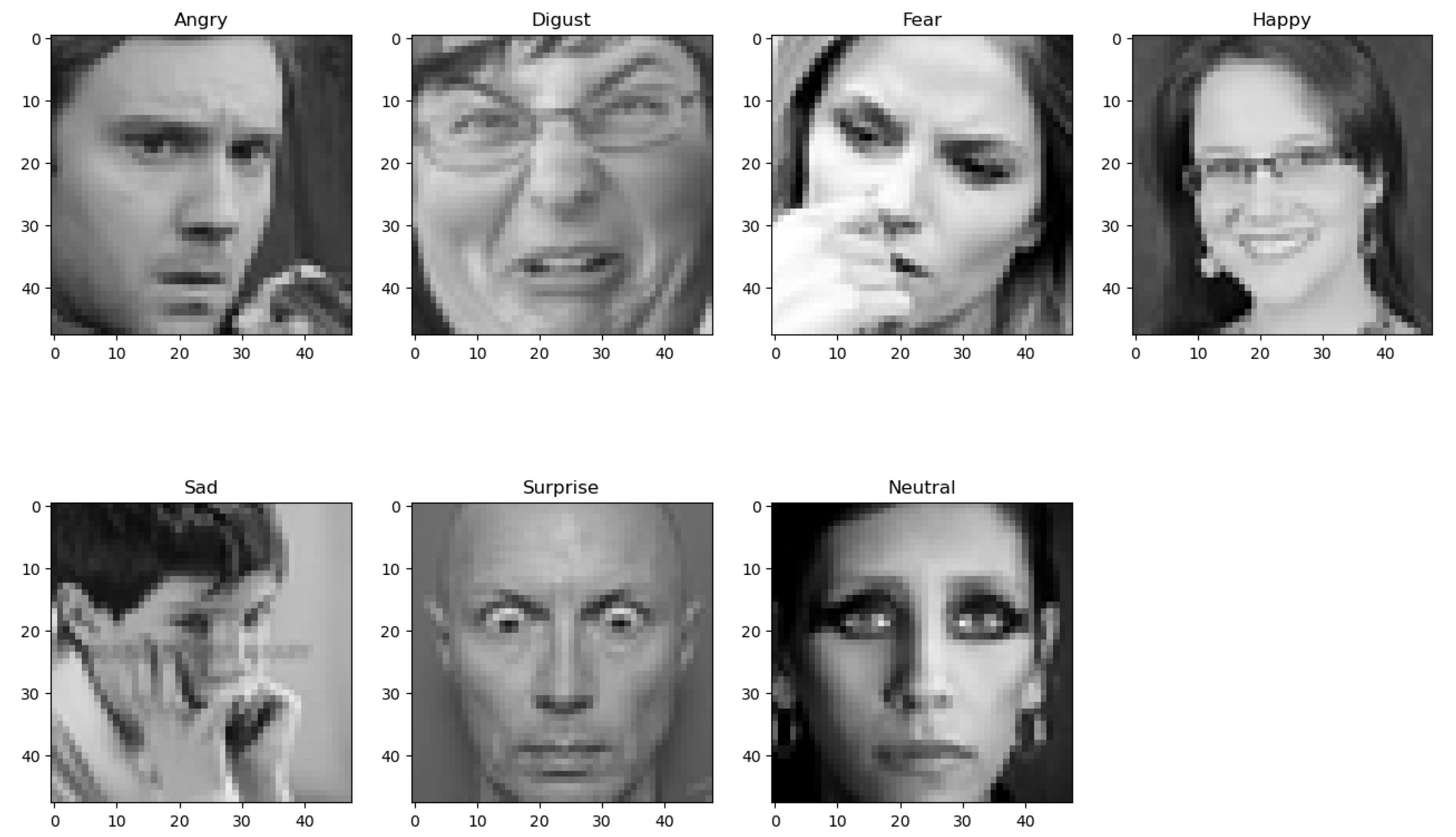
30], introduced at the 2013 International Conference on Machine Learning (ICML). It has since become a benchmark for evaluating the performance of facial expression recognition models and served as the dataset for the Kaggle Facial Expression Recognition Challenge in 2013. The Fer2013 dataset comprises 28,709 training images, 3,589 images in the public test set, and an additional 3,589 images in the private test set. Each image is a grayscale picture with dimensions of 48×48 pixels, as shown in
Figure 2, the Fer2013 dataset encompasses seven expression categories: angry, disgust, fear, happy, sad, surprise, and neutral. Notably, this dataset was primarily gathered through web scraping, introducing inherent inaccuracies and increasing the complexity of the training process.
Table 2 shows the data distribution of the Fer2013 dataset. The disgust expression has a minimal number of images of 547, while other categories have nearly 5,000 samples each.
Due to the presence of unexpected samples in the Fer2013 dataset, such as outliers that do not belong to any specific category, overfitting these samples could compromise the model’s generalization ability and, consequently, its overall performance. In this study, label smoothing is employed as a form of regularization during experiments. The Label smoothing introduces a certain level of noise to the one-hot distribution of labels, acting as a ’softening’ mechanism to prevent the model from being overly confident in its predictions and mitigating the risk of overfitting.
To ensure the experiment’s comprehensiveness, we incorporated the FER+ dataset [
31], which comes with updated annotations offering new labels for the standard Emotion FER dataset. Each image in FER+ has been annotated by 10 crowd-sourced taggers, providing higher-quality ground truth for still image emotions compared to the original FER labels. The inclusion of 10 taggers per image allows researchers to estimate emotion probability distributions per face, including additional categories such as contempt, unknown, and NF (Not a Face). This facilitates the development of algorithms capable of generating statistical distributions or multi-label outputs instead of the traditional single-label output.
3.2. Poisson Encoder
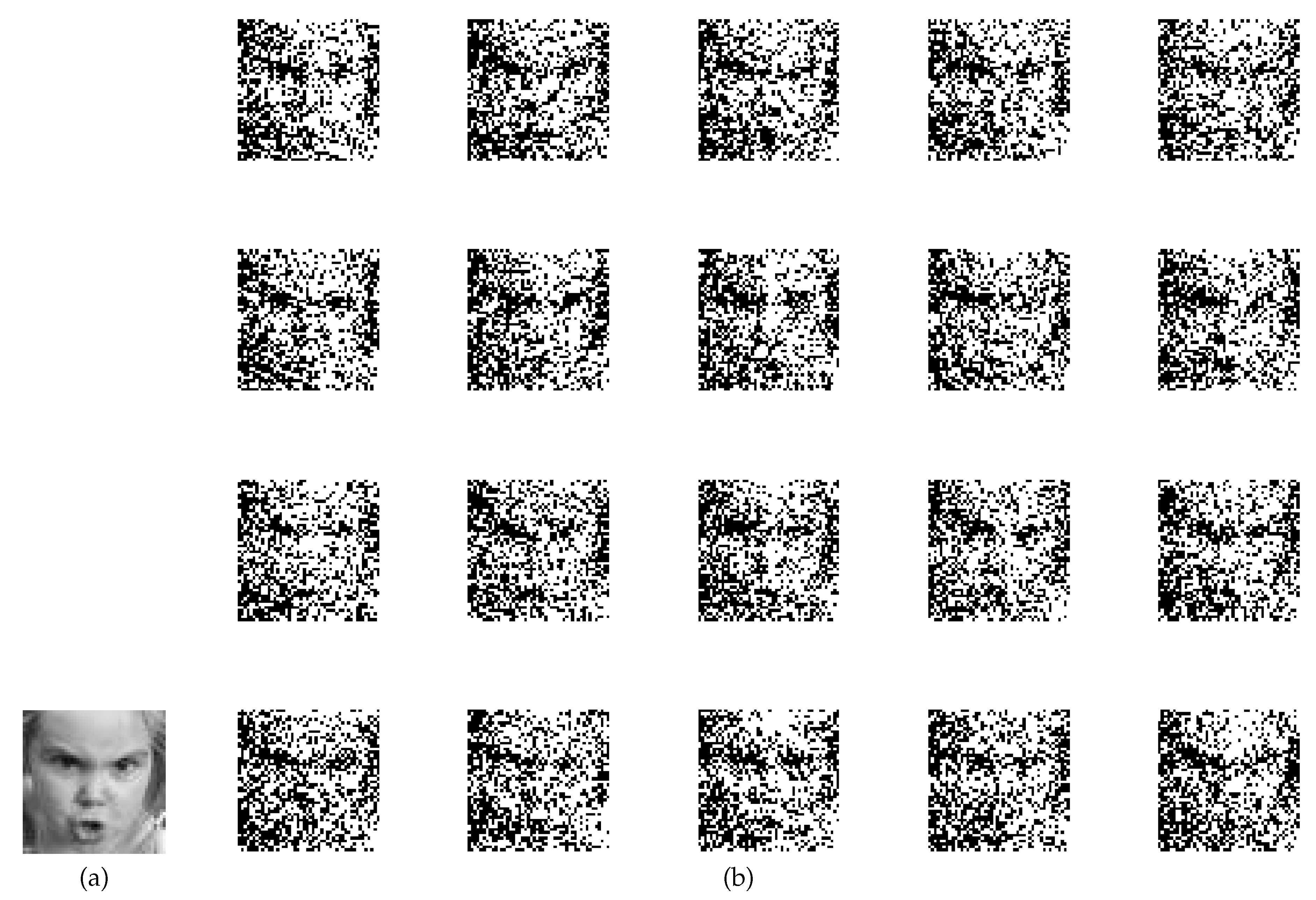
The Poisson encoder transforms input data into a spike sequence, adhering to a Poisson process where the spike count in a given period follows a Poisson distribution. This process, also referred to as a Poisson flow, satisfies conditions of independent increment, incremental stability, and commonality within the spike flow. Specifically, spikes appearing in disjoint intervals within the entire spike stream are independent of each other. Moreover, the spike count within any interval is solely dependent on the duration of the interval, not its starting point. To implement Poisson encoding, we set the firing probability of a time step p=x, with x normalized to the range [0, 1]. Using a "disgust" sample from the Fer2013 dataset, we simulated 20 time steps, resulting in 20 spike matrices. The original grayscale image of "disgust" and the corresponding 20 spike matrices are illustrated in
Figure 3.
The proximity of the spike matrix to the contour of the original grayscale image high-lights the effectiveness of the Poisson encoder. After simulating the Poisson encoder with the "disgust" grayscale image for 512 time steps, we overlayed the spike matrix obtained at each step. The resultant composite images, representing steps 1, 128, 256, 384, and 512, are depicted in
Figure 4.
Observing that with a sufficiently extended simulation, the original image can be nearly reconstructed using the composite images formed by overlaying spikes generated by the Poisson encoder.
3.3. Performance of Convolutional SNN and Comparison against the CNNs
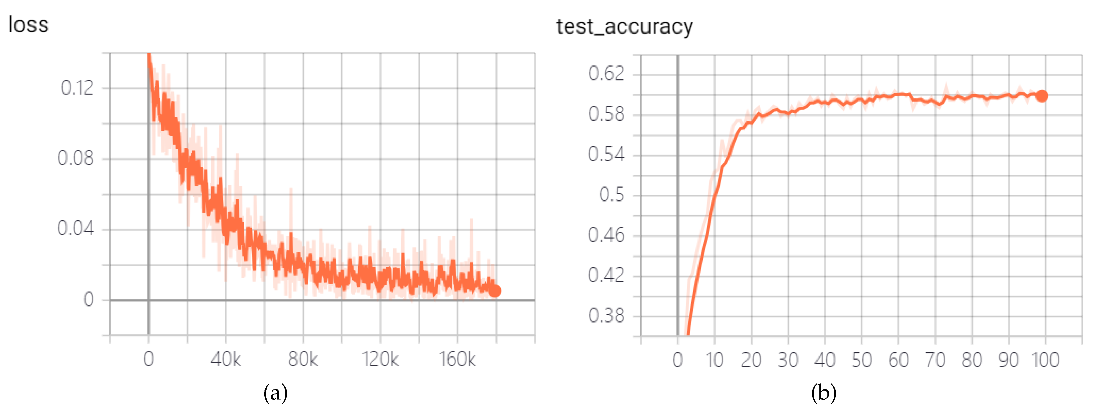
Firstly, the training for the Fer2013 dataset is performed using the proposed convolutional Spiking Neural Network without Poisson encoder and STDP fine-tune. The SNN hyperparameters are set as follows: batch size at 16, simulation time steps (T) at 4, and membrane potential time constant (
) of 2.0. The network with the highest accuracy on the test set during the training process is saved in the TensorBoard logs. The experimental outcomes are presented in
Figure 5.
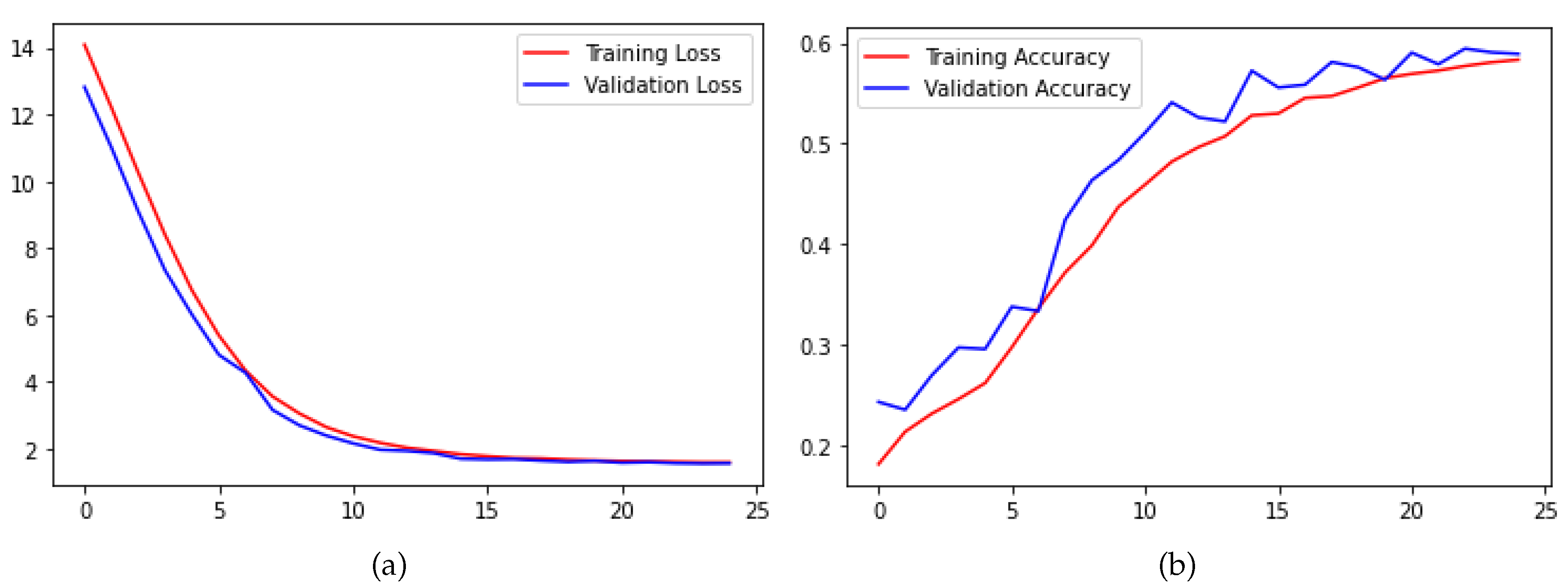
After 100 epochs of training, the highest accuracy on the test set reaches 60.15%, surpassing the 59.23% accuracy achieved by a similarly layered CNN composed of three convolutional layers followed by fully connected layers, which are shown in
Figure 6. Additionally, it only marginally lags behind the 66.21% accuracy achieved by MobileNet v1 [
32].
The experiment was conducted using an RTX 2060 Super GPU (8GB). Table II illustrates a comparative analysis between the convolutional SNN and a CNN with an equivalent number of layers, considering model parameter count, training speed, and computational efficiency.
Table 3 highlights that the convolutional Spiking Neural Network (SNN), compared to a CNN with an equivalent number of layers, demonstrates nearly a 60% reduction in total parameters. Moreover, its overall multiply-accumulate (MAC) operations decreased by one-third, accompanied by a model size reduction from 215.3 MB to 86.12 MB. When tested under identical hardware conditions, the CNN achieves a training speed of 152.38 fps, whereas the convolutional SNN achieves an impressive 398.73 fps, marking an approximate 2.6-fold enhancement. Notably, in GPU memory occupancy, the convolutional SNN model requires only about 81%, leading to an estimated energy efficiency of around 2.84 fps/w, showcasing a remarkable 3.46-fold improvement over the CNN model.
We examined four CNNs designed with architectures inspired by current state-of-the-art models in relevant domains. Our focus was not on finding architectures optimized for Fer2013 but rather on confirming the general effectiveness of modern deep architectures. As listed in
Table 4, even with a shallow design, SNNs showcase the ability to approach the model accuracy of their counterparts. The proposed convolutional SNN demonstrates competitive model accuracy compared to shallow CNNs.
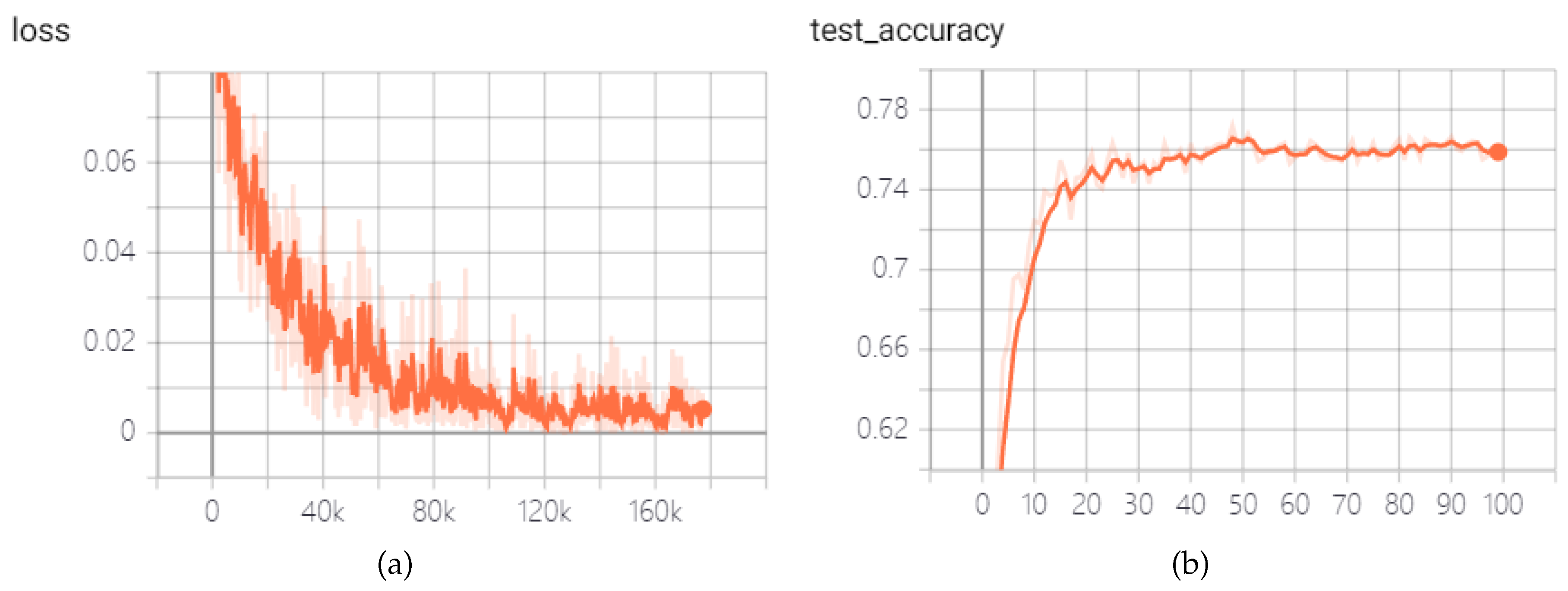
To achieve a more generalized SNN model, we excluded images from the FER+ dataset belonging to the ’unknown’ and ’NF’ categories. We adopted the majority emotion as the sole emotion label and evaluated prediction accuracy based on the majority emotion. The proposed convolutional SNN achieved a 77.17% accuracy on the FER+ dataset after 100 training epochs with consistent hyperparameters, as depicted in
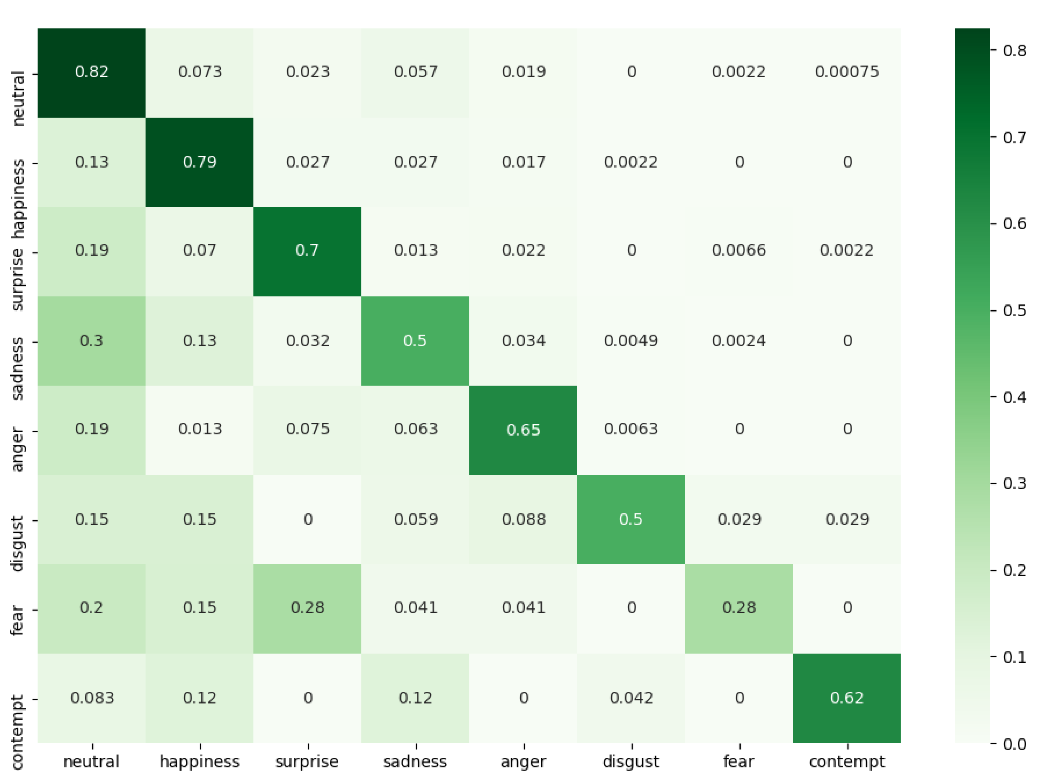
Figure 7. The corresponding confusion matrix in
Figure 8 illustrates the SNN network’s performance, show-casing proficiency in most emotions except for fear. This discrepancy is attributed to the high similarity between fear and surprise expressions, compounded by a lower quantity of fear samples in the FER+ dataset.
3.4. Sparse Weights of SNN and Comparison against the CNN Pruning
In deep neural networks, a substantial portion of activation values is either unnecessary (set to 0) or redundant due to correlations. Therefore, the most efficient architecture for deep networks should exhibit sparse connections among activation values. Model pruning methods, known for significantly reducing both model parameters and computational workload, have become a predominant approach for compressing models. On one hand, inspired by the findings in [
36], we conducted sparse training on the
parameters of the Batch Normalization (BN) layer in the VGG network. After obtaining the corresponding mask, we pruned the Conv2d, Batch Normalize, and Linear layers, resulting in a reduction of the model’s parameter count from 71 million to 9.6 million, achieving a model size reduction ratio of approximately 8 times.
On the other hand, the native SNN model proposed by Chen et al. [
37]. indicates that its model parameter count can be reduced by approximately 30 times compared to CNNs. Therefore, leveraging the robust sparsity in the transmission of pulse signals between neurons, SNNs excel in reducing model parameter count compared to pruning methods.
Pruning methods typically involve three steps: large-scale model training and pruning, followed by fine-tuning of the pruned small-scale model. When the pruning rate is excessively high, small-scale models obtained through existing pruning methods may suffer from severe information loss and insufficient semantic expressive capability, leading to significant accuracy loss. Under such circumstances, SNN models will demonstrate unparalleled advantages.
3.5. Ablation Studies
1) With or without Poisson encoding: The Poisson encoder is a method employed in SNNs for converting continuous input signals into spike trains. The Poisson process introduces inherent variability or noise in the spike generation, which can contribute to the network’s robustness against input variations and noise. This stochasticity can help SNNs handle uncertain or dynamic input patterns effectively. Meanwhile, the Poisson encoder facilitates dynamic adaptation to changing input conditions. As the encoding is probabilistic, it can naturally adjust to varying input statistics, making SNNs suitable for tasks that involve non-stationary input patterns.
2) With or without STDP fine-tune: We utilized STDP fine-tune for adjusting synaptic weights based on the timing of spikes between connected neurons in the fully connection layers. STDP is sensitive to precise spike timings, allowing for fine-tune of synaptic weights based on the temporal proximity of pre-synaptic and post-synaptic spikes. This temporal sensitivity contributes to the network’s ability to capture temporal information in data. Moreover, STDP allows SNNs to adapt to changing input patterns and dynamic environments. As the network continuously learns and updates synaptic weights based on incoming spike timings, it can adapt to new information and changing input statistics. It tends to induce sparse connectivity patterns by strengthening selective connections based on spike timing correlations. This sparsity contributes to more efficient representation and processing of information within the network.
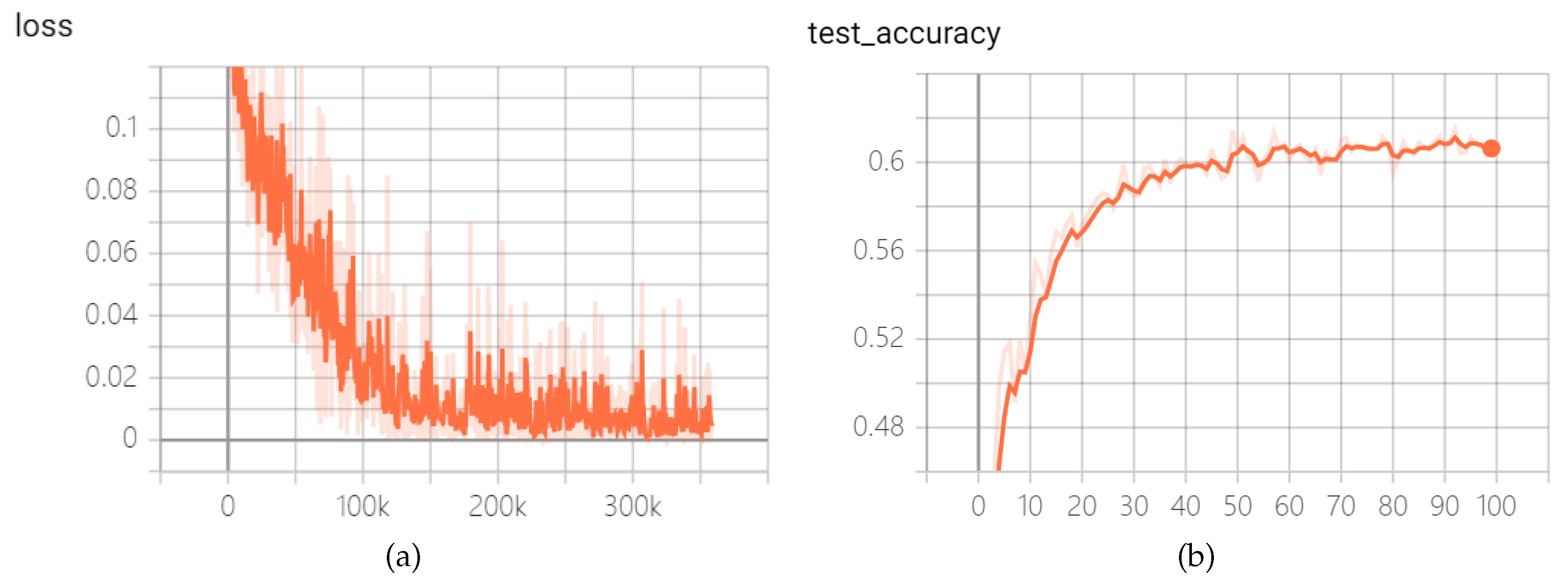
In this study, we conducted three supplementary experiments to enhance the training of a convolutional SNN that directly processes images. Specifically, we increased simulation time steps and introduced Poisson encoder and STDP fine-tune for the fully connected layers. Under identical SNN hyperparameters,
Figure 9 illustrates the training and testing accuracy curves of the convolutional SNN of simulation time steps T=8 and with Poisson encoder and STDP fine-tune on the Fer2013 dataset. In comparison to the convolutional SNN discussed in Section C, the testing accuracy demonstrated a further improvement of 1.72%, reaching a final accuracy of 61.87%. In the proposed clock-driven approach, the STDP algorithm precisely adjusts synaptic weights exclusively within the fully connected layer. This algorithm operates swiftly, incurring no notable increase in computational time. A comparison between
Figure 9 and
Figure 5 indicates that STDP fine-tuning effectively lowered the loss and expedited the descent process. Moreover, the aforementioned refinements play a pivotal role in enhancing the training stability and adaptability of the convolutional SNN in dynamic environments.
The performance of SNN is sensitive to its hyperparameters. The hyperparameters need to be debugged according to the LIF model‘s biological characteristics and the data set. The specific values of the hyperparameters for the convolutional SNN and STDP fine-tune are listed in Table IV.
Under identical SNN hyperparameters,
Table 6 presents the classification accuracy comparison of several convolutional SNN variants on the Fer2013 dataset and the FER+ dataset. The findings validate performance improvements in the convolutional SNNs attributed to both the Poisson encoder and STDP fine-tune, resulting in respective accuracy boosts of 0.76% and 0.96% on the Fer2013 dataset and 1.62% and 1.18% on the FER+ dataset.
4. Feature Visualization Results
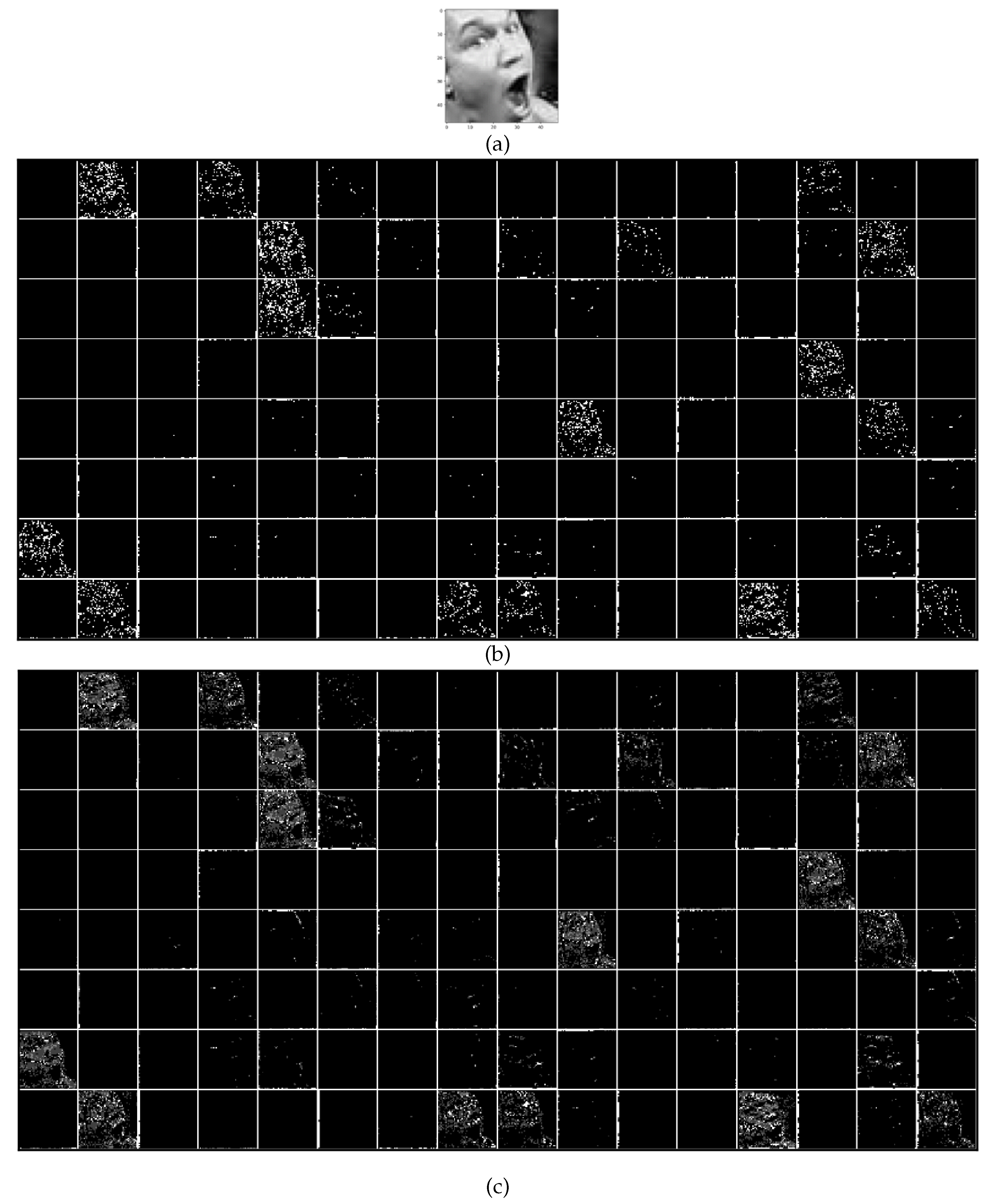
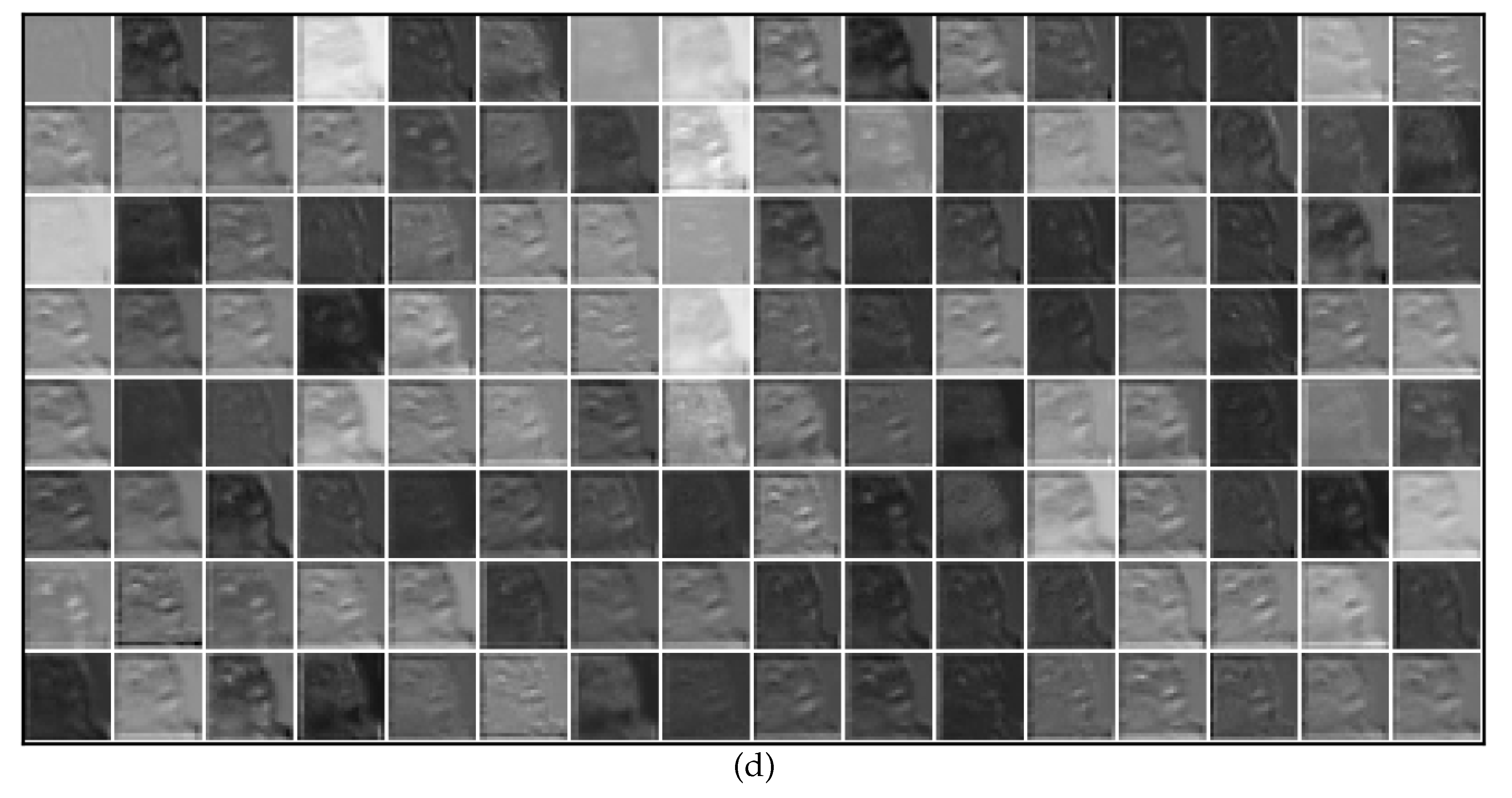
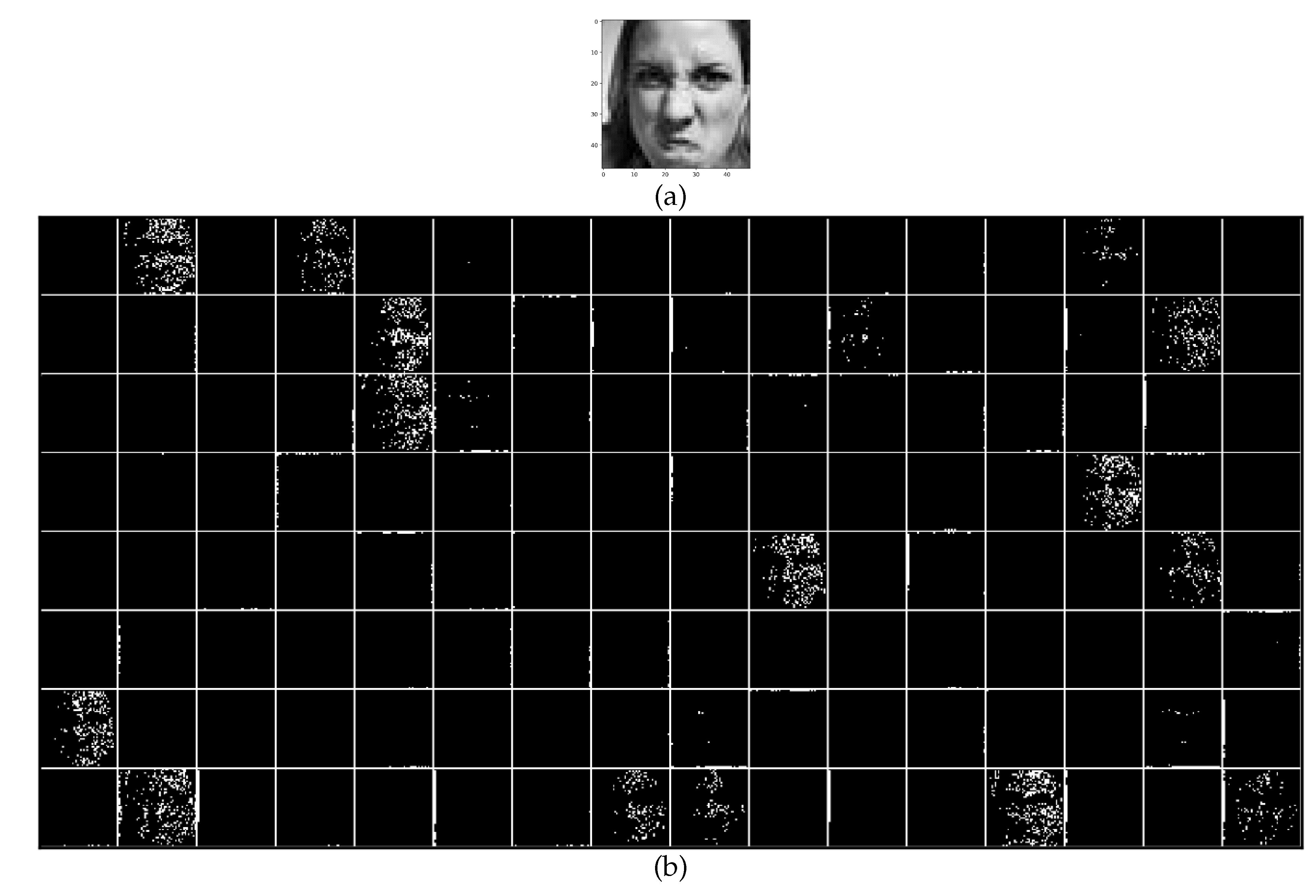
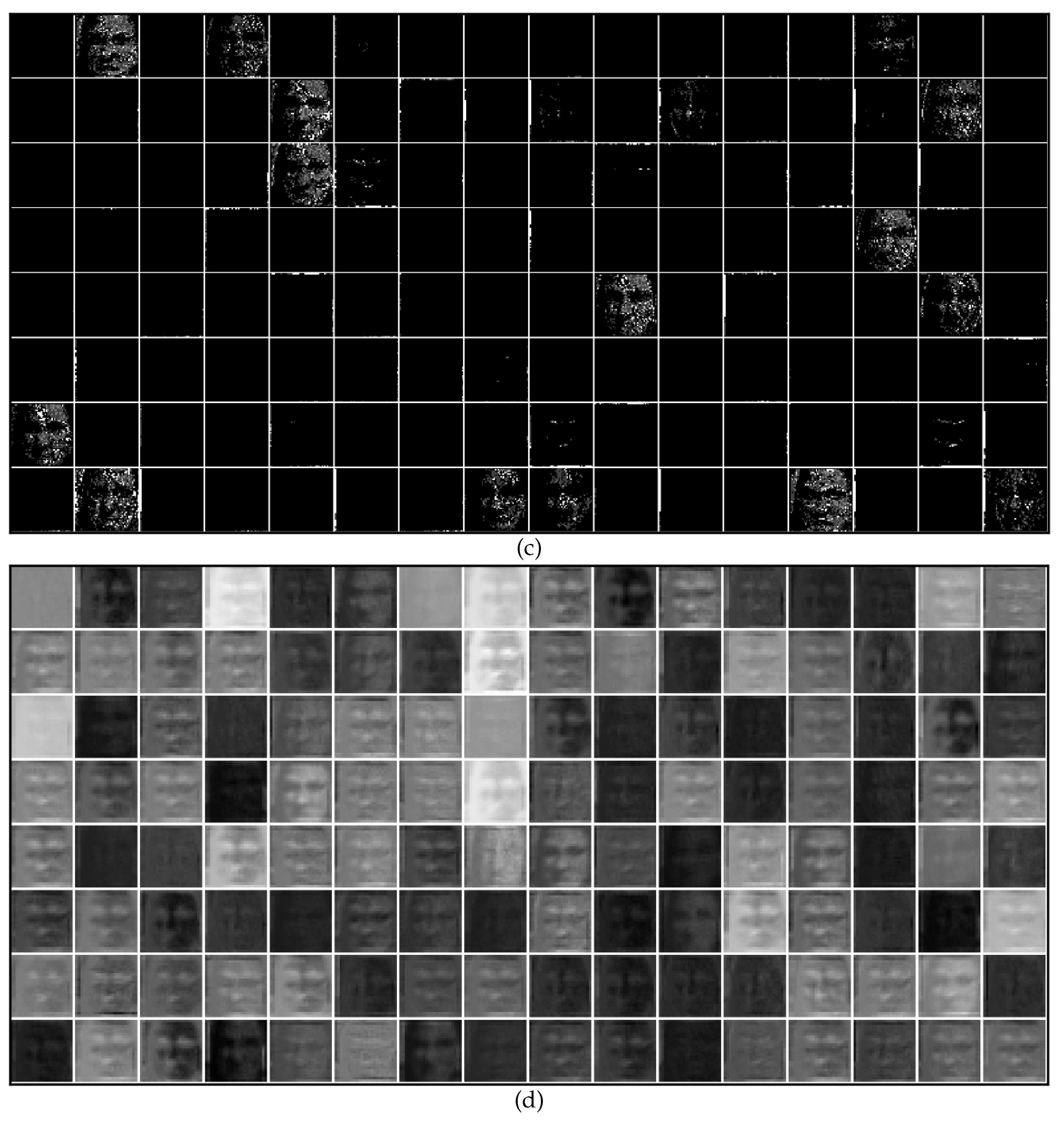
Regarding feature map visualization, when feeding data directly into the convolutional SNN, the first spiking layer and the layers preceding it can be viewed as a trainable encoder, denoted as Encoder I. Encoder II refers to the network extending from the second convolutional layer to just before the fully connected layer.
In order to review images individually, we have redefined a data loader with a batch size of 1. We loaded the pre-trained model, extracted the encoder, and ran it on the CPU. The cumulative spike outputs
of Encoder I and Encoder II are examined, with pixel values of the output feature maps normalized for clarity through a linear transformation to the range [0, 1].
Figure 10 and
Figure 11 illustrates two input images along with the cumulative spikes from Encoder I and Encoder II at the start time step (t=0) and the final time step (t=3).
Figure 10.
Feature visualization of convolutional SNN, example 1: (a) Input image. (b) Cumulative spikes of Encoder I at t=0. (c) Cumulative spikes of Encoder I at t=3. (d) Cumulative spikes of Encoder II at t=3.
Figure 10.
Feature visualization of convolutional SNN, example 1: (a) Input image. (b) Cumulative spikes of Encoder I at t=0. (c) Cumulative spikes of Encoder I at t=3. (d) Cumulative spikes of Encoder II at t=3.
Figure 11.
Feature visualization of convolutional SNN, example 2: (a) Input image. (b) Cumulative spikes of Encoder I at t=0. (c) Cumulative spikes of Encoder I at t=3. (d) Cumulative spikes of Encoder II at t=3.
Figure 11.
Feature visualization of convolutional SNN, example 2: (a) Input image. (b) Cumulative spikes of Encoder I at t=0. (c) Cumulative spikes of Encoder I at t=3. (d) Cumulative spikes of Encoder II at t=3.
The feature visualization results indicated a remarkable resemblance between the cumulative output spike pattern generated by the encoder and the contour of the original image. It implied that the self-learning spike encoder exhibits robust coding capabilities.
5. Discussion
On one hand, pulse sequences inherently incorporate temporal information, allowing for a more precise simulation of the dynamic processes of neurons over time. On the other hand, deep neural networks often exhibit redundant activation values due to correlations, suggesting that the most efficient architectures should feature sparse connections between activations. The proposed native SNN model in this study shows a parameter reduction of over two-fold compared to CNNs. Hence, leveraging the robust sparsity in pulse signal transmission between neurons, SNNs outperform pruning methods significantly in reducing model parameters. Additionally, this leads to a substantial decrease in computational power consumption.
Furthermore, Poisson encoding and header STDP fine-tuning can further elevate model performance. Spiking neural networks emulate the information transmission mechanisms of the brain by learning the interaction patterns between presynaptic and postsynaptic neurons, thus offering strong biological interpretability. Visualizing convolutional SNN feature maps reveals that longer simulation durations correlate with more precise feature extraction.
Future research directions primarily focus on two aspects: first, expanding the applicability of the proposed model to verify its reliability and generalization in broader scenarios; second, integrating spiking neural networks with neuromorphic chips to achieve higher computational efficiency and lower energy consumption.
6. Conclusions
This article constructed a lightweight shallow convolutional Spiking Neural Network (SNN) utilizing the SpikingJelly open-source platform for facial expression recognition. By integrating the Poisson encoder and Spike-Timing-Dependent Plasticity (STDP) fine-tune, the respective accuracy on the Fer2013 dataset and FER+ dataset reaches 61.87% and 79.97%, demonstrating competitiveness with CNNs of an equivalent number of layers. The encoding proficiency of the proposed convolutional SNN is powerfully demonstrated through visualizations of the encoder. Exploiting the inherent sparsity of spike sequences, the proposed convolutional SNN exhibits advantages, including low energy consumption and high computational efficiency, approximately three times more efficient than artificial neural networks. We broke away from the constraints of conventional facial expression recognition models by incorporating convolutional SNN into the field, marking a pioneering and valuable application of SNN algorithms.
Author Contributions
Conceptualization, Guiyang Pu and Rui Wang; methodology, Guiyang Pu and Jiankun Chen; software, Jiankun Chen; validation, Guiyang Pu and Jiankun Chen; formal analysis, Guiyang Pu and Rui Wang; investigation, Guiyang Pu; resources, Guiyang Pu and Rui Wang; data curation, Jiankun Chen; writing—original draft preparation, Jiankun Chen; writing—review and editing, Guiyang Pu; visualization, Jiankun Chen; supervision, Guiyang Pu and Zhongcai Tang; project administration, Guiyang Pu and Zhongcai Tang; funding acquisition, Guiyang Pu. All authors have read and agreed to the published version of the manuscript.
Funding
This research was funded by the Zhejiang Province’s 2023 ’Pioneer’ Key Research and Development Program of Zhejiang provincial department of science and technology, China, grant number 2023C01041.
Institutional Review Board Statement
Not applicable.
Informed Consent Statement
Not applicable.
Data Availability Statement
The public datasets are contained within the article.
Acknowledgments
The authors thank Lianzhen Zhong for debugging the code in the feature map visualization section of this experiment. The authors are also grateful to the IEEE Senior Member of Xiaolan Qiu, Aerospace Information Research Institute, Chinese Academy of Sciences, for the recommend of SpikingJelly. Finally, a special thank you to the anonymous reviewers for their invaluable comments and suggestions.
Conflicts of Interest
The authors declare no conflicts of interest.
Abbreviations
The following abbreviations are used in this manuscript:
| SNN |
Spiking Neural Network |
| STDP |
Spike Timing Dependent Plasticity |
| LIF |
Leaky Integrate-and-Fire |
| FER |
Facial Expression Recognition |
| MSE |
Mean Squared Error |
References
- Maass, Wolfgang. Networks of spiking neurons: the third generation of neural network models. Neural networks 1997, 10, 1659–1671. [Google Scholar] [CrossRef]
- Neftci E O, Pedroni B U, Joshi S, et al. Stochastic synapses enable efficient brain-inspired learning machines. Frontiers in neuroscience 2016, 10, 185771. [Google Scholar]
- Folowosele F, Vogelstein R J, Etienne-Cummings R. Real-time silicon implementation of V1 in hierarchical visual information processing. 2008 IEEE Biomedical Circuits and Systems Conference. IEEE 2008, 181–184.
- LeCun Y, Bottou L, Bengio Y, et al. Gradient-based learning applied to document recognition. Proceedings of the IEEE 1998, 86, 2278–2324. [CrossRef]
- Brader J M, Senn W, Fusi S. Learning real-world stimuli in a neural network with spike-driven synaptic dynamics. Neural computation 2007, 19, 2881–2912. [CrossRef] [PubMed]
- Cao Y, Chen Y, Khosla D. Spiking deep convolutional neural networks for energy-efficient object recognition. International Journal of Computer Vision 2015, 113, 54–56. [Google Scholar] [CrossRef]
- Diehl P U, Neil D, Binas J, et al. Fast-classifying, high-accuracy spiking deep networks through weight and threshold balancing. 2015 International joint conference on neural networks (IJCNN). IEEE 2015, 1–8.
- Hunsberger E, Eliasmith C. Spiking deep networks with LIF neurons. arxiv, 2015; arXiv:1510.08829.
- Maass W, Markram H. On the computational power of circuits of spiking neurons. Journal of computer and system sciences 2004, 69(4), 593–616. [Google Scholar] [CrossRef]
- Lovelace J J, Rickard J T, Cios K J. A spiking neural network alternative for the analog to digital converter. The 2010 International Joint Conference on Neural Networks (IJCNN). IEEE; 2010; pp. 1–8.
- Ambard M, Guo B, Martinez D, et al. A spiking neural network for gas discrimination using a tin oxide sensor array. 4th IEEE International Symposium on Electronic Design, Test and Applications (delta 2008). IEEE; 2008; pp. 394–397.
- Bouganis A, Shanahan M. Training a spiking neural network to control a 4-dof robotic arm based on spike timing-dependent plasticity. The 2010 International Joint Conference on Neural Networks (IJCNN). IEEE; 2010; pp. 1–8.
- Alnajjar F, Murase K. Sensor-fusion in spiking neural network that generates autonomous behavior in real mobile robot. 2008 IEEE International Joint Conference on Neural Networks; 2008; pp. 2200–2206.
- Perez-Carrasco JA, Acha B, Serrano C, Camunas-Mesa L, Serrano-Gotarredona T, Linares-Barranco B. Fast vision through frameless event-based sensing and convolutional processing: Application to texture recognition. IEEE transactions on neural networks 21, 609–620. [CrossRef] [PubMed]
- Botzheim J, Obo T, Kubota N. Human gesture recognition for robot partners by spiking neural network and classification learning. The 6th International Conference on Soft Computing and Intelligent Systems, and The 13th International Symposium on Advanced Intelligence Systems. IEEE; 2012; 19, pp. 1954–1958.
- Ratnasingam S, McGinnity T M. A spiking neural network for tactile form based object recognition. The 2011 International Joint Conference on Neural Networks. IEEE; 2011; pp. 880–885. [Google Scholar]
- Fang H, Wang Y, He J. Spiking neural networks for cortical neuronal spike train decoding. Neural Computation 2010, 22(4), 1060–1085. [Google Scholar] [CrossRef] [PubMed]
- Li W, Chen H, Guo J, et al. Brain-inspired multilayer perceptron with spiking neurons. In Proceedings of the IEEE/CVF Conference on Computer Vision and Pattern Recognition. 2022; pp. 783–793.
- Zhang D, Zhang T, Jia S, et al. Multi-sacle dynamic coding improved spiking actor network for reinforcement learning. Proceedings of the AAAI Conference on Artificial Intelligence. 2022; 36, 59–67.
- Cuadrado J, Rançon U, Cottereau B R, et al. Optical flow estimation from event-based cameras and spiking neural networks. Frontiers in Neuroscience. 2023, 17, 1160034. [Google Scholar] [CrossRef] [PubMed]
- Zou S, Mu Y, Zuo X, et al. Event-based human pose tracking by spiking spatiotemporal transformer. arxiv, arXiv:2303.09681.
- Krizhevsky A, Sutskever I, Hinton G E. ImageNet classification with deep convolutional neural networks. Communications of the ACM 2017, 60(6), 84–90. [Google Scholar] [CrossRef]
- Simonyan K, Zisserman A. Very deep convolutional networks for large-scale image recognition. arxiv, 2014; arXiv:1409.1556.
- Szegedy C, Liu W, Jia Y, et al. Going deeper with convolutions. Proceedings of the IEEE conference on computer vision and pattern recognition, 2015, 1–9.
- He K, Zhang X, Ren S, et al. Deep residual learning for image recognition. Proceedings of the IEEE conference on computer vision and pattern recognition, 2016, 770–778.
- Wang Z, Guo L, Adjouadi M. A generalized leaky integrate-and-fire neuron model with fast implementation method. International journal of neural systems 2014, 24, 1440004. [CrossRef] [PubMed]
- Markram H, Lübke J, Frotscher M, et al. Regulation of synaptic efficacy by coincidence of postsynaptic APs and EPSPs. Science 1997, 275, 213–215. [CrossRef] [PubMed]
- Markram H, Lübke J, Frotscher M, et al. Spike timing–dependent plasticity: a Hebbian learning rule. Annu. Rev. Neurosci., 2008, 31, 25–46. [Google Scholar] [CrossRef] [PubMed]
- Fang W, Chen Y, Ding J, et al. SpikingJelly: An open-source machine learning infrastructure platform for spike-based intelligence. Science Advances 2023, 9, eadi1480. [CrossRef] [PubMed]
- Carrier P L, Courville A. Challenges in representation learning: Facial expression recognition challenge. Kaggle Competition, 2013.
- Barsoum E, Zhang C, Ferrer C C, et al. Training deep networks for facial expression recognition with crowd-sourced label distribution. Proceedings of the 18th ACM international conference on multimodal interaction, 2016; 279–283.
- Howard A G, Zhu M, Chen B, et al. Mobilenets: Efficient convolutional neural networks for mobile vision applications. arxiv, 2017; arXiv:1704.04861.
- Simonyan K, Zisserman A. Very deep convolutional networks for large-scale image recognition. arxiv, 2017; arXiv:1409.1556, 2014.
- He K, Zhang X, Ren S, et al. Deep residual learning for image recognition. Proceedings of the IEEE conference on computer vision and pattern recognition 2016, 770–778. [Google Scholar]
- Szegedy C, Liu W, Jia Y, et al. Going deeper with convolutions. Proceedings of the IEEE conference on computer vision and pattern recognition 2015, 1–9. [Google Scholar]
- Liu Z, Li J, Shen Z, et al. Learning efficient convolutional networks through network slimming. Proceedings of the IEEE international conference on computer vision 2017, 2736–2744. [Google Scholar]
- Chen J, Qiu X, Ding C, et al. SAR image classification based on spiking neural network through spike-time dependent plasticity and gradient descent. ISPRS Journal of Photogrammetry and Remote Sensing 2022, 188, 109–124. [Google Scholar] [CrossRef]
Figure 1.
The framework diagram of the proposed SNN for facial expression recognition.
Figure 1.
The framework diagram of the proposed SNN for facial expression recognition.
Figure 2.
Samples of seven expression categories in the Fer2013 dataset.
Figure 2.
Samples of seven expression categories in the Fer2013 dataset.
Figure 3.
The results of spike encoding in Poisson encoder: (a) The original grayscale image of “disgust”. (b) 20 resulting spike matrices.
Figure 3.
The results of spike encoding in Poisson encoder: (a) The original grayscale image of “disgust”. (b) 20 resulting spike matrices.
Figure 4.
The superimposed images of the grayscale image “disgust” composed of spikes obtained by the Poisson encoder.
Figure 4.
The superimposed images of the grayscale image “disgust” composed of spikes obtained by the Poisson encoder.
Figure 5.
Curves of loss and test accuracy of the convolutional SNN of simulation time steps T=4 but without Poisson encoder and STDP fine-tune in the Fer2013 dataset: (a) Loss. (b) Test accuracy.
Figure 5.
Curves of loss and test accuracy of the convolutional SNN of simulation time steps T=4 but without Poisson encoder and STDP fine-tune in the Fer2013 dataset: (a) Loss. (b) Test accuracy.
Figure 6.
Curves of loss, train accuracy and test accuracy of the CNN network, consisting of three layers of convolution followed by fully connected layers, in the Fer2013 dataset: (a) Loss. (b) Test accuracy.
Figure 6.
Curves of loss, train accuracy and test accuracy of the CNN network, consisting of three layers of convolution followed by fully connected layers, in the Fer2013 dataset: (a) Loss. (b) Test accuracy.
Figure 7.
Curves of loss, train accuracy and test accuracy of the CNN network, consisting of three layers of convolution followed by fully connected layers, in the Fer2013 dataset: (a) Loss. (b) Test accuracy.
Figure 7.
Curves of loss, train accuracy and test accuracy of the CNN network, consisting of three layers of convolution followed by fully connected layers, in the Fer2013 dataset: (a) Loss. (b) Test accuracy.
Figure 8.
Curves of loss and test accuracy of the convolutional SNN of simulation time steps T=4 but without Poisson encoder and STDP fine-tune in the FER+ dataset: (a) Loss. (b) Test accuracy.
Figure 8.
Curves of loss and test accuracy of the convolutional SNN of simulation time steps T=4 but without Poisson encoder and STDP fine-tune in the FER+ dataset: (a) Loss. (b) Test accuracy.
Figure 9.
Curves of loss and test accuary of the convolutional SNN of simulation time steps T=8 and with Poisson encoder and STDP fine-tune in the Fer2013 dataset: (a) Loss. (b) Test accuracy.
Figure 9.
Curves of loss and test accuary of the convolutional SNN of simulation time steps T=8 and with Poisson encoder and STDP fine-tune in the Fer2013 dataset: (a) Loss. (b) Test accuracy.
Table 1.
The structure and parameters of the proposed convolutional Spiking Neural Network (SNN).
Table 1.
The structure and parameters of the proposed convolutional Spiking Neural Network (SNN).
| Layer (type:depth-idx) |
Output Shape |
Param |
| Poisson encoder (alternative) |
– |
– |
| Sequential: 1-1 |
[1, 128, 48, 48] |
– |
| Conv2d: 2-1 |
[1, 128, 48, 48] |
1,152 |
| BatchNorm2d: 2-2 |
[1, 128, 48, 48] |
256 |
| Sequential: 1-2 |
[1, 128, 12, 12] |
– |
| IFNode: 2-3 |
[1, 128, 48, 48] |
– |
| MaxPool2d: 2-4 |
[1, 128, 24, 24] |
– |
| Conv2d: 2-5 |
[1, 128, 24, 24] |
147,456 |
| BatchNorm2d: 2-6 |
[1, 128, 24, 24] |
256 |
| IFNode: 2-7 |
[1, 128, 24, 24] |
– |
| MaxPool2d: 2-8 |
[1, 128, 12, 12] |
– |
| Sequential: 1-3 |
[1, 7] |
– |
| Flatten: 2-9 |
[1, 18432] |
– |
| Dropout: 2-10 |
[1, 18432] |
– |
| Linear: 2-11 |
[1, 1152] |
21,233,664 |
| LIFNode: 2-12 |
[1, 1152] |
– |
| Dropout: 2-13 |
[1, 1152] |
– |
| Linear: 2-14 |
[1, 128] |
147,456 |
| LIFNode: 2-15 |
[1, 128] |
– |
| Linear: 2-16 |
[1, 7] |
896 |
| LIFNode: 2-17 |
[1, 7] |
– |
| STDP fine-tune (alternative) |
– |
– |
Table 2.
The data distribution of the Fer2013 dataset.
Table 2.
The data distribution of the Fer2013 dataset.
| Expression |
Angry |
Fear |
Sad |
Neutral |
Happy |
Surprise |
Disgust |
| Number of samples |
4953 |
5121 |
6077 |
6198 |
8989 |
4002 |
547 |
Table 3.
Comparison of parameter-level energy efficiency between convolutional SNN and a CNN with an equivalent number of layers.
Table 3.
Comparison of parameter-level energy efficiency between convolutional SNN and a CNN with an equivalent number of layers.
| Title 1 |
Convolutional SNN |
CNN (3 convolutional layers + fully connected layers) |
| Total params |
21,531,136 |
50,805,191 |
| Total mult-adds (M) |
427.92 |
1266.64 |
| Params size (MB) |
86.12 |
215.3 |
| Train speed (fps) |
398.73 |
152.38 |
| GPU occupancy |
81% |
96% |
| Energy efficiency (fps/w) |
2.84 |
0.92 |
Table 4.
Comparison of deep architectures, proposed SNN, shallow CNN and their test accuracy on fer2013. C, P, N, I, and F stands for convolutional, pooling, response-normalization, inception, and fully connected layers, respectively. 3R and 3C means group of three residual blocks and convolutional blocks.
| Model |
Architecture |
Depth |
Accuracy |
| VGG |
CCPCCPCCPCCPFF |
10 |
72.7% |
| ResNet-34 |
3R4R6R3RPF |
33 |
72.4% |
| Inception |
CIPIIPIIPIIPF |
16 |
71.6% |
| MobileNet v1 |
C3C4C4C4C4CF |
21 |
66.2% |
| Proposed SNN |
CPCPFFF |
5 |
60.2% |
| Shallow-CNN |
CPCPCPFF |
5 |
59.2% |
Table 5.
Hyperparameters set for the convolutional SNN and STDP fine-tune.
Table 5.
Hyperparameters set for the convolutional SNN and STDP fine-tune.
| Hyperparameters |
Symbol |
Value |
| Simulation time steps of the conv layer |
|
8 |
| Simulation time steps of STDP |
|
20 |
| Membrane potential time constant of conv LIF Node |
|
2.0 |
| Membrane potential time constant of STDP |
|
10.0 |
| Threshold voltage of conv LIF Node |
|
1.0 |
| Threshold voltage of STDP |
|
5.0 |
| Reset voltage of conv LIF Node |
|
0.0 |
| Reset voltage of STDP |
|
0.0 |
| Learning rate |
|
1×e-3
|
| Batch size |
|
16 |
Table 6.
The facial expression recognition accuracy of different convolutional SNN variants on the fer2013 dataset and FER+ dataset.
Table 6.
The facial expression recognition accuracy of different convolutional SNN variants on the fer2013 dataset and FER+ dataset.
| Network structure |
Conv-SNN (T=4) |
Conv-SNN (T=8) |
Conv-SNN (T=8, Poisson encoding) |
Conv-SNN (T=8, Poisson encoding + STDP fine-tune) |
| Accuary in Fer2013 |
60.15% |
60.65% |
60.91% |
61.87% |
| Accuary in FER+ |
77.17% |
77.94% |
78.79% |
79.97% |
|
Disclaimer/Publisher’s Note: The statements, opinions and data contained in all publications are solely those of the individual author(s) and contributor(s) and not of MDPI and/or the editor(s). MDPI and/or the editor(s) disclaim responsibility for any injury to people or property resulting from any ideas, methods, instructions or products referred to in the content. |
© 2024 by the authors. Licensee MDPI, Basel, Switzerland. This article is an open access article distributed under the terms and conditions of the Creative Commons Attribution (CC BY) license (http://creativecommons.org/licenses/by/4.0/).

