Credit Card Fraud: Analysis of Feature Extraction Techniques for Ensemble Hidden Markov Model Prediction Approach

Credit card payment platforms are increasingly used for e-commerce activities. Credit cards are payment cards issued to individuals so they can purchase products and services based on their accumulated debt. Since credit cards are becoming very popular and widely used, the number of related fraud cases is likewise increasing. Whereas, there are large numbers of credit card transactions daily; thus, it becomes complex to differentiate between fraudulent and non-fraudulent transactions. Accordingly, different machine learning (ML) tools have been deployed in the literature to filter credit card transactions to prevent cardholders and financial institutions from losing money. In this article, the ensemble hidden Markov model (EHMM) approach is deployed to predict credit card fraud. EHMM is a popular and flexible ML tool that can easily model randomly changing datasets. Yet, the performance of the EHMM solely depends on the adopted feature extraction technique. The more reliable the feature extraction technique, the better the performance of the EHMM. In this vein, this article analyses two feature extraction techniques that can be combined with the EHMM for the prediction of credit card fraud. First, the principal component analysis (PCA) feature extraction techniques are combined with the EHMM to effectively predict credit card fraud. Yet, the PCA increases the computational time complexity of the EHMM. Therefore, this article adapts some statistical features to reduce the computational time complexity imposed on the EHMM. These robust but simple statistical features termed MRE; Mean, Relative Amplitude, and Entropy, are merged to form a feature vector that can be combined with the EHMM to effectively predict credit card frauds. The performance of the PCA-EHMM and MRE-EHMM are evaluated using the credit card transactions dataset of European cardholders gathered within two days in September 2013. The results were documented using different performance metrics such as recall/sensitivity, specificity, precision, and F1-score. The findings of this article will offer solutions to the loss experienced by cardholders and financial institutions as a result of online banking which requires credit card details.

Keywords:

Subject: Computer Science and Mathematics - Artificial Intelligence and Machine Learning

1. Introduction

The progress in on-line banking systems has motivated the use of credit cards to ease the payment of product and services. Credit cards are payment cards issued to cardholders to purchase products and services based on their accumulated debt. In most cases, before a credit card payment is approved, some vital information are requested from the cardholders such as the personal identification number (PIN), card verification value (CVV) number, expiration date, and so on. This information helps to validate the authenticity of the cardholders, to prevent fraud; yet cases of credit card fraud are recorded daily. Nonetheless, credit cards are becoming favoured and widely employed for on-line banking payments, which implies that the number of credit card transactions has increased exponentially despite the theft risk it imposed.

This growth in the acceptability of credit cards has made it difficult to differentiate between a fraudulent and non-fraudulent credit card transaction. Accordingly, credit card theft is on the increase irrespective of the security information (such as PIN and CVV) required before a transaction is approved. Although security checks such as tokenization and data encryption are used to prevent credit card theft [13], they cannot completely prevent fraudulent credit card transactions. Particularly, credit card fraud occurs remotely, whereby only the simple card information is all that is required. The time and place for the fraudulent transactions do not call for a PIN, card imprint or handwritten signature. Most times, the victims of fraud are oblivious that the perpetrators have access to their credit card information; especially, when these credit cards are used for payment on phishing websites [5,26]. The quickest way to spot these credit card frauds is to examine each card spending patterns and look for any differences from the regular spending patterns. However, it is complex to achieve because the daily number of credit card transactions is huge, resulting in large transactional information. As a result, there has been a lot of recent study into the exact, rapid, and efficient prediction of credit card fraud.

In recent times, machine learning (ML) tools are deployed in the literature to efficiently predict credit card frauds. ML tools enable computers to improve their forecasting abilities by learning from previous datasets. Different ML tools such as hidden Markov models (HMMs), decision trees, K-nearest neighbour, logistic regression, and so on, have been deployed for the prediction of credit card frauds [11,12,14,25,32]. However, work is being done to improve the predictive ability of these ML tools.

With emphasis on HMMs, it is a popular and flexible ML tool that can easily model randomly changing datasets. HMMs can easily predict fraudulent transactions from a sequence of defined observations. Nonetheless, the ability of the HMM to effectively predict these credit card frauds depend on the adopted feature extraction technique. This implies that the more reliable the output of the feature extraction technique the better the prediction performance of the HMM [3,18,20]. Likewise, the length of the outputted feature vector which doubles as the dimension of the HMM, determines the computational time complexity imposed on the HMM. The longer the length of the feature vector, the more the computational time complexity imposed on the HMM [17,19]. Therefore, it is paramount to carefully select the feature attraction technique that will be combined with the HMM to balance the trade-off between its performance gain and the computational time complexity.

Accordingly, this article analyses two feature extraction techniques that can be combined with the HMM for the prediction of credit card fraud. First, the principal component analysis (PCA) [1,27] technique is combined with the HMM for the prediction of credit card fraud. In addition to employing the PCA, this article computationally determines the "optimal" feature vector length that will balance the trade-off between the PCA performance gain and the computational time complexity it imposed on the HMM. It was discovered that this `optimal’ feature vector length is not computational time efficient when the PCA is combined with the HMM. Therefore, the features derived using the PCA are converted to statistical features to reduce the computational time complexity imposed on the HMM. This proposed robust but simple statistical features denoted as MRE; Mean, Relative Amplitude and Entropy, are merged to form a feature vector that can be combined with the HMM to predict credit card frauds effectively.

Furthermore, as highlighted in [19,21], the Gaussian emission distribution parameters of the HMM are sensitive to a flat start or random values, which impedes prediction performance. Hence, the K-mean clustering (K-MC) technique [9,15] and the Gaussian mixture model (GMM) [7,23] are sequentially used to initialise the HMM process. Since the K-MC and GMM techniques are embedded in the Gaussian emission process of the HMM, it is referred to as an ensemble hidden Markov model (EHMM) in this article. Therefore, this article evaluates the performance of the PCA-EHMM and MRE-EHMM using the credit card transactions dataset of European cardholders1 gathered within two days in September 2013. The results were documented using different performance metrics such as the recall/sensitivity (

S_{e}

), specificity (

S_{p}

), precision,

P

, and F1-score (

F 1

The contribution and importance of this article are as follows. This article develops two techniques based on the EHMM that can be used to effectively predict fraudulent credit card transactions. This EHMM approach is different from the regular HMM approach for the prediction of credit card frauds in the literature; thus, it is innovative. The results obtained from these two techniques are applaudable and can be easily reproduced for real-time credit card transactions. Furthermore, it is hoped that this article will save cardholders and financial institutions money on a daily basis, as well as increase their confidence in on-line banking that involves credit card information.

The remaining part of this article is organised as follows. Section 2 briefly reviews some of the recent works on the prediction of credit card frauds using HMM. In Section 3, the dataset used for result verification is discussed. The PCA and MRE feature extraction techniques are explained in Section 4. Section 5 discusses the EHMM in detail while also explaining its training process. In Section 6, the results obtained from the PCA-EHMM and MRE-EHMM are presented and discussed. This section also explains the performance metric used in analysing the results. Section 7 concludes the article with observable remarks.

2. Related Work

The widespread use of credit cards for on-line purchases have also increased the possibility of fraud. To buttress, according to the Nigerian Deposit Insurance Corporation (NDIC) annual report of 2018, between 2016 and 2018, the number of credit card fraud incidents in Nigeria increased by 33% while the actual amount lost to this credit card fraud climbed by 84% [22]. Likewise, the federal trade commission (FTC) affirmed that there were around 1579 data breaches totalling 179 million data points, with credit card fraud being the most widespread [6,12]. Therefore, a wide range of ML and data mining techniques have been deployed in the literature to proffer solutions to this menace. With respect to ML techniques, this section reviews some recent and related credit card prediction techniques based on the principle of the HMM.

In [10], the sequence of operation of credit card transactions is modelled using the HMM. Also, the paper provided information on how HMMs can be used to detect fraudulent credit card transactions. Yet, the paper do not document any clear results to buttress the performance of their developed HMM. More importantly, the paper do not provide information on the feature extraction technique used or combined with their developed HMM. As mentioned earlier, the feature extraction technique used with any ML technique including the HMM determines the performance of the ML technique; hence, the focus of this article.

The authors in [8] modelled a fraud detection system that would attempt to detect credit card fraud as accurately as possible by producing clusters and analysing the clusters formed by the dataset for anomalies. Therefore, their work examined the detection accuracy of two hybrid techniques: K-MC technique with multilayer perceptron (MLP) and K-MC technique with HMM. The authors show that the detection accuracy of the two models examined are fairly the same. Nonetheless, the paper was silent on the adopted feature extraction technique which is a major factor in analysing the performances of their proposed models.

The process of fraud detection using the HMM was described in [31]. In their work, they combined the HMM process with the K-MC technique to form what this article described as an EHMM. The K-MC is used to initialise the HMM process to improve its performance. Their model’s performance was presented in terms of recall and precision. Although their model training flowchart displays the importance of the feature extraction step, there was no discussion on the their adopted feature extraction technique. This article combines K-MC technique and GMM sequentially with the HMM to form an EHMM and focuses on the adopted feature extraction technique, which determines the performance of the EHMM and any other ML tool.

A credit card fraud detection model is developed using multiple perspective HMM based approach in [14]. The study develops eight HMMs to model sequences of credit card transactions. They employ history-based features with the HMM based on three perspective that are aided with different assumptions. Their result is documented in terms of the recall and precision. On the other hand, this article derives the features vector using PCA and a simple statistical method termed MRE. More so, an EHMM is used in this article, which performance is envisaged to surpass the traditional HMM method.

3. Dataset

A secondary dataset for credit card fraud was obtained for this article from an internet repository made available by Kaggle.com¹. This dataset documented September 2013 contains different credit card transaction made by cardholders in Europe. This dataset includes 492 fraud cases out of 284,807 transactions within two days, indicating that 0.172% percent of card transactions are fraudulent. Each transaction contains 31 numerical features (31 columns), 28 of which are transformed using PCA to support seclusion [6,12]. The 3 columns remaining are time, amount and the class of transaction. The time column depicts the time difference between each transaction in the dataset from the first one to the last. Whereas, the class of transaction column which is key to this study indicates if the transaction is fraudulent `1’ or non-fraudulent `0’.

4. Feature Extraction Techniques

4.1. Principal Component Analysis (PCA)

The PCA is a technique used for reducing the dimension of a dataset, by converting the variables in the dataset into a smaller set while preserving the information in the original dataset [1,17]. Consequently, this reduced dataset called features can be seamlessly visualised and evaluated using different ML tools. PCA uses basic equations to derive variables called the principal components from the original dataset. The PCA is a very robust feature extraction technique, especially when the sampling points in the dataset to be analysed carry both negative and positive points [1,17]. The operation of the PCA can be sequentially broken-down into three steps: (I) standardisation, (II) computation of covariance matrix, and (III) eigenvector and eigenvalues computation [17].

4.1.1. Standardisation

The standardisation step is a scaling process that allows all the variables or sampling points in a continuous signal,

S_{i}

to evenly participate in the feature analysis. This step limits any bias in the feature analysis process, in case there are large differences between the dataset variables. Given a continuous signal,

S_{i} = (s_{1}, s_{2}, \dots, s_{i})

, the standardisation step is achieved as:

{\bar{S}}_{i} = (\frac{s_{1} - M (S_{i})}{D (S_{i})}, \frac{s_{2} - M (S_{i})}{D (S_{i})}, \dots, \frac{s_{i} - M (S_{i})}{D (S_{i})}) = ({\bar{s}}_{1}, {\bar{s}}_{2}, \dots, {\bar{s}}_{i}),

(1)

where

{\bar{S}}_{i}

is the standardised continuous signal, M is the mean of

S_{i}

and D is the standard deviation of

S_{i}

4.1.2. Covariance Matrix Computation, ∑

The covariance matrix, ∑ is computed to identify the variation between each variable in

{\bar{S}}_{i}

and the mean of

{\bar{S}}_{i}

. This step is used to eliminate redundant points or information since the variables are presumed to be highly correlated. The ∑ is a symmetric

d \times d

matrix, where its entries are covariances linked to all the possible pairs of the initial variables. For example, given a d-dimensional matrix of the from:

G = (\begin{matrix} G_{1} & G_{2} & \dots & G_{d} \end{matrix}),

(2)

where,

G_{1}

G_{2}

and

G_{d}

are defined as:

G_{1} = (\begin{matrix} g_{1_{1}} \\ g_{1_{2}} \\ ⋮ \\ g_{1_{a}} \end{matrix}), G_{2} = (\begin{matrix} g_{2_{1}} \\ g_{2_{2}} \\ ⋮ \\ g_{2_{a}} \end{matrix}), \dots G_{d} = (\begin{matrix} g_{d_{1}} \\ g_{d_{2}} \\ ⋮ \\ g_{d_{a}} \end{matrix}) .

Then, the covariance of matrix G can be computed as:

\bar{G} = c o v (G) = (\begin{matrix} \sum \frac{G_{1}^{2}}{a} & \sum \frac{G_{1} G_{2}}{a} & \dots & \sum \frac{G_{1} G_{d}}{a} \\ \sum \frac{G_{2} G_{1}}{a} & \sum \frac{G_{2}^{2}}{a} & \dots & \sum \frac{G_{2} G_{d}}{a} \\ ⋮ & ⋮ & ⋱ & ⋮ \\ \sum \frac{G_{d} G_{1}}{a} & \sum \frac{G_{d} G_{2}}{a} & \dots & \sum \frac{G_{d}^{2}}{a} \end{matrix}),

(3)

where the variance of

G_{1}

G_{2}

and

G_{d}

are the diagonal of Eqn. 3. Also, note from Eqn. 3 that

\sum \frac{G_{1} G_{2}}{a} = \sum \frac{G_{2} G_{1}}{a}

is the covariance of two vectors, which is defined as:

c o v (G_{1}, G_{2}) = c o v (G_{2}, G_{1}) = \frac{\sum (G_{1} - M (G_{1})) (G_{2} - M (G_{2}))}{a - 1} .

(4)

4.1.3. Eigenvector and Eigenvalues Computation

The covariance matrix, ∑ is used to compute the eigenvectors,

U

and eigenvalues,

V

to derive the principal components of the continuous signal,

S_{i}

. The principal components is computed by finding the solution to Eqn. 5.

\sum U = V U .

(5)

The

V

are scalar values and

U

are non-zero vectors called the principal components. The direction of the PCA space is depicted by

U

while the corresponding

V

shows the length and scaling factor of the

U

[17,28]. The principal components are arranged according to the variance of the

V

from the highest to the lowest. Thus, the

U

with the highest

V

is the first principal component because it has the highest variance and carries the maximum possible information. This arrangement enables a reduction in the dimension of the principal components with no or minimal information lost. Note that these principal components can be reconstructed linearly as a combination of the original signal. Also, the number of derived principal components is a function of the dimension of the analysed signal. That is, the d-dimension matrix of Eqn. 2 will produce d principal components after complete decomposition.

To solve for

U

and

V

, Eqn. 5 is decomposed using the singular vector decomposition (SVD) technique into three matrices given as:

\bar{G} = X Y Z^{†},

(6)

where Y is the

a \times a

diagonal matrix, X is the

a \times d

matrix called the left singular vector and Z is the

d \times d

matrix referred to as the right singular vector. The elements on the diagonal of Y arranged from highest to lowest are the

V

while the principal components (

U

) are the columns of the right singular vector, Z. To buttress, the principal components after complete SVD is usually of the form:

Z = (\begin{matrix} z_{1, 1} & z_{1, 2} & \dots & z_{1, d} \\ z_{2, 1} & z_{2, 2} & \dots & z_{2, d} \\ ⋮ & ⋮ & ⋱ & ⋮ \\ z_{d, 1} & z_{d, 2} & \dots & z_{d, d} \end{matrix}) .

(7)

Therefore, to derive a suitable feature vector, f of dimension

1 \times d

that can be combined with the HMM, Eqn. 7 is transformed as:

f_{d} = [{(\frac{1}{d} \sum_{1}^{d} | z_{r} |)}_{1}, {(\frac{1}{d} \sum_{1}^{d} | z_{r} |)}_{2}, \dots, {(\frac{1}{d} \sum_{1}^{d} | z_{r} |)}_{d}] = [f_{1}, f_{2}, \dots, f_{d}] .

(8)

Hence, given

α

number of credit card transactions used for training the HMM, the feature vector can be represented in form of a matrix as:

f_{α, d} = (\begin{matrix} f_{1, 1} & f_{1, 2} & \dots & f_{1, d} \\ f_{2, 1} & f_{2, 2} & \dots & f_{2, d} \\ ⋮ & ⋮ & ⋱ & ⋮ \\ f_{α, 1} & f_{α, 2} & \dots & f_{α, d} \end{matrix}) .

(9)

Note, because of privacy concern, each transaction in the dataset has been converted to principal components with dimension

1 \times d

, where

d = 28

. Nonetheless, if given the original dataset, the principal components which serves as the feature vector can be derived using these three sequential steps.

4.2. Statistical Features: MRE

This statistical feature extraction method termed MRE (Mean, Relative Amplitude and Entropy), is based on the observation of the output of the PCA; that is, the principal components. First, it is observed that the principal components are of dimension

1 \times 28

, which automatically increases the complexity of the EHMM. Although, as mentioned earlier, the principal components are arranged with respect to the variance of the eigenvector

V

from the highest to the lowest. This implies that the dimension of the principal components can be reduced to

1 \times k

, (k is the `optimal’ length of the principal components) without necessarily losing information as shown in Section 6.2. Yet, the value of k is still large enough to increase the computational burden of the EHMM. Therefore, the proposed MRE is used to statistically reduced the dimension of k so as to limit the computational time complexity of the EHMM. Accordingly, given that the principal component is of

1 \times k

dimension (

f = [f_{1}, f_{2}, \dots, f_{k}])

, the MRE feature vector can be constructed by merging the following statistical parameters in no specified order.

4.2.1. Mean, $M$

The mean M is an important statistical tool used to average a collection of numbers. The mean is selected as a component of the MRE because it is noticed that the

1 \times k

principal components fall within a defined range. Therefore, given a single card transaction with

1 \times k

principal components, the M is computed as:

M = \frac{1}{k} \sum_{1}^{k} f_{k} .

(10)

Consequently, for

α

number of credit card transactions, the mean can be represented as:

M = [\begin{matrix} M_{1} \\ M_{2} \\ ⋮ \\ M_{α} \end{matrix}] = [\begin{matrix} {(\frac{1}{k} \sum_{1}^{k} f_{k})}_{1} \\ {(\frac{1}{k} \sum_{1}^{k} f_{k})}_{2} \\ ⋮ \\ {(\frac{1}{k} \sum_{1}^{k} f_{k})}_{α} \end{matrix}]

(11)

4.2.2. Relative Amplitude, R

The relative amplitude, R is also a statistical tool used in this article to reduce the dimension of the principal components. It is selected because it determines the bands of the principal components. Thus, given a single card transaction with

1 \times k

principal components, the R is computed as:

R = [f^{m a x}, f^{m i n}, f^{d i f f}],

(12)

where

f^{m a x}

is the maximum relative amplitude,

f^{m i n}

is the minimum relative amplitude and

f^{d i f f}

is difference in the maximum and minimum relative amplitude computed as:

f^{m a x} = m a x (f), f^{m i n} = m i n (f) a n d f^{d i f f} = | f^{m a x} - f^{m i n} | .

(13)

For

α

number of credit card transactions, the relative amplitude can be represented as:

R = [\begin{matrix} f_{1}^{m a x} & f_{1}^{m i n} & f_{1}^{d i f f} \\ f_{2}^{m a x} & f_{2}^{m i n} & f_{2}^{d i f f} \\ ⋮ & ⋮ & ⋮ \\ f_{α}^{m a x} & f_{α}^{m i n} & f_{α}^{d i f f} \end{matrix}] .

(14)

4.2.3. Entropy, E

The theory of entropy plays a key part in the description of many intricate processes such as communications, statistics, thermodynamics, and so on. Entropy is scientifically associated with the term disorder, uncertainty or randomness [2]. Different types of entropy have been used for feature extraction such as approximate entropy (ApEn), sample entropy, sample entropy (SampEn), permutation entropy (PeEn), and so on [16,24]. However, the Shannon entropy, E is used in this article because it can easily measure the mean or average amount of information conveyed in each data point. Therefore, given a single card transaction with

1 \times k

principal components, the E is estimated as:

E = \sum_{1}^{k} P_{k} l o g_{2} (\frac{1}{P_{k}}),

(15)

where

P_{k}

is the principal component at point k. Accordingly, for

α

number of credit card transactions, the E will be formulated as:

E = [\begin{matrix} E_{1} \\ E_{2} \\ ⋮ \\ E_{α} \end{matrix}] = [\begin{matrix} \sum_{1}^{k} P_{k} l o g_{2} {(\frac{1}{P_{k}})}_{1} \\ \sum_{1}^{k} P_{k} l o g_{2} {(\frac{1}{P_{k}})}_{2} \\ ⋮ \\ \sum_{1}^{k} P_{k} l o g_{2} {(\frac{1}{P_{k}})}_{α} \end{matrix}]

(16)

Thus, the mean, relative amplitude and entropy is combined in no particular order to form a feature vector that can be adapted with the HMM as shown as:

f_{M R E} = [M, R, E] = [\begin{matrix} M_{1} & R_{1} & E_{1} \\ M_{2} & R_{2} & E_{2} \\ ⋮ & ⋮ & ⋮ \\ M_{α} & R_{α} & E_{α} \end{matrix}]

(17)

It should be noted that the

f_{M R E}

is h-dimensional (where h=5), which is a significant reduction from the d-dimension (

d = 28

) or k-dimension (k is determined in Section 6.2. Whereas, with HMM, the computational complexity increases with an increase in the dimension of the feature vector. This implies that the MRE-HMM simplifies the HMM process in comparison to the PCA-HMM.

5. Ensemble Hidden Markov Model (EHMM)

The HMM is a probabilistic ranking classifier that assigns a tag to each observational segment in a sequence. As a result, it determines the probability distribution over the set of observations and produces the sequence of observations that is most probable [29]. Because of this, it is able to model and categorise the set of observations derived from this credit card transaction with ease. There are two consecutive stages to the HMM’s operations: the training stage and the detecting stage. During training, the HMM estimates three major parameters: (I) start probability,

ν

, (II) transition matrix,

ρ

, and (III) Gaussian emission distribution parameters,

ϕ

. The extracted feature vector is represented as a series of states across time by the transition probability matrix,

ρ

. This transition matrix comprises of probability values that enables switching between states. The transition matrix,

ρ

, can be computed by using different maximum-likelihood estimation (MLE) techniques like the Baum-Welch algorithm [4]. The Gaussian emission distribution parameters,

ϕ

{M, \sum, β}

are used in the MLE process, where M and ∑ are defined as above, and

β

is the mixture weight. These Gaussian parameters,

ϕ

assume random values or flat values at the start of the MLE process. However, HMMs are sensitive to flat start or random values of the Gaussian parameters M, ∑ and

β

because it limits the prediction performance of the model in general. Accordingly, the K-MC technique [9,15] and the Gaussian mixture model (GMM) [7,23] are sequentially used to initialise the Gaussian emission parameters. As a result, this article refers to the HMM as an ensemble hidden Markov model (EHMM) because the K-MC and GMM techniques are embedded in the Gaussian emission process as shown in Figure 1.

To carry out detection, the extracted feature vector f from the unknown transaction is matched with the Gaussian parameters

ϕ

{M, \sum, β}

to output a modified feature vector

f_{m}

. Subsequently, the

f_{m}

ν

, and

ρ

are used in the Viterbi algorithm (

V_{a l g}

) [30] to predict the class of the transaction. The

V_{a l g}

outputs the path with optimal probability by calculating all probable hidden paths from

f_{m}

ν

, and

ρ

. This straightforward HMM approach using the MLE and

V_{a l g}

has been employed to predict credit card fraud in the literature. Nevertheless, the reliability of the extracted feature vector showcases the performance of the EHMM. In fact, the more reliable the feature vector the better is the performance of the EHMM. Hence, attention is on the feature extraction technique in this article.

5.1. EHMM Training

The credit card dataset, which includes 284,807 transactions, is divided into two portions. The model is tested on a small subset of the dataset, while the majority is used for training (between

χ = 70 % - 80 %

). The training portion is divided into two groups: fraudulent transactions and non-fraudulent transactions. As indicated in the dataset, fraudulent transactions are represented as ’1’ while non-fraudulent transactions are designated with ’0’. As a result, two HMMs are created to represent fraudulent transactions (

ν_{1}

ρ_{1}

ϕ_{1}

) and non-fraudulent transactions (

ν_{2}

ρ_{2}

ϕ_{2}

). In each scenario, a four-state ergodic HMM with two mixture weights is used. The dimension of the HMM is dictated by the resulting feature extraction vector dimension. The MRE-HMM assumes 5-dimensions, whereas the PCA-HMM assumes k-dimension.

During testing, the two HMMs are merged and put into the

V_{a l g}

. This combined HMM (

ν = ν_{1}, ν_{2}

ρ = ρ_{1}, ρ_{2}

ϕ = ϕ_{1}, ϕ_{2}

) is an eight-state model with four mixture weights. States 1-4 indicate fraudulent transactions, while states 5–8 represent non-fraudulent transactions. The

ϕ = ϕ_{1}, ϕ_{2}

parameter is utilized to fine-tune the resulting feature vector for the unknown card transaction to be predicted. Thus, the

V_{a l g}

uses the

ν = ν_{1}, ν_{2}

and

ρ = ρ_{1}, ρ_{2}

to forecast the sequence of states, thereby predicting whether the unknown card transaction is fraudulent or not. Also, the

V_{a l g}

shifts between the two states (states 1-4 and 5-8) with equal probability as defined in the transmission matrix.

6. Results and Discussion

6.1. Test Parameter

The performance of the two feature vector are verified using the following metrics, which are explained in the context of this study.

Recall/Sensitivity, $S_{e}$ : The $S_{e}$ measures the ability of the models to correctly predict the non-fraudulent transactions; that is `0’. It is expressed as:

$S_{e} = \frac{T P}{T P + F N},$

(18)

where true positives (TP) refer to the number of accurately predicted non-fraudulent transaction and false negatives (FN) refer to the number of times the models miss a manually identified non-fraudulent transactions.
Specificity, ( $S_{p}$ ): The $S_{p}$ measures the ability of the models to correctly predict the fraudulent transactions; that is, class `1’. It is expressed as:

$S_{p} = \frac{T N}{T N + F P},$

(19)

where true negatives (TN) refer to the number of accurately predicted fraudulent transactions and false positives (FP) refer to the number of times the models miss the manually identified fraudulent transactions.
Precision, $P$ : The $P$ is defined as the capacity of the model to accurately predict the class of the card transaction; that is `0’ of `1’. It is expressed as:

$P = \frac{T P}{T P + F P},$

(20)

where true positives (TP) refer to the number of accurately predicted transaction and false negatives (FP) refer to the number of times the models miss a manually identified transaction class. A high value of $P$ indicates a good model performance.
F1-score, $F 1$ : The $F 1$ is a measure that combines precision and recall. It is commonly known as the harmonic mean of the two. It is expressed as:

$F 1 = 2 * \frac{P * S_{e}}{P + S_{e}} .$

(21)

6.2. PCA-EHMM Results and Discussion

Table 1 shows the PCA-EHMM prediction performance for specific values (

k = 7 - 12

). As previously stated, the principal components after complete decomposition are organized from left to right in order of importance. As a result, reducing the number of principal components from the right has no effect on their strength. In this vein, the performance of the PCA-EHMM was verified for

k = 7 - 12

(rather than

d = 28

), which reduced the computational cost imposed by the PCA on the EHMM. This is because the higher the dimension, the more complex the EHMM process, where k represents the dimension of EHMM.

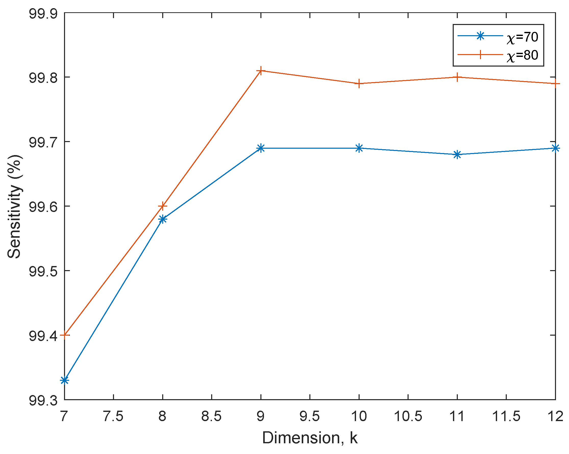
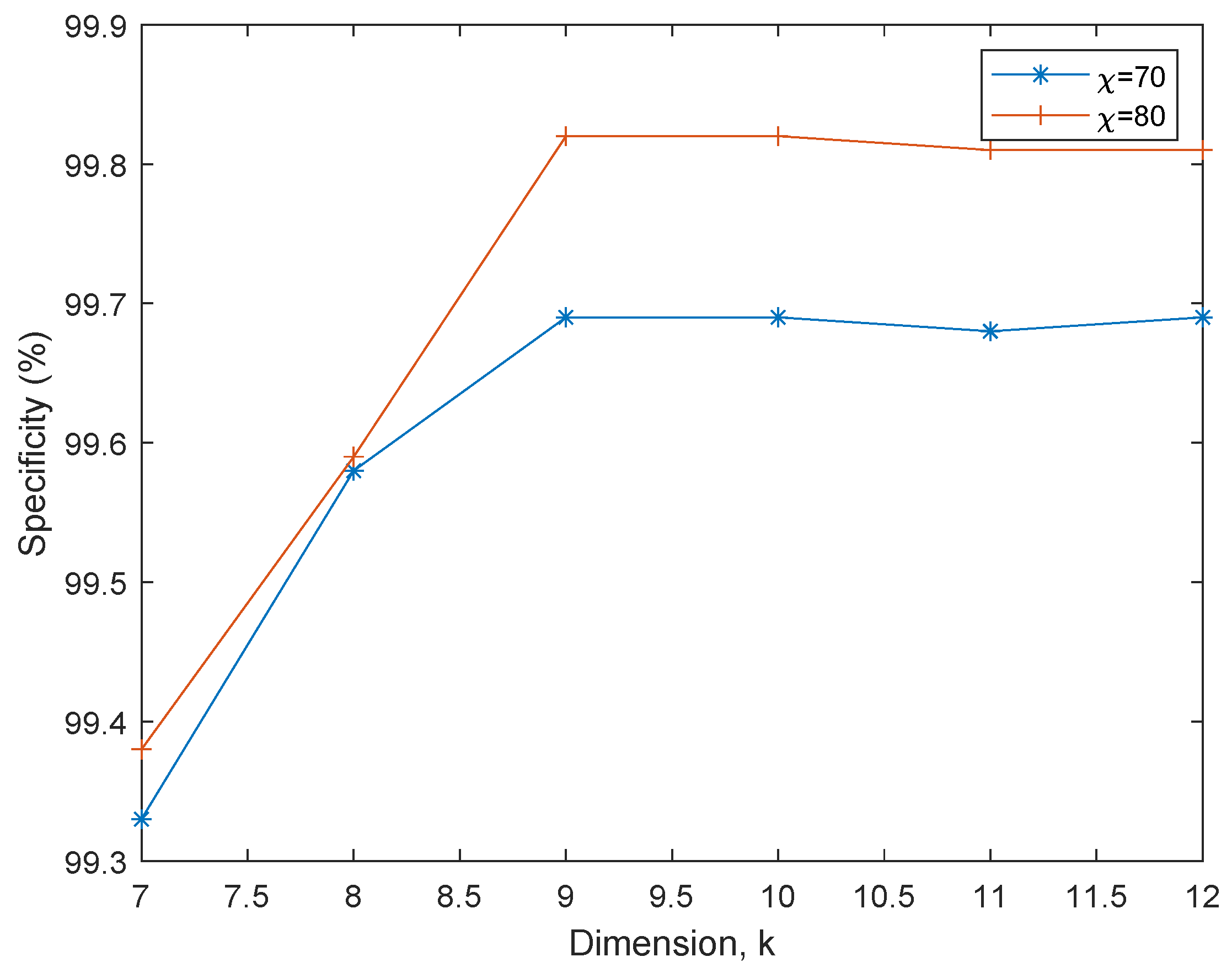
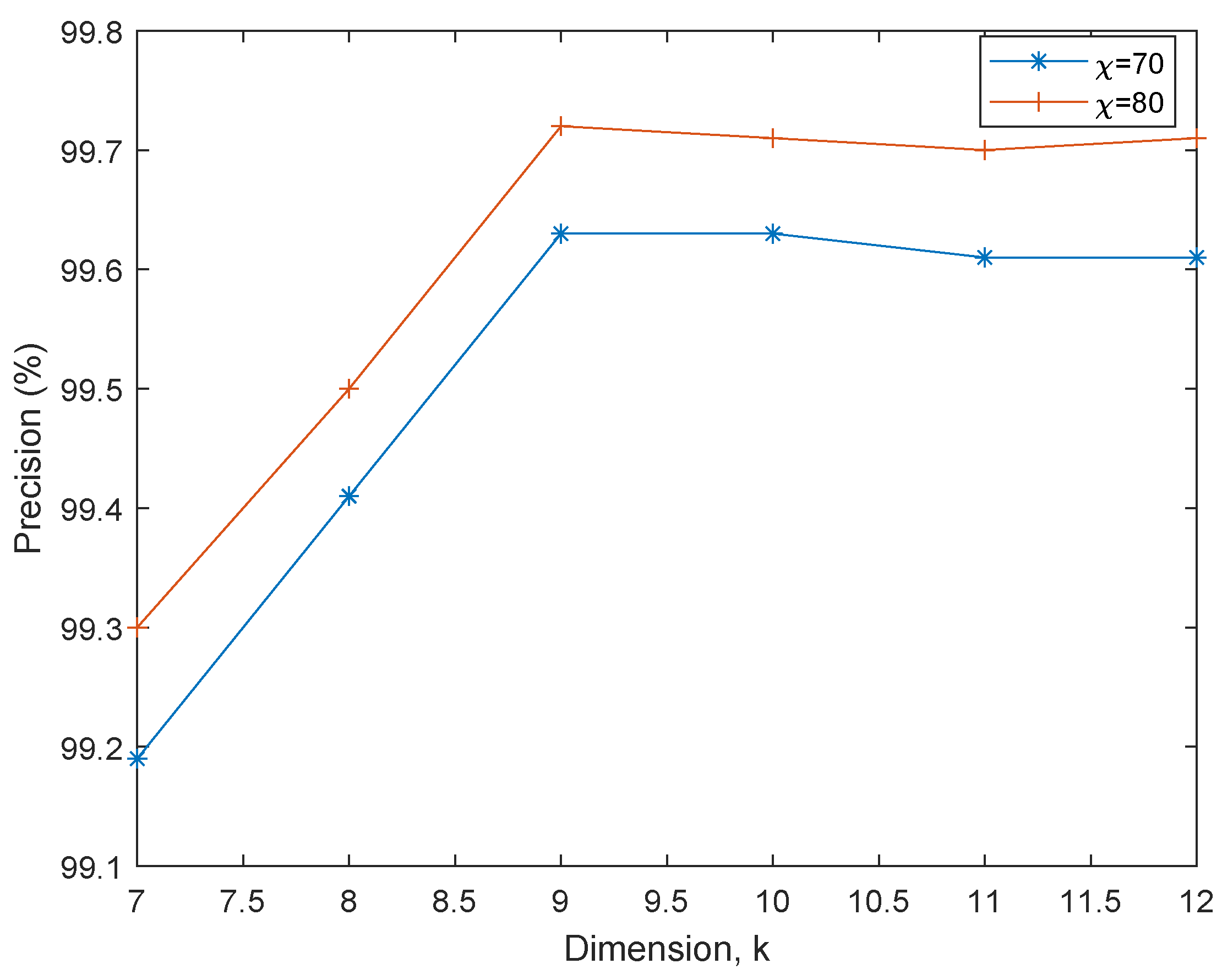
From Table 1, notice that the performance of the PCA-EHMM improves as the value of k increases from

k = 7 - 9

. For example, at

χ = 80

there is performance improvement of 0.20%, 0.21%, 0.20% and 0.21% in the

S_{e}

S_{p}

P

and

F 1

respectively as k increases from 7 to 8. Likewise, at

χ = 80

there is performance improvement of 0.21%, 0.23%, 0.22% and 0.22% in the

S_{e}

S_{p}

P

and

F 1

respectively as k increases from 8 to 9. Therefore, increasing the value of k does not result in a significant improvement in the prediction performance of the PCA-EHMM; instead, it increases the computing cost of the EHMM process. Thus,

k = 9

is chosen as the ideal number for k because it strikes a suitable compromise between performance gain and computational time complexity. Notwithstanding, this value of k is large enough to impose a high computational burden on the EHMM. As such, the MRE-EHMM is introduced in this article as discussed earlier.

To buttress, Figure 2, Figure 3, Figure 4 and Figure 5 depicts the PCA-EHMM performance as k rises in size. Notice how the curves of each figure flatten as k increases. This clearly shows that there are no significant increase in the performance of the PCA-EHMM, even if the entire derived principle components are used (that is,

d = 28

). Also, it is important to mention that the performance of the PCA-EHMM improves as the training size,

χ

increases from 70% to 80%. This performance improvement is evident in the four performance metrics considered.

6.3. MRE-EHMM Results and discussion

Table 1 shows the performance of the introduced MRE-EHMM in comparison to PCA-EHMM at

k = 9

. From the table, the MRE-EHMM and PCA-EHMM exhibited approximately the same

S_{e}

S_{p}

P

and

F 1

performances, even as

χ

increases. However, keep in mind that the MRE-EHMM is 5-dimensional while the PCA-EHMM is 9-dimensional. Whereas, the computational time complexity of the EHMM is proportional to the dimension size and increases as the dimension grows. Thus, when compared to the PCA approach, the MRE approach requires significantly less processing time from the EHMM. As a result, the MRE approach can be used as a more efficient performance alternative to the PCA approach for real-time credit fraud prediction systems.

Table 2. MRE-EHMM and PCA-EHMM performance comparison;

h = 5

and

k = 9

Table 2. MRE-EHMM and PCA-EHMM performance comparison;

h = 5

and

k = 9

$χ$ (%)	MRE-EHMM	PCA-EHMM	MRE-EHMM	PCA-EHMM	MRE-EHMM	PCA-EHMM	MRE-EHMM	PCA-EHMM
	$S_{e}$ (%)		$S_{p}$ (%)		$P$ (%)		$F 1$ (%)
70	99.68	99.69	99.70	99.70	99.62	99.63	88.69	99.70
75	99.80	99.79	99.80	99.82	99.72	99.71	99.80	99.80
80	99.81	99.81	99.81	99.82	99.73	99.72	99.81	99.82

7. Conclusion

This article analyses the performance of two feature extraction techniques that can be combined with the EHMM for the prediction of credit card fraud. The PCA method offered good performance in terms of the performance metrics considered. However, it exhibits a high computation burden on the entire prediction system. The MRE is introduced in the article as an efficient performance alternative to the PCA technique. Although the MRE technique offered the same

S_{e}

S_{p}

P

and

F 1

performances with the PCA technique, it exhibited significantly less processing time from the EHMM which makes it more suitable.

Author Contributions

O.O. and O.P. conceptualized the study. O.O., A.S., and O.M. completed the theoretical derivation, O.O. and O.P.established the model, carried out the simulation, and finished the writing of this manuscript. V. proofread and supervised the writing of the manuscript. The published version of the manuscript has been read and approved by all authors.

Funding

This research received no external funding.

Institutional Review Board Statement

Not applicable.

Informed Consent Statement

Not applicable.

Data Availability Statement

This study analyzed publicly available datasets. The data is available at https://www.kaggle.com/mlg-ulb/creditcardfraud (Accessed: 01 June 2023).

Conflicts of Interest

There are no conflicts of interest to be declared by the authors.

1	https://www.kaggle.com/mlg-ulb/creditcardfraud

References

Alkarkhi, A.F.M.; Alqaraghuli, W.A.A. Chapter 8 - Principal Components Analysis. In Easy Statistics for Food Science with R; Alkarkhi, A.F.M., Alqaraghuli, W.A.A., Eds.; Academic Press: London, UK, 2019; pp. 125–141. [Google Scholar]
Aristov, V.V.; Buchelnikov, A.S.; Nechipurenko, Y.D. The Use of the Statistical Entropy in Some New Approaches for the Description of Biosystems. Entropy 2022, 24, 172. [Google Scholar] [CrossRef]
Babalola, O.P.; Usman, A.M.; Ogundile, O.O.; Versfeld, D.J.J. Detection of Bryde’s Whale Short Pulse Calls using Time Domain Features with Hidden Markov Models. South African Institute of Electrical Engineers 2021, 112, 15–23. [Google Scholar] [CrossRef]
Baum, L.E.; Petrie, T.; Soules, G.; Weiss, N. A Maximization Technique Occurring in the Statistical Analysis of Probabilistic Functions of Markov Chains. Ann. Math. Statist. 1970, 41, 164–171. [Google Scholar] [CrossRef]
Bhasin, M.L. The Role of Technology in Combating Bank Frauds: Perspectives and Prospects. Ecoforum Journal 2016, 5, 200–212. [Google Scholar]
Dornadula, V.N.; Geetha, S. Credit Card Fraud Detection using Machine Learning Algorithms. Proc Comput Sci. 2019, 165, 631–641. [Google Scholar] [CrossRef]
Duda, R.; Hart, P.; Stork, D.G. Pattern Classification; 2nd ed.; Wiley: New York, NY, USA, 2001. [Google Scholar]
Fashoto, S.G.; Owolabi, O.; Adeleye, O.; Wandera, J. Hybrid Methods for Credit Card Fraud Detection Using K-means Clustering with Hidden Markov Model and Multilayer Perceptron Algorithm. Br. J. Appl. Sci. Technol. 2016, 13, 1–11. [Google Scholar] [CrossRef]
Forgy, E.W. Cluster Analysis of Multivariate Data: Efficiency versus Interpretability of Classification. Biometrics 1965, 21, 768–780. [Google Scholar]
Khan, A.; Singh, T.; Sinhal, A. Observation Probability in Hidden Markov Model for Credit Card Fraudulent Detection System. Proceedings of the Second International Conference on Soft Computing for Problem Solving (SocProS 2012) 2014, 236, 751–760. [Google Scholar] [CrossRef]
Khare, N.; Sait, S.Y. Credit Card Fraud Detection using Machine Learning Models and Collating Machine Learning Models. Int. J. Pure Appl. Math. 2018, 118, 825–837. [Google Scholar]
Ileberi, E.; Sun, Y.; Wang, Z. A Machine Learning Based Credit Card Fraud Detection using the GA Algorithm for Feature Selection. J. Big Data 2022, 9, 24. [Google Scholar] [CrossRef]
Iwasokun, G.B.; Omomule, T.G.; Akinyede, R.O. Encryption and Tokenization-Based System for Credit Card Information Security. Int. J. Cyber Secur. Digit. Forensics 2018, 7, 283–293. [Google Scholar] [CrossRef]
Lucas, Y.; Portier, P.-E.; Laporte, L.; He-Guelton, L.; Caelen, O.; Granitzer, M.; Calabretto, S. Towards Automated Feature Engineering for Credit Card Fraud Detection Using Multi-Perspective HMMs. Future Gener. Comput. Syst. 2020, 102, 393–402. [Google Scholar] [CrossRef]
MacQueen, J. Some Methods for Classification and Analysis of Multivariate Observations. In Proceedings of the Fifth Berkeley Symposium on Mathematical Statistics and Probability, Volume 1: Statistics; University of California Press: Berkeley, CA, USA; 1967; pp. 281–297. [Google Scholar]
Nalband, S.; Prince, A.; Agrawal, A. Entropy-Based Feature Extraction and Classification of Vibroarthographic Signal Using Complete Ensemble Empirical Mode Decomposition with Adaptive Noise. IET Sci. Meas. Technol. 2018, 12, 350–359. [Google Scholar] [CrossRef]
Ogundile, O.O.; Babalola, O.P.; Odeyemi, S.G.; Rufai, K.I. Hidden Markov Models for Detection of Mysticetes Vocalisations Based on Principal Component Analysis. Bioacoustics 2022, 31, 710–738. [Google Scholar] [CrossRef]
Ogundile, O.M.; Owoade, A.A.; Ogundile, O.O.; Babalola, O.P. Linear Discriminant Analysis Based Hidden Markov Model for Detection of Mysticetes’ Vocalisations. Sci. Afr. 2024, 24, e02128. [Google Scholar] [CrossRef]
Ogundile, O.O.; Usman, A.M.; Babalola, O.P.; Versfeld, D.J.J. Dynamic Mode Decomposition: A Feature Extraction Technique Based Hidden Markov Model for Detection of Mysticetes’ Vocalisations. Ecol. Inform. 2021, 63, 101306. [Google Scholar] [CrossRef]
Ogundile, O.O.; Usman, A.M.; Versfeld, D.J.J. An Empirical Mode Decomposition Based Hidden Markov Model Approach for Detection of Bryde’s Whale Pulse Calls. J. Acoust. Soc. Am. 2020, 147, EL125–EL131. [Google Scholar] [CrossRef] [PubMed]
Ogundile, O.O.; Usman, A.M.; Babalola, O.P.; Versfeld, D.J.J. A Hidden Markov Model with Selective Time Domain Feature Extraction to Detect Inshore Bryde’s Whale Short Pulse Calls. Ecol. Inform. 2020, 57, 101087. [Google Scholar] [CrossRef]
Ololade, B.M.; Salawu, M.K.; Adekanmi, A.D. E-Fraud in Nigerian Banks: Why and How? J. Financ. Risk Manag. 2020, 9, 211–228. [Google Scholar] [CrossRef]
Reynolds, D. Gaussian Mixture Models. In Encyclopedia of Biometrics; Li, S.Z., Jain, A., Eds.; Springer: Boston, MA, USA, 2009; pp. 659–663. [Google Scholar]
Richman, J.S.; Lake, D.E.; Moorman, J.R. Sample Entropy. In Numerical Computer Methods, Part E; Walker, J.M., Ed.; Academic Press: London, UK, 2004; Volume 384, pp. 172–184. [Google Scholar]
Robinson, W.N.; Aria, A. Sequential Fraud Detection for Prepaid Cards Using Hidden Markov Model Divergence. Expert Syst. Appl. 2018, 91, 235–251. [Google Scholar] [CrossRef]
Rushin, G.; Stancil, C.; Sun, S.; Adam, S.; Beling, P. Horse Race Analysis in Credit Card Fraud—Deep Learning, Logistic Regression, and Gradient Boosted Tree. In Proceedings of the 2017 Systems and Information Engineering Design Symposium (SIEDS); IEEE: New York, NY, USA, 2017; pp. 117–121. [Google Scholar]
Syms, C. Principal Components Analysis. In Encyclopedia of Ecology; Jørgensen, S.E., Fath, B.D., Eds.; Elsevier: London, UK, 2008; pp. 2940–2949. [Google Scholar]
Tharwat, A. Principal Component Analysis - A Tutorial. Int. J. Appl. Sci. Eng. 2009, 7, 41–61. [Google Scholar] [CrossRef]
Usman, A.M.; Ogundile, O.O.; Versfeld, D.J.J. Review of Automatic Detection and Classification Techniques for Cetacean Vocalization. IEEE Access 2020, 8, 105181–105206. [Google Scholar] [CrossRef]
Viterbi, A. Error Bounds for Convolutional Codes and an Asymptotically Optimum Decoding Algorithm. IEEE Trans. Inf. Theory 1967, 13, 260–269. [Google Scholar] [CrossRef]
Wang, X.; Wu, H.; Yi, Z. Research on Bank Anti-fraud Model Based on K-means and Hidden Markov Model. In Proceedings of the 2018 3rd IEEE International Conference on Image, Vision and Computing; IEEE: New York, NY, USA; 2018; pp. 780–784. [Google Scholar]
Xuan, S.; Liu, G.; Li, Z.; Zheng, L.; Wang, S.; Jiang, C. Random Forest for Credit Card Fraud Detection. In Proceedings of the 2018 IEEE 15th International Conference on Networking, Sensing and Control (ICNSC); IEEE: Zhuhai, China; 2018; pp. 1–6. [Google Scholar]

Figure 1. EHMM credit card prediction model

Figure 2. PCA-EHMM Sensitivity versus dimension performance

Figure 3. PCA-EHMM Specificity versus dimension performance

Figure 4. PCA-EHMM Precision versus dimension performance

Figure 5. PCA-EHMM F1-score versus dimension performance

Table 1. PCA-EHMM performance as a function of k.

$k = 7$
$χ$ (%)	$S_{e}$ (%)	$S_{p}$ (%)	$P$ (%)	$F 1$ (%)
70	99.33	99.27	99.19	99.30
75	99.39	99.39	99.31	99.39
80	99.40	99.38	99.30	99.39
$d = 8$
$χ$ (%)	$S_{e}$ (%)	$S_{p}$ (%)	$P$ (%)	$F 1$ (%)
70	99.58	99.49	99.41	99.54
75	99.60	99.61	99.52	99.61
80	99.60	99.59	99.50	99.60
$k = 9$
$χ$ (%)	$S_{e}$ (%)	$S_{p}$ (%)	$P$ (%)	$F 1$ (%)
70	99.69	99.70	99.63	99.70
75	99.79	99.82	99.71	99.80
80	99.81	99.82	99.72	99.82
$k = 10$
$χ$ (%)	$S_{e}$ (%)	$S_{p}$ (%)	$P$ (%)	$F 1$ (%)
70	99.69	99.71	99.63	99.70
75	99.80	99.81	99.70	99.81
80	99.79	99.82	99.71	99.81
$k = 11$
$χ$ (%)	$S_{e}$ (%)	$S_{p}$ (%)	$P$ (%)	$F 1$ (%)
70	99.68	99.70	99.61	99.69
75	99.79	99.79	99.71	99.79
80	99.80	99.81	99.70	99.81
$k = 12$
$χ$ (%)	$S_{e}$ (%)	$S_{p}$ (%)	$P$ (%)	$F 1$ (%)
70	99.69	99.71	99.61	99.70
75	99.79	99.80	99.72	99.80
80	99.79	99.81	99.71	99.80

Disclaimer/Publisher’s Note: The statements, opinions and data contained in all publications are solely those of the individual author(s) and contributor(s) and not of MDPI and/or the editor(s). MDPI and/or the editor(s) disclaim responsibility for any injury to people or property resulting from any ideas, methods, instructions or products referred to in the content.

© 2024 by the authors. Licensee MDPI, Basel, Switzerland. This article is an open access article distributed under the terms and conditions of the Creative Commons Attribution (CC BY) license (http://creativecommons.org/licenses/by/4.0/).

Copyright: This open access article is published under a Creative Commons CC BY 4.0 license, which permit the free download, distribution, and reuse, provided that the author and preprint are cited in any reuse.

MDPI Initiatives

Important Links

Choose an area of interest and we will send you notifications of new preprints at your preferred frequency.

Disclaimer

Credit Card Fraud: Analysis of Feature Extraction Techniques for Ensemble Hidden Markov Model Prediction Approach

Abstract

1. Introduction

2. Related Work

3. Dataset

4. Feature Extraction Techniques

4.1. Principal Component Analysis (PCA)

4.1.1. Standardisation

4.1.2. Covariance Matrix Computation, ∑

4.1.3. Eigenvector and Eigenvalues Computation

4.2. Statistical Features: MRE

4.2.1. Mean, M

4.2.2. Relative Amplitude, R

4.2.3. Entropy, E

5. Ensemble Hidden Markov Model (EHMM)

5.1. EHMM Training

6. Results and Discussion

6.1. Test Parameter

6.2. PCA-EHMM Results and Discussion

6.3. MRE-EHMM Results and discussion

7. Conclusion

Author Contributions

Funding

Institutional Review Board Statement

Informed Consent Statement

Data Availability Statement

Conflicts of Interest

References

MDPI Initiatives

Important Links

Subscribe

4.2.1. Mean, $M$