M-Learning: A Computationally Efficient Heuristic for Reinforcement Learning with Delayed Rewards

1. Introduction

The current development of artificial intelligence requires exhaustive computation [1], and the reinforcement learning (RL) area is no exception to this issue. Algorithms such as Deep Q-Network (DQN) [2] have achieved significant results in advancing RL by integrating neural networks. However, the requirement for thousands or millions of training episodes remains constant [3]. Training agents in parallel has proven to be an effective strategy [4] to reduce the number of episodes [5], which is feasible in simulated environments but poses an implementation challenge in real-world physical training environments.

In the context of reinforcement learning, Markov Decision Processes (MDPs) are typically the mathematical model used to describe the working environment [7]. MDPs have enabled the development of classical algorithms such as Value Iteration [8], Monte Carlo, SARSA, and Q-Learning, among others.

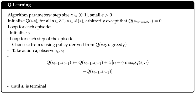
One of the algorithms most widely used is Q-Learning proposed by Christopher Watkins in 1989 [9]. Different approaches have been proposed based on the Q-Learning algorithm [10]. Its main advantage focuses on an optimal policy that maximizes the reward obtained by the agent if the action-state set is visited by a number infinitely many times [9]. The algorithm Q-Learning implemented in this work was taken from [9] and shown in Figure 1.

Some disadvantages of Q-Learning include the rapid table size growth as the number of states and actions [11] the problem of dimensional explosion. Furthermore, this algorithm tends to require a significant number of iterations to find a solution to a certain problem, and the adjustment of its multiple parameters can prolong this process.

Regarding the parameters of Q-Learning, the algorithm directly requires the assignment of the learning rate $\alpha$ and the discount factor $\gamma$, which are generally tuned empirically through trial and error by observing the rewards obtained in each training session [12]. The learning rate $\alpha$ directly influences the magnitude of updates made by the agent to its memory table. In [13], 8 different methods for tuning this parameter are explored, including iteration-dependent variations and changes based on positive or negative table fluctuation. Experimental results from [13] show that for the Frozen Lake environment, rewards converge above 10,000 iterations across all conducted experiments.

In Q-Learning, the exploration-exploitation dilemma is commonly addressed using the $ϵ$-Greedy policy, where one agent decides to choose between a random action and, the action with the highest Q-value with a certain probability. Current research around the algorithm focuses extensively on the exploration factor $ϵ$, as described in [14] and highlighted due to its potential to cause exploration imbalance and slow convergence [15,16,17].

The reward function significantly impacts the agent’s performance as reported in various applications. For instance, in path planning tasks for mobile robots [18], routing protocols in unmanned robotic networks [19], and scheduling of gantry workstation cells [20], the reward function plays a crucial role by influencing the observed variations in agent performance. Regarding the initial values of the Q-table, the algorithm does not provide recommendations for their assignment. Some works as [21], which utilize the whale optimization algorithm proposed in [22], aim to optimize the initial values of the Q-table to address the slow convergence caused by Q-Learning initialization issues.

The reward function directly impacts the agent’s training time. It can guide the agent through each state or be sparse across the state space, requiring the agent to learn from delayed rewards. As concluded in [23] when analyzing the effect of dense and sparse rewards in Q-Learning: "An important lesson here is that sparse rewards are indeed difficult to learn from, but not all dense rewards are equally good."

The heuristic proposed takes some conceptual ideas from Q-Learning along with its different proposals to search for alternatives focused on applications in real-physical environments. This heuristic allows for reducing the complexity of adjustment and time involved in the use of Q-learning. Moreover, the proposed algorithm, similar to Q-Learning, works on storage in a table and the relationship between states and actions through a numerical value. This algorithm is termed M-learning, and it will be explained in detail and referred to throughout the document.

2. Definition of the M-Learning Algorithm

The main idea for the M-learning approach is to reflect on how an agent is considered to solve a task and what this implies in terms of the elements that produce the Markov processes. In contrast to Q-learning, this is not defined directly, rather it is based on the premise that the proposed reward function is consistent to be achieved and that consequently, the agent will seek to maximize the reward by reaching to complete the task eventually. This perspective merges two different problems into the same element to tune: the reward function and the way to get the solution.

In general, in the formulation of a task or problem and presented, the solution is implicitly defined or vice versa, if a solution is described, the problem is implicit. Although there is no notion of how to get there, like two sides of a coin in which you cannot always notice both sides. On the other hand, if you are searching to control the angle in a dynamic system, the solution will be the position state to be ${\theta }_{ref}$. Now, when the approach of a task for an agent is thought within the framework of the MDP, the solution must also be described by its elements. Specifically, the solution to a task described as an MDP is a particular s of S, which we will call the objective state $s_g$.

In the reinforcement learning cycle, the reward signal aims to guide the agent in searching for a solution. Through it, the agent obtains feedback from the environment as to whether or not her actions are favorable. Q-learning uses a reward factor to modify the action-state and estimate its value. However, in environments where the reward is distributed dispersely and in which the agent most of the time does not receive feedback from the Q-learning environment, it must solve the search for the reward with time in exploration, reaching the exploitation-exploration dilemma, usually attacked with a policy of type $ϵ$-greedy.

The use of the $ϵ$-greedy policy, as a decision-making mechanism, requires the setting of the parameter of the decay rate ${ϵ}_d$, as the time that the agent will be able to explore looking for feedback from the environment, with a focus on reducing the number of iterations necessary to find a solution. This turns out to be decisive, as it is subject to the configuration before the training process and is not typical of the learning process, it is only possible to assign a favorable value by interacting with the problem through computation, making variations in the decay rate and number of iterations; keeping in mind that it is also conditioned by the rest of the parameters to be defined.

If the reward is thought of as the only source of stimulus for the agent in an environment with dispersed reward, the agent must explore the state space seeking to interact with states where it obtains a reward and, based on these, modify its behavior. As these states are visited more, the agent should be able to reduce the level of exploration and exploit more of its knowledge about the rewarded states. The agent explores in search of stimuli and to the extent that it acquires knowledge it also reduces arbitrary decision making. Exploration-exploitation can be understood discretely about each state in the state space. In this way, the agent can propose regions that it knows in the state space and, depending on how favorable or unfavorable, reinforce behaviors that lead it to achieve its objective or seek to explore other regions.

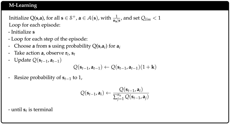
As stated, exploration and decision-making are strongly linked to the way the reward function is interpreted. The specific proposal in M-Learning consists of first limiting the reward function to values between -1 and 1, assigning the maximum value to the reward for reaching the goal state $s_g$. Second, each action in a state has a percentage value that represents the level of certainty about the favorableness of that action and, therefore, the sum of all actions in a state is 1. The M-Learning algorithm is shown below.

The first step in the M-Learning algorithm is the initialization of the table, unlike Q-learning, where the initial value can be set arbitrarily. The value of each state-action is initialized as a percentage value of the state according to the number of shares available. In this way, the initial value for each action of a state will be the same as shown in (1).

$$\begin{array}{cc}\hfill & \sum _{i=1}^{n_a}Q({\mathbf{s}}_j,{\mathbf{a}}_i)=1;\hfill \\ \hfill Q(s_j,a_i)& ={\displaystyle \frac{1}{n_a}};i=1,2,3,..,n_a\hfill \end{array}$$

(1)

Once the table is initialized, the cycle for the episodes begins; the initial state of the agreement agent is then established with observation of the environment. The cycle of steps begins within the episode and, based on the initial state of the agent, it chooses an action to take. To select an action, the agent evaluates the current state according to its table, obtains the values for each action, and it selects one at random using its value as its probability of choice. Thus, the value of each action represents its probability of choice for a given state, as presented in equation (2).

$$P\left({\mathbf{a}}_i\right|{\mathbf{s}}_j)=Q({\mathbf{s}}_j,{\mathbf{a}}_i)$$

(2)

After selecting an action, the agent acts on the environment and observes its response in the form of the reward and the new state. When the agent has already passed to the new state, evaluate the action taken and modifies the value of that action-state according to (3).

$$Q({\mathbf{s}}_{t-1},{\mathbf{a}}_{t-1})\leftarrow Q({\mathbf{s}}_{t-1},{\mathbf{a}}_{t-1})(1+\mathbf{k})$$

(3)

The percentage value of modification $\mathbf{k}$ of the value of the previous state-action $s_{t-1}$ is computed under the existence consideration of the reward (4), if ${\mathbf{r}}_t$, exists, $\mathbf{k}$ is calculated based on the current reward or the current and previous reward. If there is no reward stimulus, it is calculated as the differential of information contained in the current state and previous $\Delta I$.

$$K=\left\{\begin{array}{ccc}{f}_r\hfill & si& |r_t|\ne 0\\ \\ \Delta I\hfill & si& r_t=0\end{array}\right.$$

(4)

When the environment returns a reward to the agent for his action, $|r_t|\ne 0$, $r_t$ is a measure of the approach or distance concerning $s_g$, , in specific, the best case of the new state will be the target state $s_t=s_g$ with maximum positive reward $r_t=1$, in the other case, the new state will be a state radically opposite to the objective state and its reward will be maximum but negative $r_t=-1$. For cases where the reward is not maximal, the value of $f_r$ may be calculated by a function that maps the reward differential within the range of $[-1,1]$, for this case, a first-order relation is proposed.

$$f_r=\left\{\begin{array}{ccc}{r}_t\hfill & si& |r_t|=1\\ \\ {\displaystyle \frac{r_t-r_{t-1}}{2}}\hfill & si& 0<|r_t|<1\end{array}\right.$$

(5)

If the reward function of the environment is described inform such that its possible values are 1, 0, and -1; the calculation of k can be rewritten by replacing $f_r$ with $r_t$. This representsenvironments where it is difficult to establish a continuous signal that correctly guides the agent through the state space to reach your goal. In these situations, it may be convenient to only generate a stimulus on the agent by achieving the objective or cause the end of the episode. According to this, the Equation (4) can be rewritten as (6).

$$K=\left\{\begin{array}{ccc}{r}_t\hfill & si& |r_t|\ne 0\\ \\ \Delta I\hfill & si& r_t=0\end{array}\right.$$

(6)

When the environment does not return a reward $r_t=0$, the agent evaluates the correctness of its action based on the difference in information stored for its current and previous state, as depicted in Equation (7). This is the way the agent spreads the reward stimulus.

$$\Delta I=I\left(s_t\right)-I\left(s_{t-1}\right)$$

(7)

To calculate the information of a state $s_j$, the difference between the value of the maximum action and the average of the possible actions in that state is evaluated in Eq. (8). The average value of the stock is also its initial value, which represents that there is no knowledge in that state that the agent can use to select a stock. In other words, the variation concerning the mean is a percentage indicator of the level of certainty that the agent has in selecting a certain action.

$$I\left(s_j\right)=max\left(s_j\right)-{\displaystyle \frac{1}{n_a|s_j}}$$

(8)

Since the number of shares available for the previous and current state may be different, which modifies the average value of the shares, it is necessary to put them on the same scale to be able to compare them. When the average value of the shares is established, its maximum variation of information is also established, this is how much is needed in the value of an action to have a probability of 1. The maximum information is then the difference between the maximum value and the average share value (9).

$$Ima{x}_{s_j}=1-{\displaystyle \frac{1}{n_a|s_t}}$$

(9)

Since we want to modify the previous state-action, we adjust the information value of the current state to the information scale of the previous state, using (10).

$$I^{\prime }\left(s_t\right)=I\left(s_t\right){\displaystyle \frac{Ima{x}_{s_{t-1}}}{Ima{x}_{s_t}}}$$

(10)

It is possible that for a state $s_t$ all its actions have been restricted in such a way that the value of all its shares possible is zero making it impossible to calculate the maximum information of $s_t$. For this reason, a negative constant value is established to indicate that the action taken leads to a state that we want to avoid. With this, the information differential is defined according to (7).

$$\Delta I=\left\{\begin{array}{ccc}{I}^{\prime }\left(s_t\right)-I\left(s_{t-1}\right)\hfill & si& \sum _{i=1}^{n_a}Q({\mathbf{s}}_t,{\mathbf{a}}_i)=1\\ \\ -Q_{lim}\hfill & si& \sum _{i=1}^{n_a}Q({\mathbf{s}}_t,{\mathbf{a}}_i)=0\end{array}\right.$$

(11)

The magnitude $Q_{lim}$ is a parameter that controls the level of maximum saturation of an action due to propagation. With this value, it is possible to control how close the value of an action can be to the possible extremes 0 and 1.

After calculating k and making the modification in the action-state $Q({\mathbf{s}}_{t-1},{\mathbf{a}}_{t-1})\leftarrow Q({\mathbf{s}}_{t-1},{\mathbf{a}}_{t-1})(1+\mathbf{k})$ must be distributed the probabilities within the state to maintain ${\sum }_{i=1}^{n_a}Q({\mathbf{s}}_{t-1},{\mathbf{a}}_i)=1$ applying (12) for state actions previous.

$$a_i^{\prime }={\displaystyle \frac{a_i}{{\sum }_{i=1}^{n_a}Q({\mathbf{s}}_{t-1},{\mathbf{a}}_i)}}i=1,2,3,..,a_n|s_{t-1}$$

(12)

In this way the variation in the value of the selected action over the rest of the actions. The beginning What is established is that the agent, having greater certainty of an action, reduces the possibility of selection of the other actions, or, on the contrary, by reducing the possibility of selecting an action, increases the level of certainty about the rest of the actions.

Similar to the $ϵ$-greedy, if you want to maintain a level minimum exploration value, it is necessary to restrict the maximum value that an action can achieve. This is established by the parameter $Q_{lim}$,, by conditioning the calculation of the redistribution of probabilities for the case in which the maximum action exceeds the saturation limit; ; $max\left(s_{t-1}\right)>Q_{lim}$, if this happens, it reduces the value of $max\left(s_{t-1}\right)$ in such a way that when applying (12) it becomes the saturation limit $Q_{lim}$.

$$ma{x}^{\prime }\left(s_{t-1}\right)={\displaystyle \frac{Q_{lim}}{1-Q_{lim}}}\sum _{i=1}^{n_a}Q({\mathbf{s}}_{t-1},{\mathbf{a}}_i)-max\left(s_{t-1}\right)$$

(13)

Finally, we return to the beginning of the cycle for the number of steps and continue executing the algorithm until reaching the limit of steps or reaching a final state.

3. Experimental Setup

In order to compare the performance of M-Learningagent training is carried out in front of Q-Learning using both algorithms in two different environments. Both groups of agents will have the same number of episodes of training and the same step limit per episode.

To measure the performance of the agents, a test is carried out Finish each episode until you complete the episode limit. During the episode, the agent will be able to modify his table according to her algorithm. At the end of the episode, either by reaching an end state or reaching the limit of steps per episode, The agent goes to the test stage where it cannot modify the values from her table. In the test stage, the agent plays 100 episodes with the table obtained at the end of the episode training. The policy applied in both agents for theselecting an action in the test is always taking the action with a higher $max\left(s\right)$ value. In this way, we seek to measure the agent’s learning process and its ability to maintain the knowledge acquired.

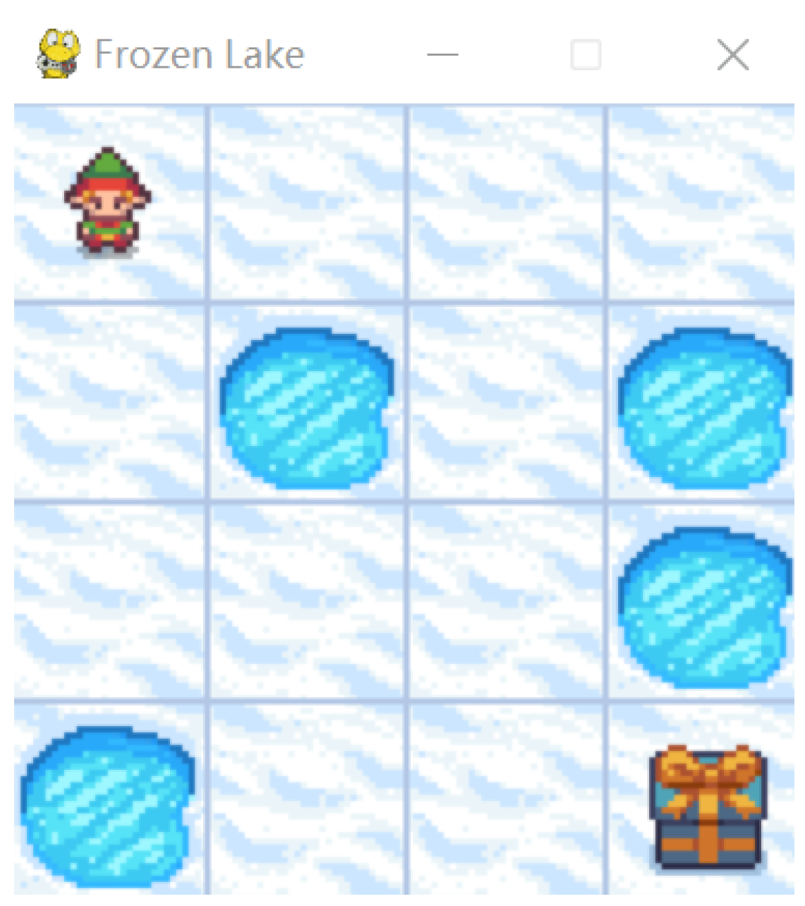
The selected environment is Frozen Lake, Figure 1, which It consists of crossing a frozen lake without falling through a hole. Frozen Lake is available at the Gymnasium bookstore, which is a maintained fork of OpenAI’s Gym [24] library which they define as ”An API standard for learning for reinforcement.” This environment has two variations which represent two different problems for the agent, In the first case, the environment allows the agent to move in the desired direction, and the state transition function of the environment is deterministic; In the second case when the agent wants to move in a certain direction environment may or may not lead you in that direction with a certain probability, the state transition function of the environment It is stochastic.

In the Frozen Lake environment, the agent receives a reward of 1 for reaching the other end of the lake, -1 for falling into a hole, and 0 for the rest of the states. For the stochastic environment, the agent will move in the desired direction with a probability of 1/3; otherwise, it will move in any direction perpendicular with the same probability of 1/3 in both directions. Table 1 summarizes the configuration of the experimental methodology.

3.1. Parameter Tuning

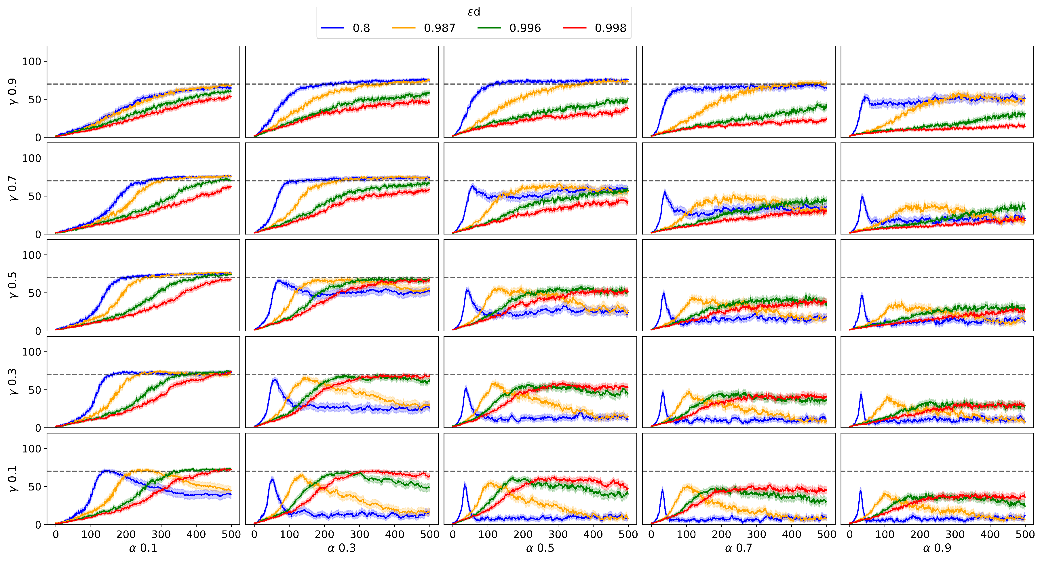
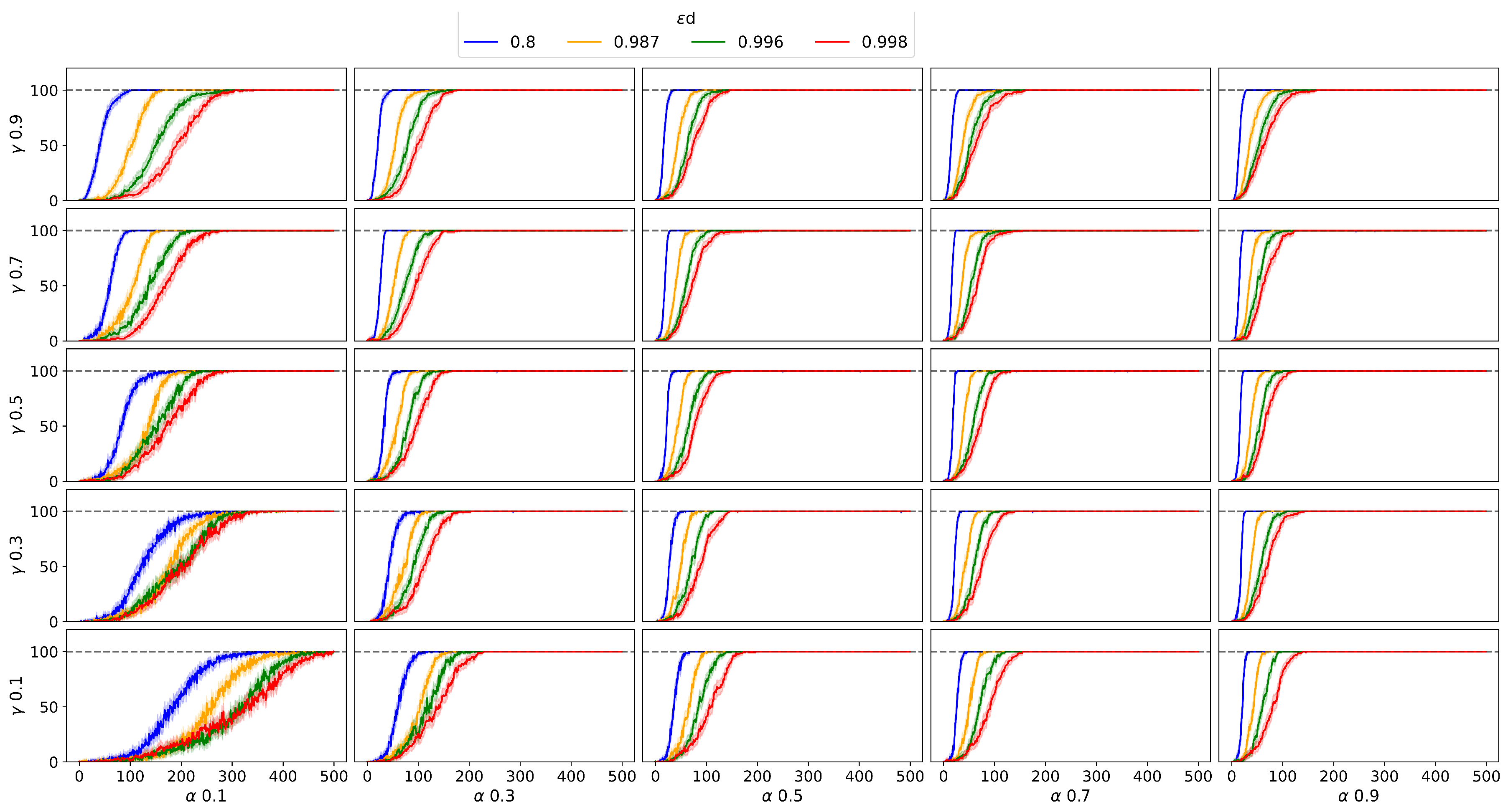
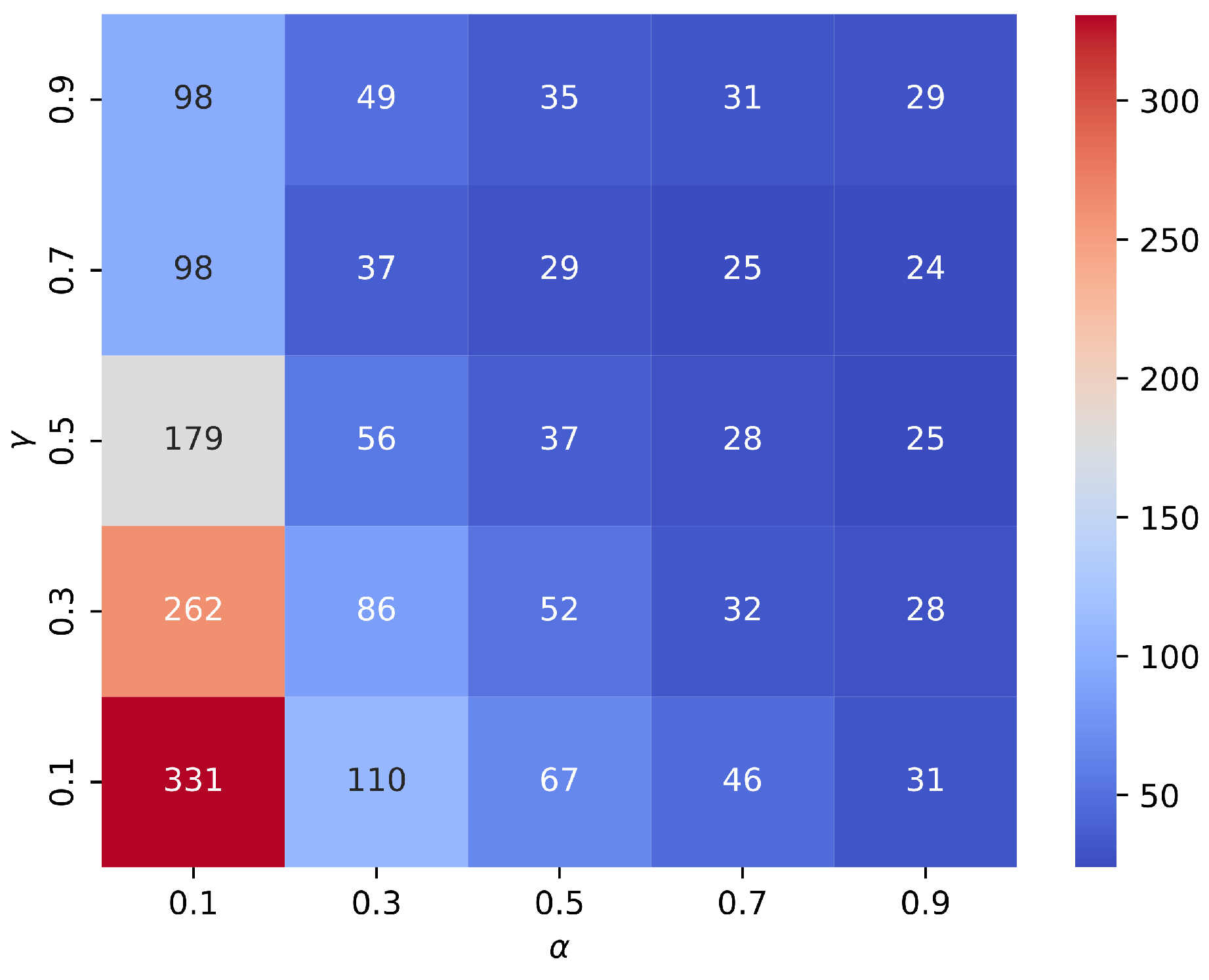
To train agents using Q-Learning it is necessary to set the parameters of the algorithm. The initial values of the table are set as a pseudo-random value from 0 to 1. The value of ${ϵ}_{min}$ for the $ϵ$-greedy policy is set to 0.005. Since $\alpha$, $\gamma$ and ${ϵ}_d$ directly impact the performance of the algorithm, a mesh search is performed for these 3 parameters.

• ${ϵ}_d$: 0.8, 0.987, 0.996, 0.998
• $\alpha$: 0.1, 0.3, 0.5, 0.7, 0.9
• $\gamma$: 0.1, 0.3, 0.5, 0.7, 0.9

The training of agents using our proposed M-learning method requires the setting of $Q_{lim}=0.96$ parameter.

4. Results

A set of data is obtained with the scores of each agent to the test carried out after every episode. For each particular test, there are 200 scores per episode, for each episode the value is averaged of the scores and also their 95% confidence interval, assuming a normal distribution. The results obtained are displayed as line graphs, plotting the average value in a strong color and the confidence interval as the area around the solid line with a stronger color faint.

4.1. Deterministic Environment

4.1.1. Q-Learning

Figure 2 shows the results for the agents trained with the Q-Learning algorithm and the grid-search of its paramters. In specific, the results presented by 20,000 agents in the Frozen Environment Deterministic Lake are reported. The main observation was the increase of the ${ϵ}_d$, which is equivalent to the increase in exploration time, it causes agents to require more episodes to find a policy capable of solving $100\%$ of the tests. The smaller values of $\alpha$ increase the dispersion in the agent scores and the increase in $\gamma$ reduces the time it takes for agents to achieve the goal, 100 times the test.

The criterion for selecting a set of parameters as the best, it is proposed to take the combination with the least number of episodes required for its average value to Achieve 100% of the test tests. Based on this criterion, shown in Table 2 the results for ${ϵ}_d=0.8$ are ordered from largest to smallest.

Figure 3 shows the behavior of the exploration inmesh for ${ϵ}_d=0.8$ according to the proposed criterion. It is noted how the best results are located in the value region high for parameters $\alpha$ and $\gamma$.

The best set of parameters corresponds to $\alpha$: 0.9, $\gamma$: 0.7, ${ϵ}_d$: 0.8, where the average of the agents trained with Q-Learning obtained a score of 100 for the test in episode 24. Figure 4 shows the training result of 1000 agents, using the best set of parameters, together with its standard deviation per episode. By increasing the number of agents, with the same set of parameters, Q-Learning obtained a score of 100 for the test in episode 26 for all agents.

Figure 4. Set of parameters with the lowest number of episodes to achieve a score of 100 in the test.

Figure 4. Set of parameters with the lowest number of episodes to achieve a score of 100 in the test.

Figure 5. Q-Agents results stochastic environment.

Figure 5. Q-Agents results stochastic environment.

4.1.2. M-Learning

Figure 6 shows the results obtained per 1000 agents trained with the M-Learning algorithm in the environment Frozen Lake deterministic. It can be seen how, during the 500 episodes, the average groups the behavior of the 1000 agents. The average score reaches $100\%$ of the test in episode 18, the standard deviation is also included per episode of results.

4.2. Stochastic Environment

4.2.1. Q-Learning

In Figure 5 shows the results obtained for the agents trained with Q-learning and the grid search of its parameters. In total, the results obtained by 20000 agents in the stochastic Frozen Lake environment are shown. It can be seen that the increase in ${ϵ}_d$ increases the exploration time, this causes the agents to require more episodes to find a stable policy. Unlike deterministic Frozen Lake, it is not possible to achieve $100\%$ of test tests due to the nature of the environment.

As a criterion for selecting a set of parameters, two conditions are proposed: the first, taking the combination with the lowest number of episodes required so that its average value exceeds $70\%$ of the test tests, and the second, that during the rest of episodes, its average is not below 65. Based on this criterion, the results that meet the first condition are displayed in the Table 3 ordered from highest to lowest.

The best set of parameters corresponds to $\alpha$: 0.3, $\gamma$: 0.7, ${ϵ}_d$: 0.8, where the average of the agents trained with Q-Learning obtained a higher score to 70 for the test in episode 101. Figure 7 shows the training result of 1000 agents, using the best set of parameters, along with their standard deviation per episode. By increasing the number of agents, with the same set of parameters, Q-Learning obtained a score above 70 for the test in episode 120.

4.2.2. M-Learning

In Figure 8 presented the results obtained by 1000 agents trained with the M-Learning algorithm in the stochastic Frozen Lake environment. It can be seen how during the 500 episodes the average groups the behavior of the 1000 agents, the average score exceeds the $70\%$ of the test in episode 46, and the standard deviation per episode of the results is also included.

5. Discussion

5.1. Deterministic Environment

In Figure 9 presents the best solutions obtained by the agents trained with Q-Learning and M-Learning, along with their standard deviations per episode. It can be seen how M-Learning first reaches the score of 100 with a smaller standard deviation area than Q-Learning. It can also be seen that Q-Learning, by continuing the learning process, may at some point have losses in the acquired knowledge and present a score less than 100, even when the environment remains the same.

The frequency with which the agents achieve the objective for each episode may be analyzed, based on the evaluation criterion and the episode where the agents achieve it. This is shown in Figure 10, which illustrates the number of agents who achieved a score of 100 on the test in each episode.

The agents trained with Q-Learning achieved the goal on average in episode 13,827 with a standard deviation of 4.18 episodes, while the agents trained with M-Learning took an average of 12,456 episodes to reach the goal, with a standard deviation of 1.74 episodes. This represents a $9.91\%$ reduction in the average number of episodes needed to achieve the goal and a $58.37\%$ reduction in the standard deviation of episodes from the mean.

5.2. Stochastic Environment

In Figure 11 shows the best solutions obtained by the agents trained with Q-Learning and M-Learning, along with their standard deviations.

It can be seen how M-Learning first surpasses the score of 70 with a smaller standard deviation area than Q-Learning. It can also be seen that Q-Learning, by continuing the learning process, converges with a higher standard deviation than M-Learning.

In Figure 12 attention is focused on the evaluation criterion and the episode where the agents reach it. For each episode, the number of agents who achieved a score greater than 70 in the test is depicted.

The agents trained with Q-Learning achieved the objective on average in episode 57,591, with a standard deviation of 14.77 episodes, while the agents trained with M-Learning took 31,186 episodes on average to achieve the objective with a standard deviation of 7.42 episodes, reducing the average number of episodes to achieve the objective by $45.84\%$ and the standard deviation of episodes concerning the mean by $49.75\%$.

6. Conclusions

The use of reinforcement learning for an unknown problem using Q-Learning, requires carrying out a broad exploration of its parameters, as presented in Figure 2 and Figure 5, with very diverse results and in some cases, non-convergence to a solution. This undoubtedly entails computing multiple times or making a systematic exploration with different parameters in the same environment. In this work, a total training of 42,000 agents was carried out, and 21,000,000 episodes with Q-Learning; before 2,000 agents and 1,000,000 M-Learning episodes.

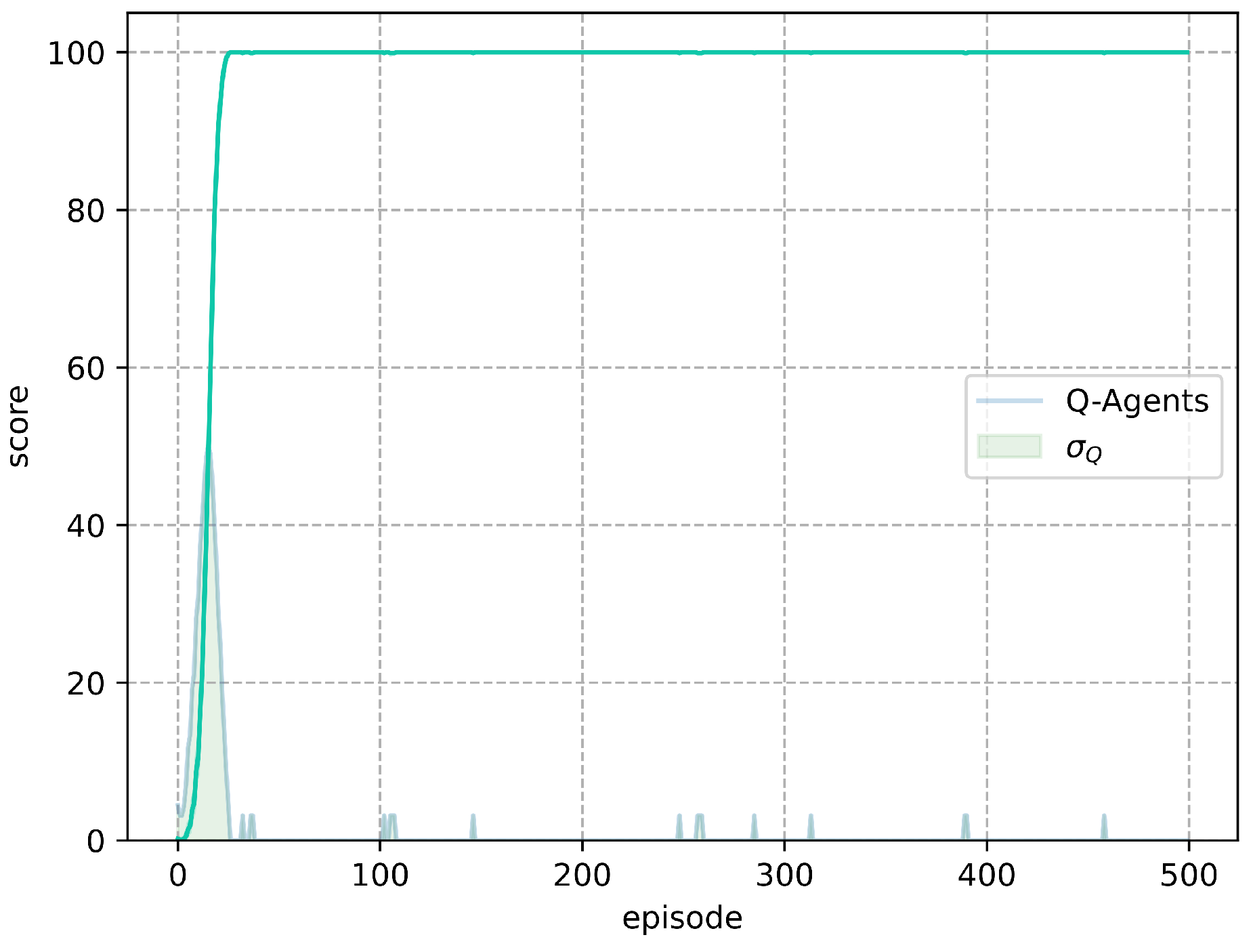
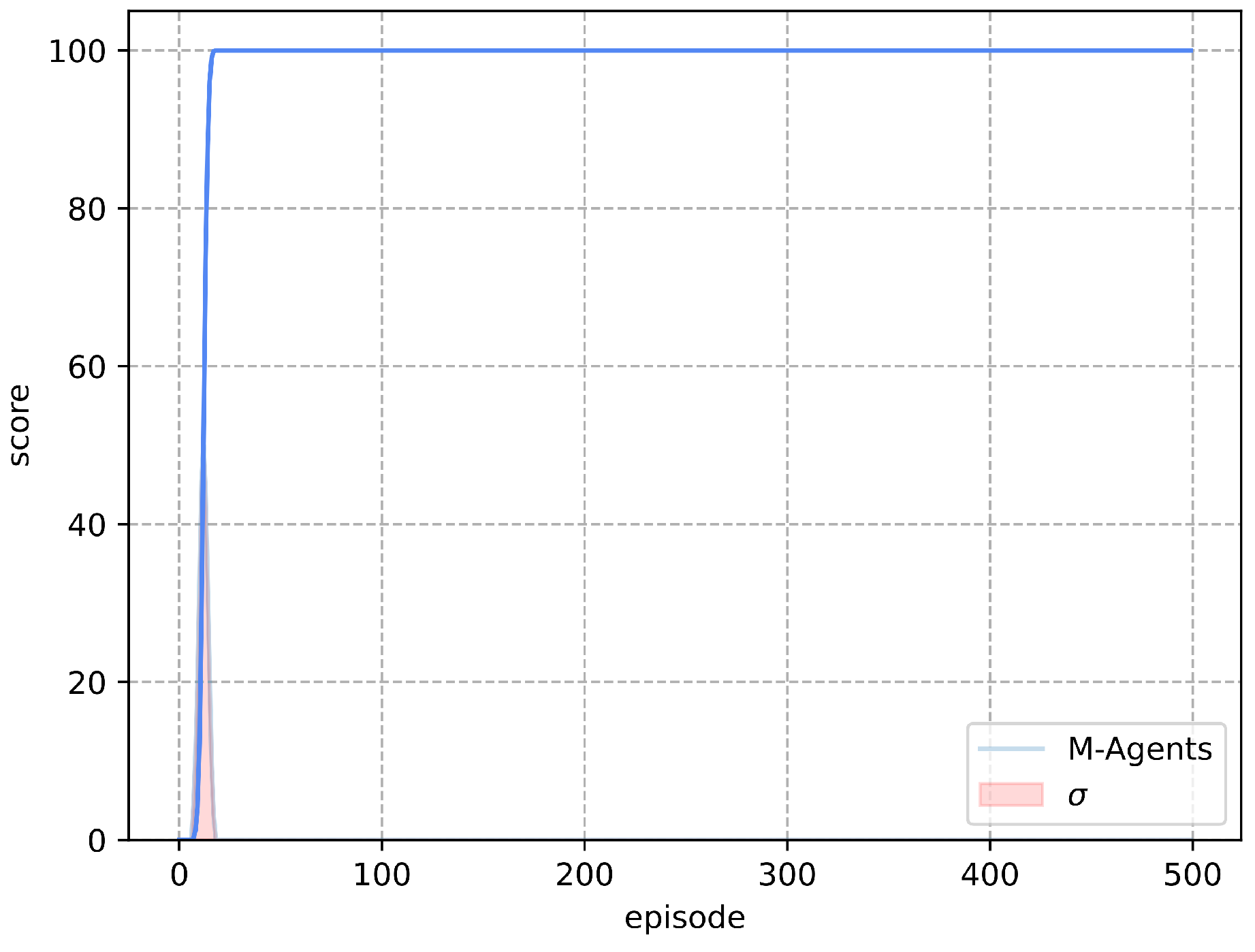
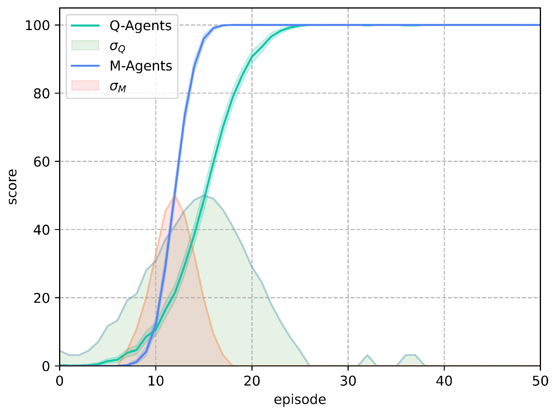
For the Frozen Lake environment deterministic, the algorithm M-Learning shows faster learning with less variability in the results obtained by the trained agents compared to Q-Learning as presented in Figure 9. M-Learning takes 8 episodes less than Q-Learning for all agents to achieve score of 100 for the deterministic configuration of the environment. This represents a decrease of 30.7% in the number of episodes necessary for all agents to achieve a score of 100. 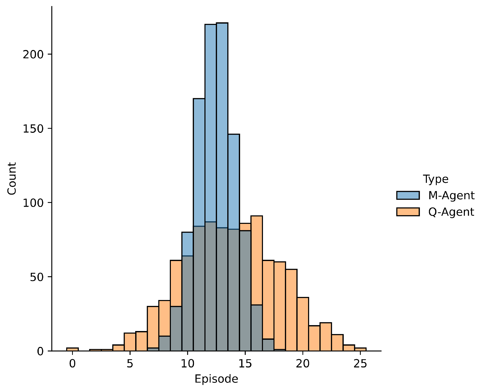Regarding the way in which the results obtained are distributed, Figure 10, although the average number of episodes to achieve the objective among the two algorithms have a difference close to one episode; M-learning presents a reduction of 58.37% in the standard deviation of episodes, which shows more consistent results.

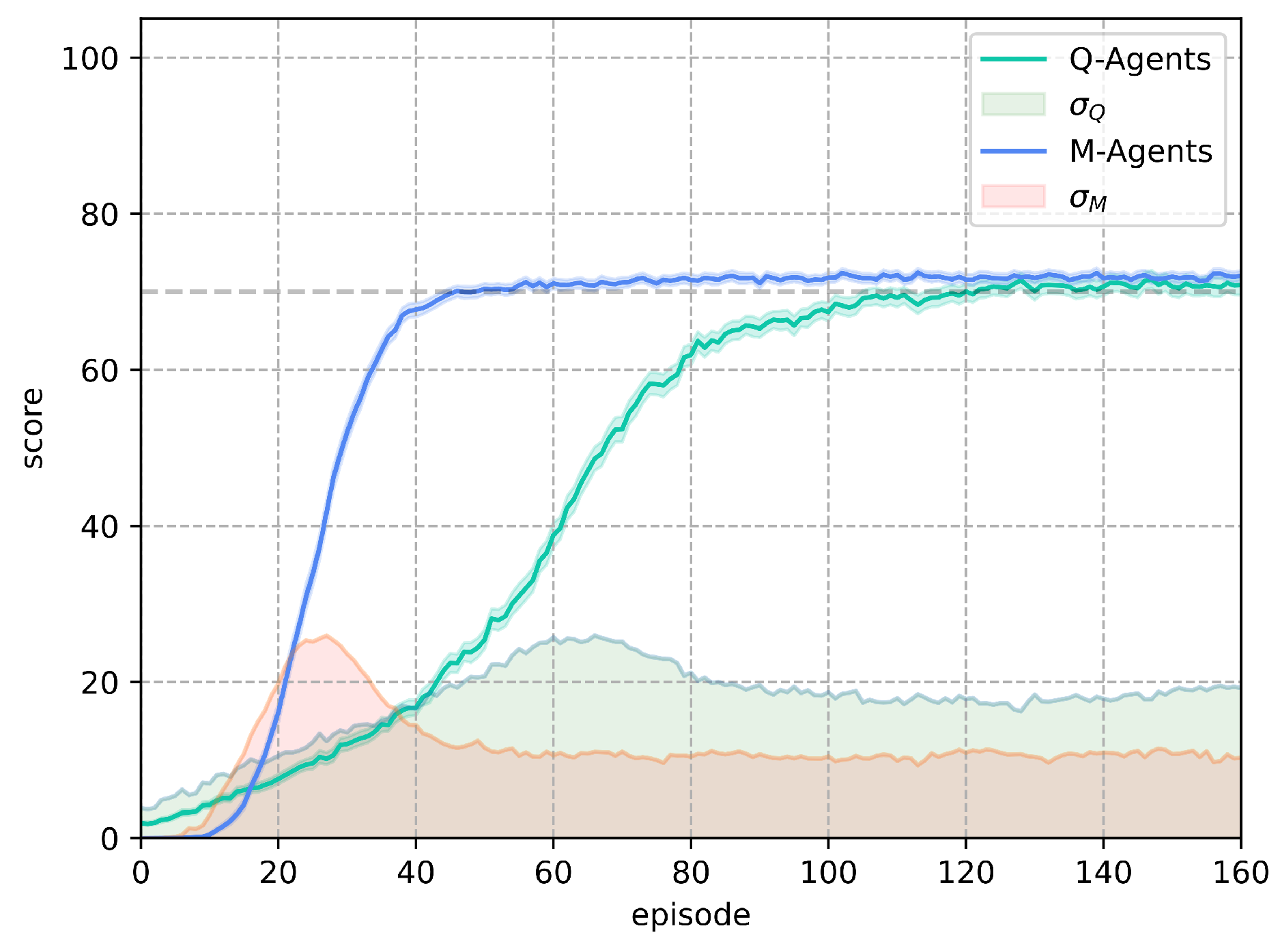
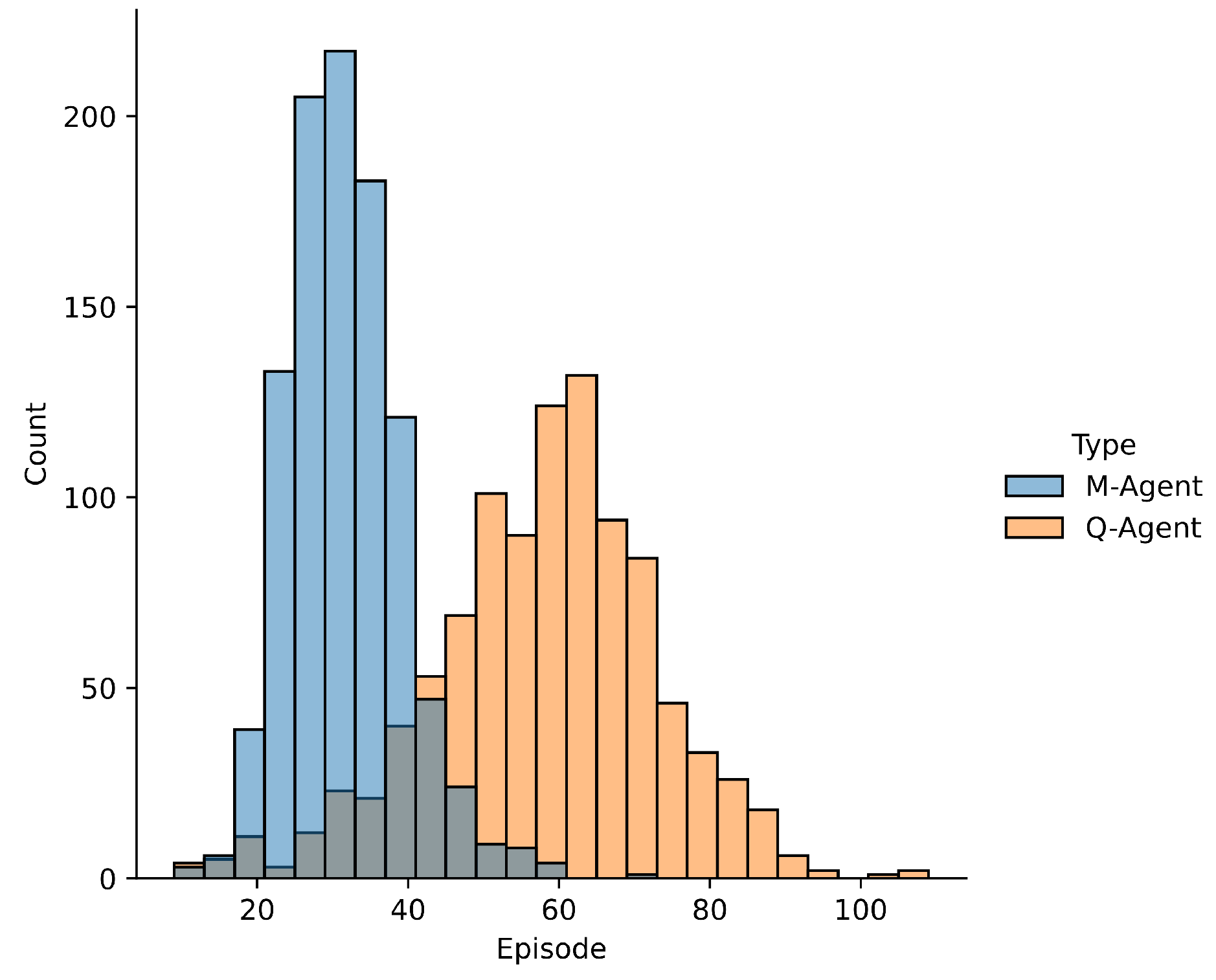
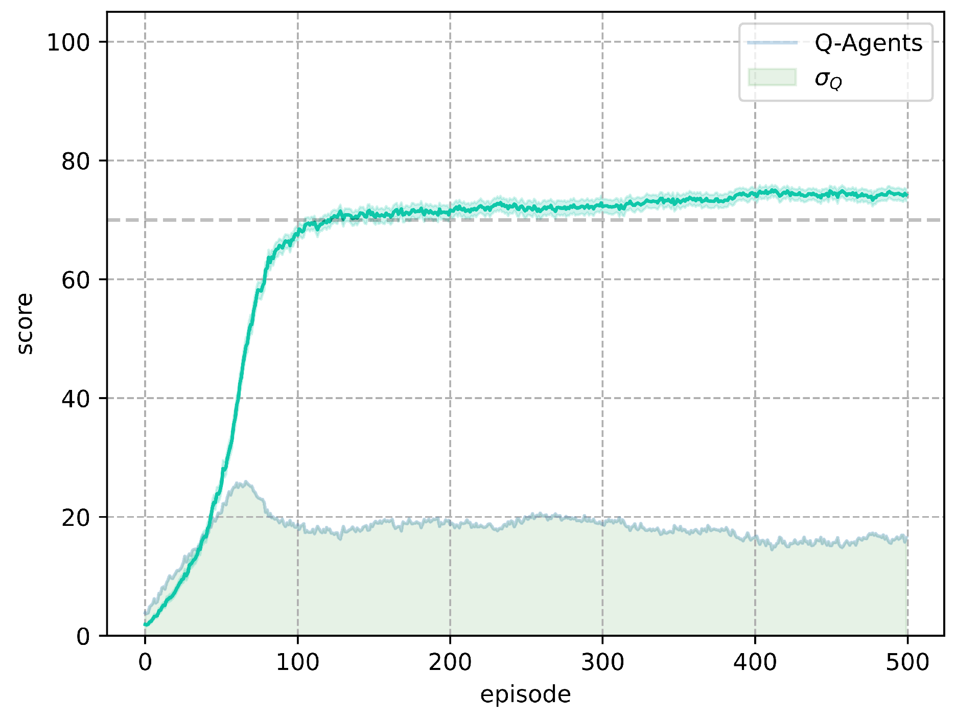
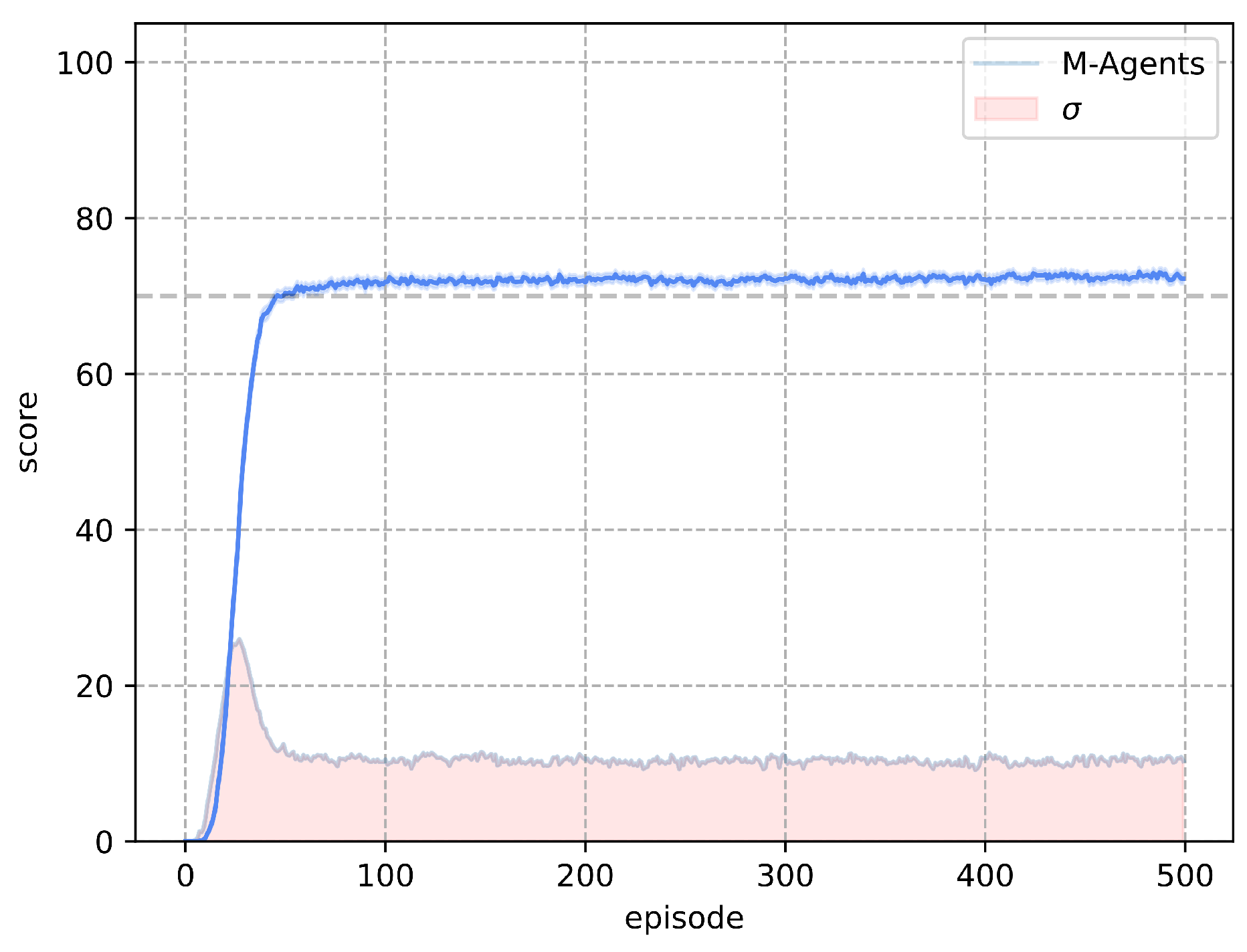
For the stochastic Frozen Lake environment, the algorithm M-Learning shows faster learning with less variability in the results obtained by the trained agents compared to Q-Learning as presented in Figure 11. M-Learning takes 74 episodes less than Q-Learning to obtain a score above 70 for all agents in the stochastic configuration of the atmosphere. This represents a decrease of 61.66% in the number of episodes necessary for all agents to exceed a score of 70. Regarding how the results obtained are distributed, in Figure 12, the average number of episodes to achieve the objective is 45.84%. lower for M-Learning, similar to the deterministic environment M-Learning presents a reduction of 49.75% in the standard deviation of episodes, which shows more consistent results.

Finally, for the Frozen Lake environment in its two configurations and with delayed reward, the algorithm proposed M-Learning with a single parameter to tune $Q_{lim}$, presents better performance with a smaller number of episodes and less variability in the scores of the agents. The results obtained in this document show that the proposed heuristic for the propagation of the information with delayed reward is favorable for environments like Frozen Lake.

With the results obtained for M-Learning, it is proposed That future research continue with the evaluation of its behavior in other environments, to identify the problems where it can be useful.