
Submitted:
13 September 2024
Posted:
15 September 2024
You are already at the latest version
Abstract
The success of deep learning (DL) in offline brain-computer interfaces (BCIs) has not yet translated into efficient online applications. This is due to three primary challenges. First, most DL solutions are designed for offline decoding, making the transition to online decoding complex and unclear. Second, the use of sliding windows in online decoding increases the computational complexity of DL training. Third, DL models typically require large amounts of training data, which are often scarce in BCI applications. To address these issues and enable real-time decoding, even across different subjects without calibration data, we first introduce a novel approach called real-time adaptive pooling (RAP). RAP modifies the pooling layers of existing offline DL models towards the online decoding requirements. Additionally, it significantly reduces the computational demand during training by jointly decoding consecutive windows. To reduce the amount of training data required, our approach leverages different levels of domain adaptation. We show how different settings enable different adaptation solutions. The results demonstrate that our approach is both powerful and can be calibration-free, providing a robust and practical solution for real-time BCI applications. These findings pave the way for the development of co-adaptive and highly efficient DL-based online BCI systems.
Keywords:
Motor imagery
; Electroencephalography
; Deep Learning
; Online decoding
; Domain adaptation
; Calibration-free
; Mutual learning
1. Introduction
Brain-computer interfaces (BCIs) enable direct communication between the human brain and external devices. As technology advances, the range of applications for BCIs spans from medical rehabilitation to enhancing human-computer interaction and entertainment [1]. One common method to control a BCI is through the motor imagery (MI) paradigm. MI BCIs are particularly utilized as a rehabilitation strategy for post-stroke patients, helping in the recovery of affected limbs [2,3]. During MI the user imagines the movement of a body part without actual physical execution. This process of imagination shares neural mechanisms with the actual execution [4], which makes MI BCIs especially suited for motor recovery in chronic stroke patients. Specifically, during MI, the power of the and rhythm measured over the sensorimotor area of the brain decreases (event related de-synchronization) and recovers after MI (event related synchronization).
BCIs in general, but especially MI BCIs are (initially) difficult to operate for inexperienced users as they rely on the endogenous modulation of brain rhythms [5] instead of external stimuli. Consequently, a large percentage of users is not able to control a BCI, a problem known as BCI inefficiency [6,7]. [6] and [7] split BCI users into different groups based on their performances and recommend different solutions for each group to improve their performance. These recommendations include longer/better user training, using a better decoder (which is able to extract more complex features) and employing adaptive decoders to circumvent distribution shifts.
User learning is particularly important as there are users that exhibit promising brain modulation during the initial screening but then fail to elicit the proper signals during MI [7]. In other words, among the users who are categorized as inefficient, there are users which have the potential to efficiently control a BCI, which marks a lost opportunity if not addressed appropriately. Encouragingly, research indicates that BCI usage is a learnable skill [8,9,10,11,12,13] where users are able to improve their performance and brain modulation [14] through longitudinal training. A crucial part of learning or mastering any skill is the guidance and feedback received during or after the execution [15]. BCIs that provide feedback to the user are referred to as closed-loop or online BCIs whereas BCIs without feedback are termed open-loop or offline BCIs. Apart from enabling self-regulation and user learning, closed-loop BCIs also increase the attention and motivation of participants during BCI usage [12,16]. Thus, delivering feedback is a fundamental element of BCIs and essential for user learning.
The second recommendation provided by [6] and [7] is to use a better decoder, that is able to extract more complex features. Deep Learning models, especially convolutional neural networks (CNNs), are the obvious choice here as they are able to implicitly learn complex distinctive features directly from data and have proven their superiority over traditional decoders for lots of single-trial/offline decoding tasks [17]. Despite these improvements in single-trial decoding, to date, closed-loop systems mostly employ traditional methods such as Common Spatial Patterns (CSP) combined with Linear Discriminant Analysis (LDA) or Support Vector Machine (SVM) classifiers [18]. This discrepancy between the widespread success of deep learning in single-trial decoding and its rare application in online decoding is remarkable yet remains largely unaddressed in the literature.
[19] and [20] validated the general feasibility of deep learning for online control by employing long windows as in single-trial decoding to control a robotic arm. In [19] the arm was moved at the end of the trial, whereas the approach of [20] is closer to continuous online control as they use sliding windows (4 length, shift). While both studies prove that deep learning based decoders are generally useful for control, their settings are not suited for continuous control as the window size is too long and the update frequency too low.
In other studies [21,22,23] small sliding windows ( - 1 ) were used to continuously control virtual reality feedback or the position of a cursor. [21] developed a new CNN while [22] and [23] used modified versions of ShallowNet [24] and EEGNet [25] as decoding architectures.
We hypothesize that there are three primary factors contributing to the limited literature on DL models for closed-loop decoding.
Firstly, as DL models are mostly developed to classify whole trials it is unclear how to properly modify them for shorter sequences (e.g., sliding windows). The current options are either to develop an entirely new architecture [21] or to modify an existing architecture such that it is able to decode shorter windows [22,23]. The first approach is inefficient, as it does not leverage existing architectures and likely requires extensive architectural optimization. The second approach can utilize existing models, but the transition from offline to online remains unclear and often seems like a makeshift solution. We solve this problem by proposing a new method called real-time adaptive pooling (RAP), which modifies the pooling layers of existing offline deep learning models in a concise manner, parameterized by the requirements of online decoding task. This approach facilitates a seamless transition from offline to online architectures effectively leveraging existing models.
Secondly, the usage of sliding windows introduces a larger computational demand per trial. For short windows and high update frequencies, i.e., a high overlap between consecutive windows, the number of windows per trial increases. Consequently, the number of forward passes and hence the computational complexity increases. While this is holds true for any decoder, it particularly affects DL models as the computational complexity of a forward pass is typically higher for DL models than for traditional decoders. Additionally, since DL training is iterative, each window is decoded multiple times during training. Our novel method RAP can decode consecutive windows simultaneously while preserving the ability to decode individual windows during inference. RAP achieves this by by reusing the intermediate outputs of the network, effectively leveraging the continuous and overlapping nature of sliding windows. Through this joint decoding, RAP substantially reduces the computational demand during training.
Lastly, DL models require significant amounts of training data. Since closed-loop decoders are typically trained individually for each subject, recording the necessary amount of offline calibration data for each subject is extremely time-consuming. Additionally, prolonged offline experiments can lead to user fatigue or boredom due to the non-interactive nature of the recording process, which lacks real-time feedback. Consequently, even with extensive data collection per subject, the quality of the recorded data would likely be compromised. This makes DL models hardly applicable if they are trained in the same within-subject manner as their traditional counterparts.
An alternative approach to address this issue is to utilize existing data from other subjects to train a cross-subject decoder. As the number of subjects increases, the data requirements for each individual subject decrease. Moreover, a cross-subject decoder can provide immediate feedback to facilitate user learning without the need for an open-loop calibration phase.
However, despite deep learning having the ability to generalize across domains to a certain extent when trained on multiple domains, cross-subject models still underperform their within-subject counterparts (if there is enough subject-specific data) [25]. This is because of the domain shift between the training and test data, which arises from the different EEG patterns exhibited by different individuals. Solutions mitigating such shifts are categorized as domain adaptation methods. In the context of domain adaptation, data from the training subjects is often referred to as source data whereas data from the test subject is referred to as target data. Depending on the setting and the availability of target data, different solutions such as supervised few-shot learning, unsupervised domain adaptation (UDA) and online test-time adaptation (OTTA) are applicable.
Compared to the typically employed within-subject decoders that are trained once with subject-specific training data, this approach has multiple advantages. It can be 1) calibration-free and is therefore able to immediately provide feedback to facilitate user learning without a dedicated calibration phase for the target user. Through the usage of a cross-subject model we also 2) eliminate the risk of building a subject-specific decoder based on bad data that would potentially hamper subsequent user learning [26]. Further, the domain adaptation part of our framework allows the model to 3) evolve from a generic model towards a user-specific model. Through the continuous adaptation during OTTA, the decoder can also adapt to behavioral changes within the user which enables mutual learning of user and decoder.
In this work, we present a comprehensive guide on effectively utilizing existing DL models for online BCI decoding by employing RAP and various domain adaptation techniques to address distinct data settings. Our goal is to offer practical insights that will serve as a foundation for future online studies using DL. By addressing this critical research gap, this work could transform the design and operation of future closed-loop BCIs, potentially leading to a significant reduction of BCI inefficiency rates.
2. Materials and Methods
2.1. Datasets
We employ the large EEG Database [27] published by Dreyer et al. in 2023 and the OpenBMI dataset [5] published by Lee et al. in 2019. In this section we will briefly present both datasets.
The Dreyer2023 dataset contains motor imagery EEG data from 87 subjects. The participants were asked to imagine movements of the right or left hand during the trials. The EEG montage consists of 27 scalp electrodes distributed over the motor cortex. We exclude 8 subjects due to artifacts and missing data, yielding effectively 79 subjects.
For each subject a total of 240 trials were recorded. The trials were recorded in 6 runs with 40 trials per run. During the first two runs, sham feedback was provided to familiarize the user with the visual feedback during the closed-loop phase. With the trials from the first two runs, an algorithm consisting of CSP and LDA was trained. This algorithm delivered the feedback during the last 4 runs. The feedback was updated every , i.e., with an update frequency of 16 .
Each trial lasts a total of 8 seconds and the trial structure is visualized in Figure 1. After an initial fixation cross and an auditory signal, the cue is presented for 1.25 seconds followed by 3.75 seconds of feedback. Since [27] used a sliding window of one second and provided feedback from after trial onset, we use the data from - 8 after trial onset (green outline in Figure 1) for classification to match their setting. This yields an effective trial length of 4.75 seconds. The update frequency of 16 leads to a overlap between consecutive windows and a total of windows per trial.
For preprocessing, we employ a 5 - 35 bandpass filter as in [27] for all subjects and downsample the data from 512 to 256 .
The Lee2019 dataset contains EEG data from 54 subjects performing the same binary classification task as in [27] recorded with 62 electrodes of which the 20 sensors above the motor cortex were selected. The dataset is divided in an offline and an online session, each containing a total of 100 trials per subject. Similarly to the Dreyer2023 dataset, a combination of CSP and LDA was used to provide the visual feedback during the closed-loop phase. No (sham) feedback was provided during the offline session.
Each trial lasts a total of 7 seconds, with 3 seconds of fixation followed by 4 seconds of MI. The cue was present during the whole 4 seconds of imagery and the feedback was indicated by the position of a small cross within the arrow used for the cue. As [5] originally uses a relatively slow online setting ( window, 2 update frequency) and further cropped their trials to a length of , we decided to take over the setting from [27] to have a more challenging task as well as better comparability between the datasets. Starting from after the cue onset, this yields trial lengths of (green outline in Figure 1) and results in 45 windows per trial.
For preprocessing, we employ a 8 - 30 bandpass filter as in [5] for all subjects and downsample the data from 1000 to 256 .
2.2. Real-Time Adaptive Pooling
There is a vast number of different deep learning architectures in BCI decoding [17] and a huge effort is spend on creating increasingly complex architectures [28]. However, simple and shallow CNNs have shown to perform on a similar level across different datasets while keeping a lower computational complexity [23,28,29]. Therefore, we will employ BaseNet [29], a modern evolution of the popular shallow architectures EEGNet [25] and ShallowNet [24] to showcase our method. The main contributions of this paper are the proposed real-time adaptive pooling (RAP) method and the various domain adaptation techniques to enable cross-subject generalization for online decoding. These ideas are applicable to any convolutional architecture that employs pooling layers.
As discussed previously, current deep learning models are rarely employed for online decoding [18]. We argue that this is in part due to the unclear process of transitioning from offline to online models, as well as the increased computational complexity associated with decoding sliding windows. Solving both issues, we will propose a simple yet effective parameter-free method RAP to tune existing offline models towards online decoding whilst keeping the computational complexity during training close to single-trial decoding. We briefly sketched this idea in a previous short conference paper [30].
As online decoding needs a high update frequency (e.g., 16 ) to provide continuous feedback, there is a high overlap between consecutive windows (e.g., for a 1 window). This overlap is also present in the intermediate layers of a deep learning model as previously stated in [24]. In [24], a ’cropped training’ strategy is used to stabilize the training of a model used for single-trial decoding. Its idea is to build a model that uses a convolutional layer for the last layer to get multiple predictions for one trial which are based on temporally shifted crops of the trial. The underlying objective is to thereby regularize the model to learn features that are present in all crops by employing this temporal ensemble. Ultimately, all predictions of one trial are averaged to get one prediction per trial.
RAP also exploits the overlap in the intermediate layers but is designed and parameterized explicitly for the purpose of online decoding and its particular requirements. Specifically, RAP tunes the kernel lengths and stride lengths of the pooling layers in a model such that it suits the online decoding problem. As this method is applicable to any CNN, we will present our approach for the general case of P pooling layers.
The first pooling layers are used to downsample the original input from a sampling frequency to an intermediate frequency .
The values of and can be chosen arbitrarily as long as the resulting intermediate frequency is equal to the update frequency or an integer multiple of it. For BaseNet (), we use and consequently (compare Figure 2A). For models with only one pooling layer (), the downsampling stage would be dropped and .
The last pooling layer P is used to extract overlapping sliding windows which fulfill the requirements of the online application (window length in seconds and update frequency in Hertz). The kernel size is chosen based on the window length whereas the stride depends on the update frequency .
For our datasets and decoding problem we chose and . Hence and . The extraction of the overlapping sliding windows through the last pooling layer is visualized in Figure 2B for the Dreyer2023 dataset.
Through this re-parameterization, RAP provides the possibility to systematically transition any CNN that was initially designed for offline decoding towards online decoding.
By re-parameterizing the pooling layers in this manner, any CNN that initially was developed for offline decoding acquires the ability to decode individual windows separately as well as jointly (e.g., a whole trial). Importantly, the model always outputs a prediction vector with the length equal to the number of windows , regardless of the number of consecutive windows decoded jointly. Thus for any input X with time length in seconds:
It is important to mention that due to the padding properties of convolutional layers, decoding a window jointly with other windows yields a slightly different output than decoding it individually. As joint decoding is only used for training and each window is decoded individually during inference, these minor effects at the window edges do not influence the test result and are thus negligible.
Decoding all windows of one trial of length jointly is computationally very efficient and requires the calculation of samples. Decoding all windows of length individually requires the calculation of samples. Hence the gain in speed or the reduction of computational complexity (in the convolutional layers) through joint decoding during training is given by
For our datasets and setting (), this corresponds to factors of and 12 respectively. The computational gain of joint decoding is also visualized in Figure 3 for different trial and window lengths. Table A1 additionally provides an overview of all dataset and RAP hyperparamters with units.
During inference, the trained DL model processes each single window of time length independently, as required for real-time online decoding (see second data stream of Figure 2A). This approach is crucial for maintaining low latency in the BCI. Unlike joint decoding used during training, which accelerates processing, applying it during inference would necessitate waiting until the end of the trial to generate a prediction vector, undermining the real-time requirement. To meet the real-time constraint, each window must be decoded within . The inference times will be reported later in section 3.2.4.
2.3. Training
2.3.1. Data Split
Generally speaking, there are two main settings to train BCI models, one is the within-subject setting, the other one is the cross-subject setting. While we will focus on the cross-subject setting due to the data requirements of DL mentioned earlier, we still include the within-subject setting for completeness.
As both datasets have a slightly different structure, we will use the terms offline (first two runs in the Dreyer2023 dataset, first session in the Lee2019 dataset) and online data (last four runs in the Dreyer2023 dataset, second session in the Lee2019 dataset) in the following to explain the data splits.
Within-subject: We train one model per subject on its offline data and test the model on the online data of the same subject. We repeat this process for every subject and report the average and standard deviation between the subjects.
Cross-subject: We train our models in a leave-one-subject-out cross-subject setting. This means that we train one model per subject using the offline data of the remaining 78/53 subjects. In the domain adaptation context we refer to these 78/53 subjects used for training as source subjects. The subject used for testing is called the target subject. Independent of the domain adaptation setting used, we always report the test accuracy on the online data of the target subject which is not used at all during training. We repeat this process for every subject and report the average and standard deviation between the subjects.
The cross-subject data split resembles a realistic scenario, where a small amount of data from a large number of subjects is available at the beginning of a study. Afterwards, the online BCI usage, user training and model adaptation can be highly individual.
2.3.2. Training Procedure
We train all models with the training procedure described in [29] for both data splits. We use an Adam optimizer with a learning rate of and train each model for 100 epochs using a learning rate scheduler with 20 warmup epochs. As the training process is stochastic (e.g., subject selection, data shuffling, weight initialization and dropout), we train each model for five different random seeds and report the average of these five runs. The complete source code is available at https://github.com/martinwimpff/eeg-online.
2.4. Evaluation
Our most important metric is the trial-wise accuracy (TAcc) from [27]. We average the prediction probabilities of all windows of each trial and check whether the mean prediction equals the correct label. Through the averaging, more confident predictions are favored. Additionally, we also provide the trial-wise accuracy without averaging which we call unaveraged trial-wise accuracy (uTAcc). Further, we provide the window-wise accuracy (WAcc), i.e., the percentage of windows classified correctly. To compare our methods, we perform one-sided paired t-tests between the trial-wise accuracies.
2.5. Transfer Learning and Domain Adaptation
Transfer learning (TL) typically involves utilizing knowledge or data from a source domain to solve a task in the target domain. This approach reduces the amount of target data needed to address the target task [31,32]. Within TL, a key distinction exists between domain generalization (DG) and domain adaptation (DA) [33]. In DG, the target domain is unknown, so the source decoder must generalize to any domain. Conversely, in DA, the target domain is known, and the source decoder is specifically adapted to this particular domain. For our cross-subject setting, both aspects are important. DG ensures that the initially trained cross-subject decoder has a certain generalization capability and immediately provides good feedback to the user without any target data (zero-shot). This starting point is especially important for subjects who initially have problems to elicit the proper brain signals [26,34]. DA on the other hand adapts the initial decoder towards the target subject as target data becomes accessible to mitigate the domain shift to improve the performance. In the following, we will first formally describe our TL setting and the domain shift we face, followed by a detailed description of the different domain adaptation approaches.
For the cross-subject setting, the source domain consists of source subjects with labeled source trials per subject. Depending on the domain adaptation setting, there are either labeled target trials or unlabeled target trials available for calibration. In the calibration-free setting there are neither labeled nor unlabeled target trials available and hence [31].
Formally, a domain comprises a feature space and a corresponding marginal probability distribution with . A task includes a label space , a corresponding marginal probability distribution with , a conditional probability distribution and a prediction function [31].
This opens up many possible TL settings, e.g., cross-dataset settings where the feature spaces of two domains [38,56] or the label spaces [37] can be different. However, in this work we consider the case where the acquisition setup as well as the task is consistent across subjects, hence they share a common feature and label space. What differs between the subjects is their marginal distribution as well as the conditional distribution . This is considered the most common TL setting in BCI decoding [31]. To enhance the applicability of our method for future studies, we additionally introduce a constraint to preserve the privacy of the source subjects. Specifically, we restrict the domain adaptation solutions to be source-free, meaning that the source data is not available during the domain adaptation process [40,41,42,43,44,45].
Since there is a large number of different approaches in DA, we will provide a simplified but clear categorization of the most common source-free DA methods from a data availability perspective. This simple categorization is visualized in Figure 4. We distinguish between labeled calibration data, unlabeled calibration data and no calibration data, which yields the categories supervised DA, unsupervised DA and online test-time adaptation (OTTA), respectively. This distinction makes sense for motor imagery as subject-specific calibration data is not always available. If calibration data was previously recorded, it can be labeled or unlabeled, e.g., in the case of voluntary imagined movements. To achieve the best performance possible, the available data should be exploited as good as possible. In the following sections we will shortly describe the different scenarios and how we use the datasets to investigate them.
Supervised domain adaptation: Both datasets contain offline and online data, with the latter used for testing as stated previously. The remaining offline data is the subject-specific calibration data. In this setting, we use the calibration data to fine-tune the model towards the target subject in a supervised fashion. This procedure is also termed supervised few-shot learning or supervised fine-tuning/calibration and is the most common domain adaptation method [32]. Previous works can be generally divided into source-free fine-tuning [23,28,37,38,46,47,48,49] and solutions where source and target data are used jointly [50,51,52,53].
Unsupervised domain adaptation: The data split remains the same as in the previous setting, but with the key difference that the labels of the subject-specific data are not available. This setting is sometimes also called unsupervised few-shot learning or unsupervised offline fine-tuning/calibration. This setting has also already been widely explored in the literature. While the distinction between source-free [43,47,54,55,56,57] approaches and solutions using the source data during adaptation [36,49,58,59] can still be made, the characteristics between different approaches are generally more diverse than in the supervised setting.
Online test-time adaptation: This setting is calibration-free and therefore only exploits the incoming stream of unlabeled test data (the online data of the target subject) for adaptation. Importantly, this stream of data means that any adaptation method receives one sample at a time (single-instance OTTA) and can only use the current sample and the previously decoded samples for adaptation. Sometimes, an adaption buffer is built online to store the previous samples. The OTTA setting is relatively unexplored in the BCI context [26,41,44,45]. [41] performs seizure prediction while [26,44,45] perform motor imagery decoding with [26] using traditional methods and [44,45] employing deep learning.
2.6. Alignment
Alignment is among the easiest and hence most common approaches to mitigate distribution shifts and there are basically two variants of alignment, Euclidean alignment (EA) [28,43,44,47,51,54,57,59,60] and Riemannian alignment (RA) [43,55,59,61,62,63]. Alignment generally modifies the input X of an algorithm which enables it to be used for any decoding algorithm. The idea of alignment is to compute a reference state per domain and then to re-center the data from each domain based on this reference state. The underlying assumption is that the re-centered brain activity between domains is similar, i.e., the difference between domains lies (predominantly) in the reference state [63].
A reference covariance matrix is computed by either taking the Euclidean mean (arithmetic mean) or the Riemannian mean (geometric mean) of all covariance matrices of the input windows in one domain i with being the Riemannian distance:
The major disadvantage of the Riemannian mean is that it has no closed form solution and hence the mean has to be computed iteratively. The advantage of RA is that the geometric mean is less susceptible to outliers compared to the arithmetic mean.
The alignment of the trials is similar between EA and RA.
After alignment, the aligned windows are then used for decoding instead of the unaligned windows .
One remaining issue of alignment is the need of a reference state for each new domain. Consequently, unlabeled calibration data is necessary. For the supervised and unsupervised setting we use the offline data of the target subject to calculate the reference matrix. For the online setting there is no calibration data available and thus the reference matrix has to be estimated online with the incoming stream of target data as done in [26,44,45,60,61,63]. These approaches mainly differ in how they weight the incoming samples (e.g., equal [26,44,61], linear [63] or exponential [45]) and how many samples they use to compute the reference state, i.e., using an adaptation buffer [45,60] or not.
As our primary benchmarking method [26] uses equal weighting and no adaptation buffer for their online setting, we will match this in our online setting for comparability.
2.7. Adaptive Batch Normalization
Adaptive Batch Normalization (AdaBN) [64] is a simple yet very effective DA strategy that changes the statistics in all Batch Normalization (BN) layers of a model to adapt to a new domain.
Generally, BN addresses the internal covariate shifts during training by normalizing the data within the model to speed up convergence and stabilize training. During training, each BN layer normalizes each batch by using the batch statistics. Additionally, each BN layer keeps an exponential moving average of the training statistics (i.e., mean and variance ). During inference, these training statistics are then used to normalize the test samples.
However, if there is a distribution shift between training and inference, this normalization fails, i.e., the data is no longer normalized to zero mean and unit variance and hence the performance drops. AdaBN solves this problem by replacing the source statistics and by target statistics and . As with alignment, unlabeled target data is necessary for AdaBN to collect the target BN statistics. For the supervised fine-tuning, AdaBN is not necessary, as the internal statistics in the BN layers get updated implicitly during fine-tuning with the offline target data. For the unsupervised setting we calculate the statistics using the offline data of the target subject as done in previous works [36,47,55,56,57]. For the online setting [41,42,44,45,54], we will update the initial source statistics after every window X from the online target data using a small momentum .
2.8. Entropy Minimization
Entropy minimization (EM) is a popular way to update the model parameters via an unsupervised loss function. The entropy of a prediction vector (C classes) is negatively correlated with the confidence of a model such that the entropy of a very confident model is low and vice versa.
As a high confidence also correlates with a higher accuracy, the entropy can be exploited as a loss function for unsupervised domain adaptation [43,44,45]. One important aspect of EM, however, is that the predictions have to be reliable enough to use EM. Otherwise the adaptation reinforces existing model errors. There are more sophisticated DA techniques such as mean teachers [66] and certainty weighting [67], however, these approaches need longer adaptation periods and are thus not applicable to our datasets.
2.9. Benchmark Method
We selected the adaptive Riemannian framework from [26] as our primary benchmark as it is a very recent publication that employs traditional machine learning, is adaptive in different data settings (both unsupervised and supervised) and was originally presented in a very similar setting to ours. This makes it a competitive and fair choice to evaluate our approach against the current state-of-the-art in online BCI MI decoding.
Specifically, [26] uses a minimum distance to mean (MDM) Riemannian geometry classifier that uses RA by default, always requiring unlabeled target data, thereby categorizing it as unsupervised domain adaptation. Additionally, they introduced an online RA estimator termed Generic Recentering (GR) and a supervised fine-tuning strategy named Personally Adjusted Recentering (PAR). This results in one method for each calibration data setting: RiemannMDM+PAR for supervised fine-tuning, RiemannMDM for unsupervised fine-tuning, and RiemannMDM+GR for online adaptation.
3. Results
3.1. Within-Subject
The results of the within-subject experiments are displayed in Table 1. Two main observations can be made for the within-subject setting. Firstly, for both datasets, RiemannMDM shows better results than our method. Secondly, while the average accuracy of RiemannMDM is higher, the variance between subjects is also higher. Due to the significant differences in average performance for the Dreyer2023 dataset, we conducted an additional ablation study to examine the impact of training data quantity on the results. Although both decoders generally benefit from increased training data, BaseNet shows a larger improvement (see A.2).
3.2. Cross-Subject
3.2.1. Amount and Diversity of Training Data
To investigate the behavior of our method for the cross-subject setting under different data compositions, we trained BaseNet for different amounts of training subjects (randomly picked) and runs/sessions (sequentially picked, e.g., 4 runs equals picking the first four runs). The results are shown in Figure 5 and Figure 6 for the Dreyer2023 datset and the Lee2019 dataset, respectively. We performed statistical tests between compositions with the same total amount of training data but different amounts of training subjects (above the boxplots) as well as between different amounts of training data using the same number of subjects (below the boxplots). For both datasets, increasing the number of runs/sessions per subject improves the final performance. The impact of subject diversity yields two different outcomes. In the Dreyer2023 dataset, given the same amount of training data, increasing the number of subjects always produces significantly better results compared to increasing the number of runs per subject. Conversely, for the Lee2019 dataset, this pattern does not hold. Performance remains quite similar regardless of the composition, and for some compositions, increasing the number of sessions per subject even leads to a slightly better performance.
3.2.2. Domain Adaptation Settings
The cross-subject results under different DA settings are shown in Table 2 and Table 3 for the Dreyer2023 dataset and the Lee2019 dataset, respectively. Based on the different DA settings (compare Figure 4), we separate our results in three sections and compare them to the corresponding benchmark method from [26].
For the supervised fine-tuning and the unsupervised fine-tuning setting, BaseNet performs significantly better than the corresponding benchmark method regardless of the dataset and the specific DA setting. However, for the Lee2019 dataset, using supervised or unsupervised DA deteriorates the performance slightly compared to using the non-adapted source model.
In contrast, the online adaptation does work very well for both datasets. Compared to the benchmark, our results for the Dreyer2023 dataset are significantly better for every DA method except RA (). For the Lee2019 dataset, all DA methods are significantly better than the benchmark method.
The unaveraged trial-wise accuracy is generally only slightly lower than the trial-wise accuracy, indicating that there are not many windows with a high confidence. The window-wise accuracy is lower than the trial-wise as expected.
3.2.3. Entropy
As mentioned earlier, entropy minimization can be an effective unsupervised loss function to perform DA. Consequently, we tried to adapt the parameters of BaseNet via EM. However, the results after adaptation were far below the results before adaptation or (for very low learning rates) at the level of AdaBN. To explain the reason for this result, we investigate the confidence of our source model in Figure 7. To do so, we binned the trials according to their entropy and plotted the accuracy per bin in blue as well as the number of trials per bin in red. Figure 7 shows two effects. First, the entropy increases with a decreasing accuracy as expected. Second, most of the trials are in the the last entropy bin. Unfortunately, many of the trials in the last bin are not reliable (low accuracy) and therefore are a bad label for the unsupervised domain adaptation. This explains the underwhelming results of EM.
3.2.4. Results per Window
Another important aspect of online decoding is the performance throughout a trial to check whether a subject is able to perform MI long enough. Figure 8 shows the window-wise accuracy over time. Generally, the accuracy is pretty stable over time, with only a slight decrease over time. This means that firstly, the subject is able to perform the MI long enough and, secondly, our model does not have any boundary effects due to padding, cueing or joint decoding during training.
To validate the computational feasibility, we measured the inference time for a single window on a CPU (Intel i7-1195G7 with 4 cores). The results showed that BaseNet had an inference time of , while RiemannMDM achieved . It is expected that DL models have a higher inference time than less complex traditional methods. Although BaseNets inference time is approximately four times higher than that of the benchmark method, both algorithms remain suitable for online decoding ().
3.2.5. Spatial Patterns
To validate our results further, we employ the electrode discriminancy score (EDS) from [26]. The EDS calculates the difference between the initial accuracy and the accuracy if one electrode is dropped (i.e., set to zero) during inference. Thus, a high EDS indicates a significant performance drop when that sensor is removed. The results are presented in Figure 9. For both datasets, the C3 and C4 electrode yield the highest EDS. For the Lee2019 dataset other sensors such as the FC1 electrode and the sensors in the central parietal region of the cortex additionally exhibit high EDS.
4. Discussion
The results show that our proposed method is an effective approach to tune existing DL models towards online BCI MI decoding. In the following sections, we will discuss the prerequisites regarding data availability and data composition as well as the differences between the DA approaches and the general limitations of our investigation.
4.1. Data Availability and Data Composition
Generally, data availability and composition dictate the overall training strategy. If there is insufficient data from other subjects to train a cross-subject decoder, a within-subject decoder using subject-specific data must be trained. In this case, a poor generalization of this decoder to other subjects is highly expected. Additionally, the cognitive and physical demands placed on the subject during data acquisition impact the volume of subject-specific data that can be collected. This, in turn, influences the selection of the appropriate decoding algorithm. For low amounts of data, traditional machine learning methods such as RiemannMDM from [26] or combinations of CSP and LDA are the better choice over DL solutions for within-subject BCI MI decoding as evidenced by Table 1. As more data becomes available, training within-subject DL models starts to get useful (see A.2).
If there is enough data from other subjects, training in a cross-subject setting becomes feasible. This setting is advantageous for DL as the increased data volume typically enables DL models to exhibit better performances as shown in Figure 5 and Figure 6. The influence of the composition of data (i.e., how many subjects and how many runs/sessions per subject are available) is more complex. Generally, a high subject diversity improves the performance as evidenced by [28] and our experiments on the Dreyer2023 dataset. For the Lee2019 dataset on the other hand, we observed that the composition of subjects and sessions has almost no influence on the final performance. We explain this by the domain shift introduced between offline and online session. Firstly, the sessions of the Lee2019 dataset were recorded on different days, and secondly, unlike the Dreyer2023 routine, there was no sham feedback during the offline sessions. These two aspects might influence the results in Figure 6. The additional sessions introduce some data diversity compared to the additional data coming from the same session as in the Dreyer2023 dataset. Further, the domain shift between offline and online session in terms of recording procedure (i.e., visual feedback) [11] could likely be reduced through the inclusion of online sessions in the training data.
Besides the domain shift between offline and online data, there also exists an even bigger domain shift between the data from the source subjects and the data from the target subject due to the large subject-to-subject differences that are naturally present in any EEG recording. These domain shifts can be mitigated through the usage of different DA strategies depending on the availability of target data.
4.2. Domain Adaptation
As mentioned previously, the feasibility of certain DA strategies depends on the availability of target data. Using DL, supervised fine-tuning is the most effective strategy for the Dreyer2023 dataset, followed by online adaption. This effectiveness is likely due to the minimal domain shift between calibration and test data, enabling successful fine-tuning with offline data. For the traditional ML approach on the other hand, the online adaptation strategy yields the best results followed by supervised and unsupervised fine-tuning, between which no differences are observed.
For the Lee2019 dataset, the same observations can be made for the traditional methods. However, the supervised and unsupervised fine-tuning approaches for BaseNet generally underperform the source performance. This can probably also be attributed to the shift between offline and online data which complicates fine-tuning with offline data. Notably, this dataset shows large improvements through online adaptation, further supporting our previous assumptions about the domain shift between the offline and online data. BaseNet using online alignment improves the initial source performance by over and RiemannMDM+GR outperforms RiemannMDM and RiemannMDM+PAR by over . Comparing the results from Table 2 and Table 3, the performance improvement of the online adaptation is larger for the Lee2019 dataset than for the Dreyer2023 dataset, i.e., the online adaptation helps to overcome the stronger inter-session domain shift in Lee2019.
Despite having the lowest data requirements regarding target data (calibration-free), the online adaptation methods yield excellent results for both datasets and both approaches (i.e., traditional methods and DL solutions). This supports the upcoming research of online adaptation methods for BCI MI decoding [26,44,45]. Unexpected domain shifts can occur during inference, regardless of how well a BCI is designed (e.g., due to electrode movement or changes in user behavior). Therefore, it is advisable to use online adaptation methods rather than offline adaptation methods. Additionally, online adaptation supports calibration-free BCI usage, allowing for instant user learning and thus promoting an immediate process of continuous mutual learning between the user and the decoder.
4.3. Limitations
The most important limitation of our study is that despite investigating online adaptation, our experiments were conducted on previously recorded datasets and are thus pseudo-online. Since we performed an offline study, we did also not investigate the translation of model predictions into feedback signals. Both online decoder adaptation and the specific feedback signal likely influence user behavior, which could either deteriorate or improve performance further. In other words, true closed-loop experiments are required in a future study to explore the mutual influence of online decoder adaptation and behavioral change of the user.
Furthermore, the online adaptation time is fixed (i.e., the same number of online trials is available for all subjects) and relatively short. Consequently, we cannot accommodate user-specific needs, such as longer learning periods [12]. Due to the short training time per user (few trials, one session), our methods still need to be evaluated for their effectiveness concerning long-term changes within individual users. Additionally, longer learning periods would open up new possibilities for more sophisticated DA methods.
5. Conclusions
In conclusion, our method RAP successfully adapts existing offline DL models for online decoding, overcoming the three primary challenges of employing DL for real-time BCI applications. By addressing the transition from offline to online models, reducing computational demands and minimizing subject-specific data requirements through domain adaptation, our approach proves to be both powerful and potentially calibration-free. Our experiments, conducted on a total of 133 subjects, reveal that online adaptation, despite having the lowest target data requirements, yields the best overall results. These findings demonstrate the potential of our method for practical real-time BCI applications and pave the way for developing co-adaptive, highly efficient DL-based BCI systems. However, to fully understand the effects of model adaptation on user adaptation and long-term changes, an online BCI study is necessary.
Author Contributions
Conceptualization, M.W.; methodology, M.W.; software, M.W.; validation, M.W., J.Z. and B.Y.; formal analysis, M.W.; investigation, M.W.; resources, M.W.; data curation, M.W.; writing—original draft preparation, M.W.; writing—review and editing, M.W., J.Z. and B.Y.; visualization, M.W.; supervision, B.Y.; project administration, B.Y.; funding acquisition, B.Y. All authors have read and agreed to the published version of the manuscript.
Funding
This research was funded by the Quantum Human Machine Interfaces (QHMI) project within the QSens - Quantum Sensors of the Future Cluster grant number 03ZU1110DC. The APC was funded by the Institute of Signal Processing and System Theory, University of Stuttgart.
Data Availability Statement
The large EEG database from [27] is freely available at zenodo https://zenodo.org/records/8089820. The OpenBMI dataset from [5] is freely available at GigaDB http://gigadb.org/dataset/100542 (both accessed on 19 July 2024)
Conflicts of Interest
The authors declare no conflicts of interest. The funders had no role in the design of the study; in the collection, analyses, or interpretation of data; in the writing of the manuscript; or in the decision to publish the results.
Appendix A.
Appendix A.1. Dataset and RAP Hyperparameters

Table A1.
Dataset and RAP hyperparameters with units for both datasets.
| dataset | ||||||||
|---|---|---|---|---|---|---|---|---|
| Dreyer2023 | 1 | 256 | 32 | 16 | [8, 32] | [8, 2] | 61 | |
| Lee2019 | 1 | 256 | 32 | 16 | [8, 32] | [8, 2] | 45 |
Appendix A.2. Within-Subject
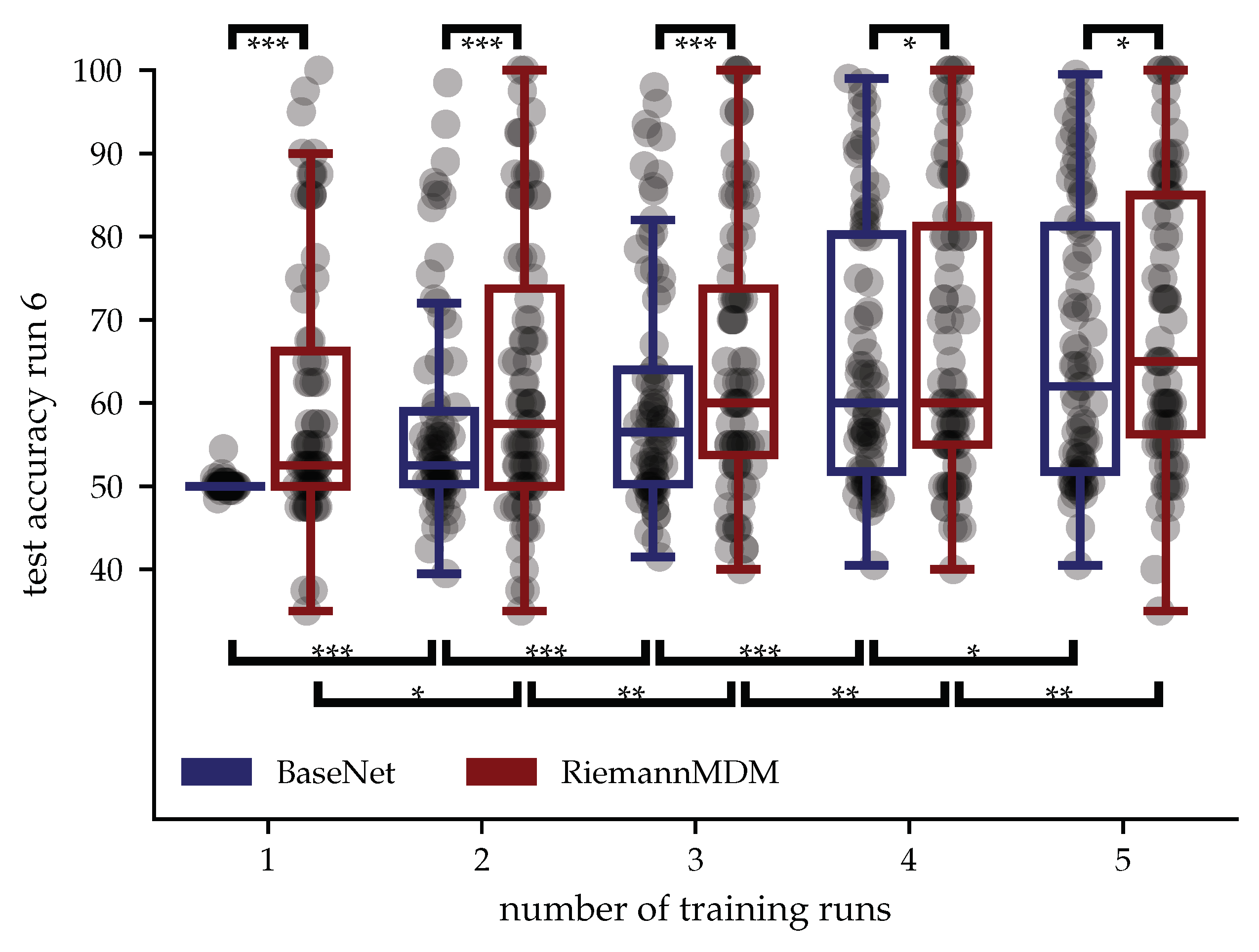
To investigate how the amount of training data influences the results for the within-subject setting, we trained the algorithms on the Dreyer2023 dataset and varied the amount of runs used for training. All runs were tested on the data from the last run. The results are displayed in Figure A1.
Figure A1.
Within-subject results for Dreyer2023 and different amounts of training data. Each dot resembles a subject, the stars within the brackets resemble the different significance levels (p<0.05(*), p<0.01(**) and p<0.001(***)) when comparing two experiments connected by that bracket.
Figure A1.
Within-subject results for Dreyer2023 and different amounts of training data. Each dot resembles a subject, the stars within the brackets resemble the different significance levels (p<0.05(*), p<0.01(**) and p<0.001(***)) when comparing two experiments connected by that bracket.
References
- Peksa, J. & Mamchur, D. State-of-the-Art on Brain-Computer Interface Technology. Sensors. 23, 6001 (2023). [CrossRef]
- Cervera, M., Soekadar, S., Ushiba, J., Millán, J., Liu, M., Birbaumer, N. & Garipelli, G. Brain-computer interfaces for post-stroke motor rehabilitation: a meta-analysis. Annals Of Clinical And Translational Neurology. 5, 651-663 (2018).
- Soekadar, S., Witkowski, M., Mellinger, J., Ramos, A., Birbaumer, N. & Cohen, L. ERD-based online brain-machine interfaces (BMI) in the context of neurorehabilitation: optimizing BMI learning and performance. IEEE Transactions On Neural Systems And Rehabilitation Engineering. 19, 542-549 (2011). [CrossRef]
- Decety, J. The neurophysiological basis of motor imagery. Behavioural Brain Research. 77, 45-52 (1996). [CrossRef]
- Lee, M., Kwon, O., Kim, Y., Kim, H., Lee, Y., Williamson, J., Fazli, S. & Lee, S. EEG dataset and OpenBMI toolbox for three BCI paradigms: An investigation into BCI illiteracy. GigaScience. 8, giz002 (2019). [CrossRef]
- Sannelli, C., Vidaurre, C., Müller, K. & Blankertz, B. A large scale screening study with a SMR-based BCI: Categorization of BCI users and differences in their SMR activity. PloS One. 14, e0207351 (2019). [CrossRef]
- Zhang, R., Li, F., Zhang, T., Yao, D. & Xu, P. Subject inefficiency phenomenon of motor imagery brain-computer interface: Influence factors and potential solutions. Brain Science Advances. 6, 224-241 (2020). [CrossRef]
- Perdikis, S., Tonin, L., Saeedi, S., Schneider, C. & Millán, J. The Cybathlon BCI race: Successful longitudinal mutual learning with two tetraplegic users. PLoS Biology. 16, e2003787 (2018). [CrossRef]
- Korik, A., McCreadie, K., McShane, N., Du Bois, N., Khodadadzadeh, M., Stow, J., McElligott, J., Carroll, Á. & Coyle, D. Competing at the Cybathlon championship for people with disabilities: long-term motor imagery brain–computer interface training of a cybathlete who has tetraplegia. Journal Of NeuroEngineering And Rehabilitation. 19, 95 (2022). [CrossRef]
- McFarland, D. & Wolpaw, J. Brain–computer interface use is a skill that user and system acquire together. PLoS Biology. 16, e2006719 (2018).
- Shenoy, K. & Carmena, J. Combining decoder design and neural adaptation in brain-machine interfaces. Neuron. 84, 665-680 (2014). [CrossRef]
- Orsborn, A., Moorman, H., Overduin, S., Shanechi, M., Dimitrov, D. & Carmena, J. Closed-loop decoder adaptation shapes neural plasticity for skillful neuroprosthetic control. Neuron. 82, 1380-1393 (2014). [CrossRef]
- Sitaram, R., Ros, T., Stoeckel, L., Haller, S., Scharnowski, F., Lewis-Peacock, J., Weiskopf, N., Blefari, M., Rana, M., Oblak, E. & Others Closed-loop brain training: the science of neurofeedback. Nature Reviews Neuroscience. 18, 86-100 (2017). [CrossRef]
- Kober, S., Witte, M., Ninaus, M., Neuper, C. & Wood, G. Learning to modulate one’s own brain activity: the effect of spontaneous mental strategies. Frontiers In Human Neuroscience. 7 pp. 695 (2013).
- Gaume, A., Vialatte, A., Mora-Sánchez, A., Ramdani, C. & Vialatte, F. A psychoengineering paradigm for the neurocognitive mechanisms of biofeedback and neurofeedback. Neuroscience & Biobehavioral Reviews. 68 pp. 891-910 (2016). [CrossRef]
- Mladenović, J., Mattout, J. & Lotte, F. A generic framework for adaptive EEG-based BCI training and operation. Brain–Computer Interfaces Handbook. pp. 595-612 (2018).
- Craik, A., He, Y. & Contreras-Vidal, J. Deep learning for electroencephalogram (EEG) classification tasks: a review. Journal Of Neural Engineering. 16, 031001 (2019). [CrossRef]
- Vavoulis, A., Figueiredo, P. & Vourvopoulos, A. A Review of Online Classification Performance in Motor Imagery-Based Brain-Computer Interfaces for Stroke Neurorehabilitation. Signals. 4, 73-86 (2023). [CrossRef]
- Tayeb, Z., Fedjaev, J., Ghaboosi, N., Richter, C., Everding, L., Qu, X., Wu, Y., Cheng, G. & Conradt, J. Validating deep neural networks for online decoding of motor imagery movements from EEG signals. Sensors. 19, 210 (2019). [CrossRef]
- Jeong, J., Shim, K., Kim, D. & Lee, S. Brain-controlled robotic arm system based on multi-directional CNN-BiLSTM network using EEG signals. IEEE Transactions On Neural Systems And Rehabilitation Engineering. 28, 1226-1238 (2020). [CrossRef]
- Karácsony, T., Hansen, J., Iversen, H. & Puthusserypady, S. Brain computer interface for neuro-rehabilitation with deep learning classification and virtual reality feedback. Proceedings Of The 10th Augmented Human International Conference 2019. pp. 1-8 (2019).
- Stieger, J., Engel, S., Suma, D. & He, B. Benefits of deep learning classification of continuous noninvasive brain–computer interface control. Journal Of Neural Engineering. 18, 046082 (2021). [CrossRef]
- Forenzo, D., Zhu, H., Shanahan, J., Lim, J. & He, B. Continuous tracking using deep learning-based decoding for noninvasive brain–computer interface. PNAS Nexus. 3, pgae145 (2024). [CrossRef]
- Schirrmeister, R., Springenberg, J., Fiederer, L., Glasstetter, M., Eggensperger, K., Tangermann, M., Hutter, F., Burgard, W. & Ball, T. Deep learning with convolutional neural networks for EEG decoding and visualization. Human Brain Mapping. 38, 5391-5420 (2017). [CrossRef]
- Lawhern, V., Solon, A., Waytowich, N., Gordon, S., Hung, C. & Lance, B. EEGNet: a compact convolutional neural network for EEG-based brain-computer interfaces. Journal Of Neural Engineering. 15, 056013 (2018). [CrossRef]
- Kumar, S., Alawieh, H., Racz, F., Fakhreddine, R. & Millán, J. Transfer learning promotes acquisition of individual BCI skills. PNAS Nexus. 3, pgae076 (2024). [CrossRef]
- Dreyer, P., Roc, A., Pillette, L., Rimbert, S. & Lotte, F. A large EEG database with users’ profile information for motor imagery brain-computer interface research. Scientific Data. 10, 580 (2023). [CrossRef]
- Sartzetaki, C., Antoniadis, P., Antonopoulos, N., Gkinis, I., Krasoulis, A., Perdikis, S. & Pitsikalis, V. Beyond Within-Subject Performance: A Multi-Dataset Study of Fine-Tuning in the EEG Domain. 2023 IEEE International Conference On Systems, Man, And Cybernetics (SMC). pp. 4429-4435 (2023).
- Wimpff, M., Gizzi, L., Zerfowski, J. & Yang, B. EEG motor imagery decoding: A framework for comparative analysis with channel attention mechanisms. Journal Of Neural Engineering. (2024). [CrossRef]
- Wimpff, M., Zerfowski, J. & Yang, B. Towards calibration-free online EEG motor imagery decoding using Deep Learning. ESANN 2024 Proceedings (2024), accepted.
- Wu, D., Jiang, X. & Peng, R. Transfer learning for motor imagery based brain–computer interfaces: A tutorial. Neural Networks. 153 pp. 235-253 (2022). [CrossRef]
- Ko, W., Jeon, E., Jeong, S., Phyo, J. & Suk, H. A survey on deep learning-based short/zero-calibration approaches for EEG-based brain–computer interfaces. Frontiers In Human Neuroscience. 15 pp. 643386 (2021). [CrossRef]
- Kostas, D. & Rudzicz, F. Thinker invariance: enabling deep neural networks for BCI across more people. Journal Of Neural Engineering. 17, 056008 (2020). [CrossRef]
- Sultana, M., Reichert, C., Sweeney-Reed, C. & Perdikis, S. Towards Calibration-Less BCI-Based Rehabilitation. 2023 IEEE International Conference On Metrology For EXtended Reality, Artificial Intelligence And Neural Engineering (MetroXRAINE). pp. 11-16 (2023).
- Han, J., Wei, X. & Faisal, A. EEG decoding for datasets with heterogenous electrode configurations using transfer learning graph neural networks. Journal Of Neural Engineering. 20, 066027 (2023). [CrossRef]
- Jiménez-Guarneros, M. & Gómez-Gil, P. Custom Domain Adaptation: A new method for cross-subject, EEG-based cognitive load recognition. IEEE Signal Processing Letters. 27 pp. 750-754 (2020). [CrossRef]
- He, H. & Wu, D. Different set domain adaptation for brain-computer interfaces: A label alignment approach. IEEE Transactions On Neural Systems And Rehabilitation Engineering. 28, 1091-1108 (2020). [CrossRef]
- Han, J., Wei, X. & Faisal, A. EEG decoding for datasets with heterogenous electrode configurations using transfer learning graph neural networks. Journal Of Neural Engineering. 20, 066027 (2023). [CrossRef]
- Gu, X., Han, J., Yang, G. & Lo, B. Generalizable Movement Intention Recognition with Multiple Heterogeneous EEG Datasets. 2023 IEEE International Conference On Robotics And Automation (ICRA). pp. 9858-9864 (2023).
- Ju, C., Gao, D., Mane, R., Tan, B., Liu, Y. & Guan, C. Federated transfer learning for EEG signal classification. 2020 42nd Annual International Conference Of The IEEE Engineering In Medicine & Biology Society (EMBC). pp. 3040-3045 (2020).
- Mao, T., Li, C., Zhao, Y., Song, R. & Chen, X. Online test-time adaptation for patient-independent seizure prediction. IEEE Sensors Journal. (2023). [CrossRef]
- Wang, K., Yang, M., Li, C., Liu, A., Qian, R. & Chen, X. Privacy-Preserving Domain Adaptation for Intracranial EEG Classification via Information Maximization and Gaussian Mixture Model. IEEE Sensors Journal. (2023). [CrossRef]
- Xia, K., Deng, L., Duch, W. & Wu, D. Privacy-preserving domain adaptation for motor imagery-based brain-computer interfaces. IEEE Transactions On Biomedical Engineering. 69, 3365-3376 (2022). [CrossRef]
- Li, S., Wang, Z., Luo, H., Ding, L. & Wu, D. T-TIME: Test-time information maximization ensemble for plug-and-play BCIs. IEEE Transactions On Biomedical Engineering. (2023). [CrossRef]
- Wimpff, M., Döbler, M. & Yang, B. Calibration-free online test-time adaptation for electroencephalography motor imagery decoding. 2024 12th International Winter Conference On Brain-Computer Interface (BCI). pp. 1-6 (2024).
- Guetschel, P. & Tangermann, M. Transfer Learning between Motor Imagery Datasets using Deep Learning–Validation of Framework and Comparison of Datasets. ArXiv Preprint ArXiv:2311.16109. (2023).
- Ouahidi, Y., Gripon, V., Pasdeloup, B., Bouallegue, G., Farrugia, N. & Lioi, G. A Strong and Simple Deep Learning Baseline for BCI MI Decoding. ArXiv Preprint ArXiv:2309.07159. (2023).
- Xie, Y., Wang, K., Meng, J., Yue, J., Meng, L., Yi, W., Jung, T., Xu, M. & Ming, D. Cross-dataset transfer learning for motor imagery signal classification via multi-task learning and pre-training. Journal Of Neural Engineering. 20, 056037 (2023). [CrossRef]
- Xu, Y., Huang, X. & Lan, Q. Selective cross-subject transfer learning based on riemannian tangent space for motor imagery brain-computer interface. Frontiers In Neuroscience. 15 pp. 779231 (2021). [CrossRef]
- An, S., Kim, S., Chikontwe, P. & Park, S. Few-shot relation learning with attention for EEG-based motor imagery classification. 2020 IEEE/RSJ International Conference On Intelligent Robots And Systems (IROS). pp. 10933-10938 (2020).
- Junqueira, B., Aristimunha, B., Chevallier, S. & Camargo, R. A systematic evaluation of Euclidean alignment with deep learning for EEG decoding. Journal Of Neural Engineering. (2024). [CrossRef]
- Liu, S., Zhang, J., Wang, A., Wu, H., Zhao, Q. & Long, J. Subject adaptation convolutional neural network for EEG-based motor imagery classification. Journal Of Neural Engineering. 19, 066003 (2022). [CrossRef]
- Duan, T., Chauhan, M., Shaikh, M., Chu, J. & Srihari, S. Ultra Efficient Transfer Learning with Meta Update for Continuous EEG Classification Across Subjects.. Canadian Conference On AI. (2021). [CrossRef]
- Ouahidi, Y., Lioi, G., Farrugia, N., Pasdeloup, B. & Gripon, V. Unsupervised Adaptive Deep Learning Method For BCI Motor Imagery Decoding. ArXiv Preprint ArXiv:2403.15438. (2024).
- Xu, L., Ma, Z., Meng, J., Xu, M., Jung, T. & Ming, D. Improving transfer performance of deep learning with adaptive batch normalization for brain-computer interfaces. 2021 43rd Annual International Conference Of The IEEE Engineering In Medicine & Biology Society (EMBC). pp. 5800-5803 (2021).
- Gu, X., Han, J., Yang, G. & Lo, B. Generalizable Movement Intention Recognition with Multiple Heterogeneous EEG Datasets. 2023 IEEE International Conference On Robotics And Automation (ICRA). pp. 9858-9864 (2023).
- Bakas, S., Ludwig, S., Adamos, D., Laskaris, N., Panagakis, Y. & Zafeiriou, S. Latent Alignment with Deep Set EEG Decoders. ArXiv Preprint ArXiv:2311.17968. (2023).
- Zhuo, F., Zhang, X., Tang, F., Yu, Y. & Liu, L. Riemannian transfer learning based on log-Euclidean metric for EEG classification. Frontiers In Neuroscience. 18 pp. 1381572 (2024). [CrossRef]
- Zhang, W. & Wu, D. Manifold embedded knowledge transfer for brain-computer interfaces. IEEE Transactions On Neural Systems And Rehabilitation Engineering. 28, 1117-1127 (2020).
- He, H. & Wu, D. Transfer learning for brain–computer interfaces: A Euclidean space data alignment approach. IEEE Transactions On Biomedical Engineering. 67, 399-410 (2019).
- Xu, L., Xu, M., Ke, Y., An, X., Liu, S. & Ming, D. Cross-dataset variability problem in EEG decoding with deep learning. Frontiers In Human Neuroscience. 14 pp. 103 (2020). [CrossRef]
- Zoumpourlis, G. & Patras, I. Motor imagery decoding using ensemble curriculum learning and collaborative training. 2024 12th International Winter Conference On Brain-Computer Interface (BCI). pp. 1-8 (2024).
- Zanini, P., Congedo, M., Jutten, C., Said, S. & Berthoumieu, Y. Transfer learning: A Riemannian geometry framework with applications to brain–computer interfaces. IEEE Transactions On Biomedical Engineering. 65, 1107-1116 (2017). [CrossRef]
- Li, Y., Wang, N., Shi, J., Liu, J. & Hou, X. Revisiting batch normalization for practical domain adaptation. ArXiv Preprint ArXiv:1603.04779. (2016).
- Schneider, S., Rusak, E., Eck, L., Bringmann, O., Brendel, W. & Bethge, M. Improving robustness against common corruptions by covariate shift adaptation. Advances In Neural Information Processing Systems. 33 pp. 11539-11551 (2020).
- Döbler, M., Marsden, R. & Yang, B. Robust mean teacher for continual and gradual test-time adaptation. Proceedings Of The IEEE/CVF Conference On Computer Vision And Pattern Recognition. pp. 7704-7714 (2023).
- Marsden, R., Döbler, M. & Yang, B. Universal test-time adaptation through weight ensembling, diversity weighting, and prior correction. Proceedings Of The IEEE/CVF Winter Conference On Applications Of Computer Vision. pp. 2555-2565 (2024).
Figure 1.
Trial structure for both datasets. Each trial starts with a fixation cross. For the Dreyer2023 dataset this is followed by an auditory signal. The cue occurs after 3 seconds for both datasets. For the Dreyer2023 dataset the cue is present for 1.25 seconds and followed by a 3.75 second feedback phase. For the Lee2029 dataset, the cue is present during the whole trial and the feedback is indicated by the position of a small cross within the cue arrow. Between the trials a blank screen is displayed. The time period used for classification is indicated by the green outline.
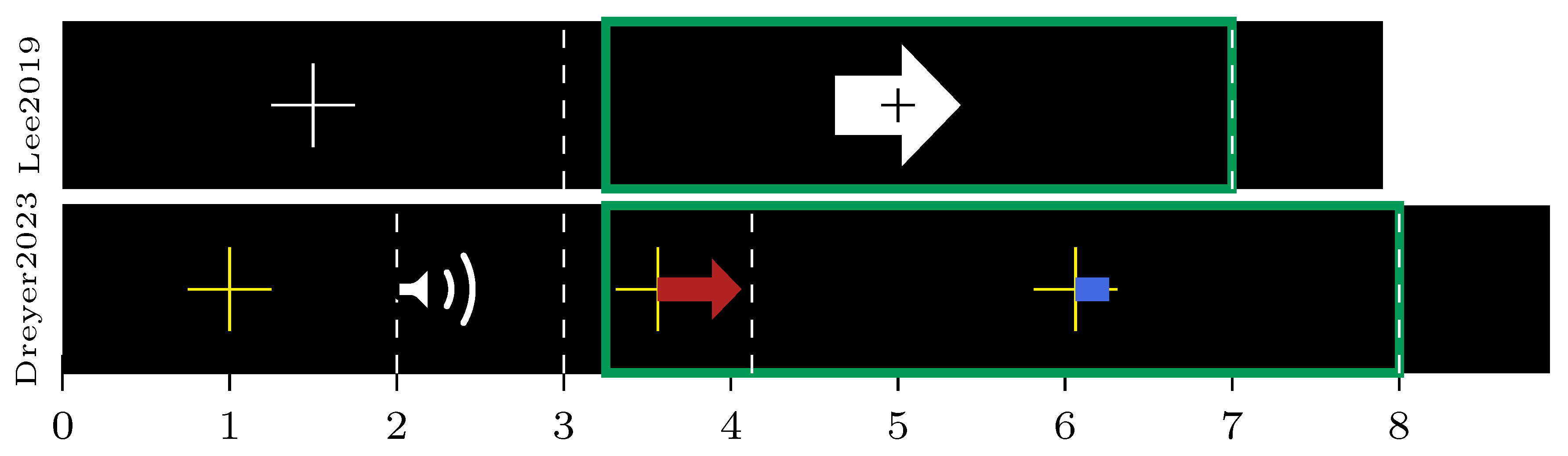
Figure 2.
A) BaseNet architecture and output dimensions of joint decoding (upper illustration) and individual windows (lower illustration) for the Dreyer2023 dataset. Layer names are specified following the PyTorch API conventions. For Conv2d layers, the first value indicates the number of filters, and the tuple represents the kernel size. In the pooling layers, the first tuple indicates the kernel size, while the second tuple specifies the stride. B) Visualization of the sliding window extraction in the second pooling layer of BaseNet.
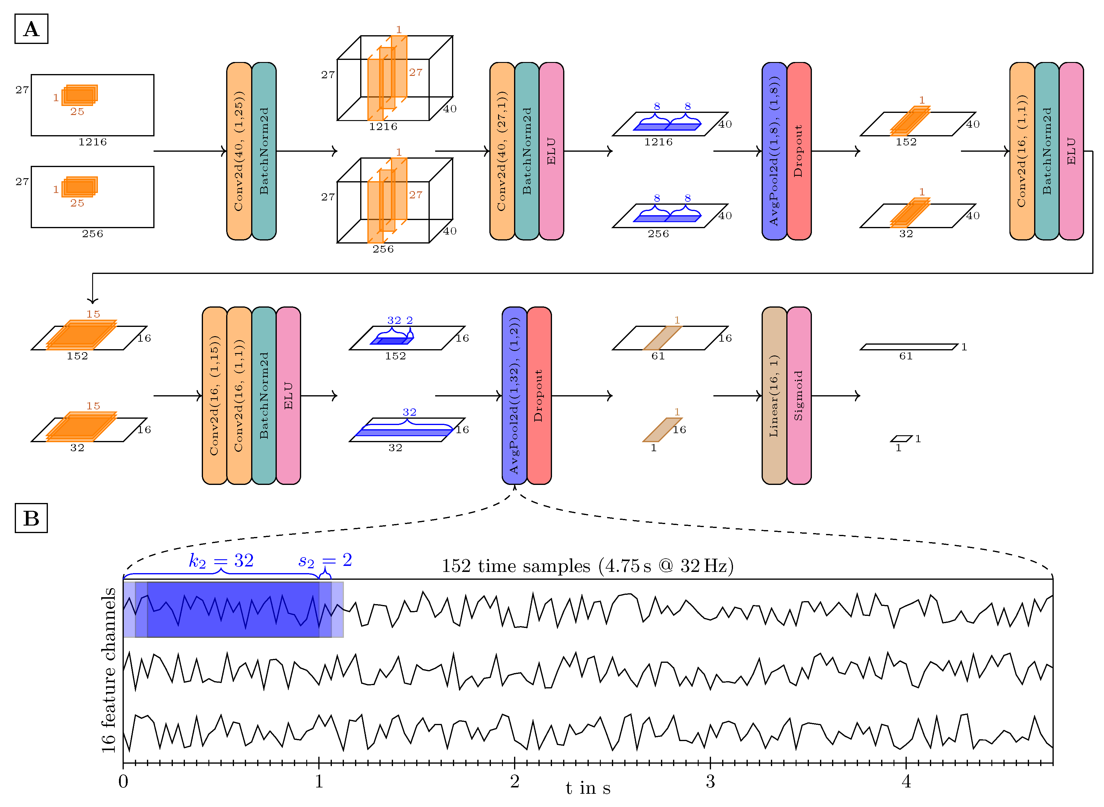
Figure 3.
Computational gain of joint decoding for and different trial lengths and window lengths .
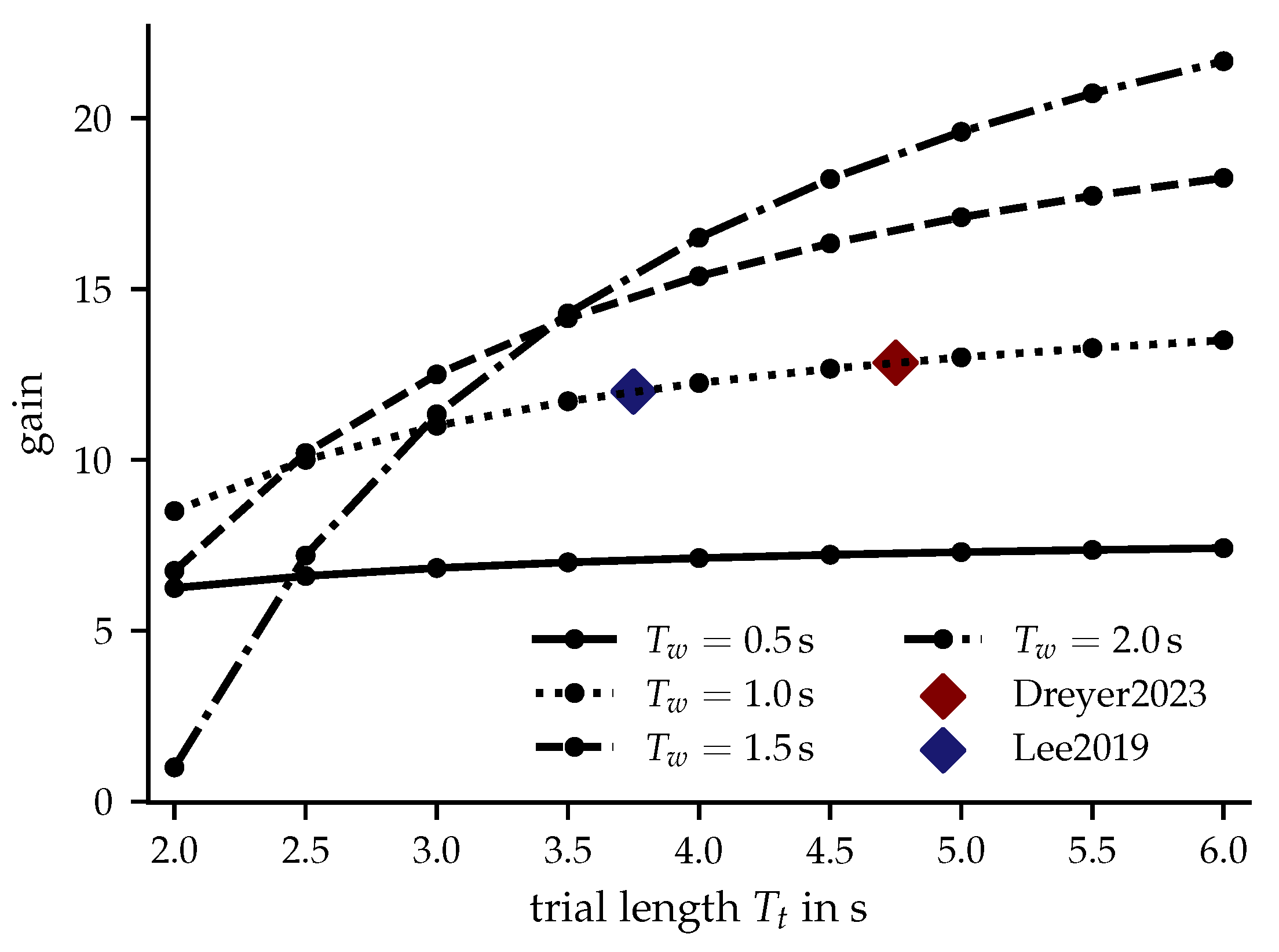
Figure 4.
Simplified overview of the domain adaptation landscape. Italic text specifies requirements regarding calibration data.
Figure 4.
Simplified overview of the domain adaptation landscape. Italic text specifies requirements regarding calibration data.
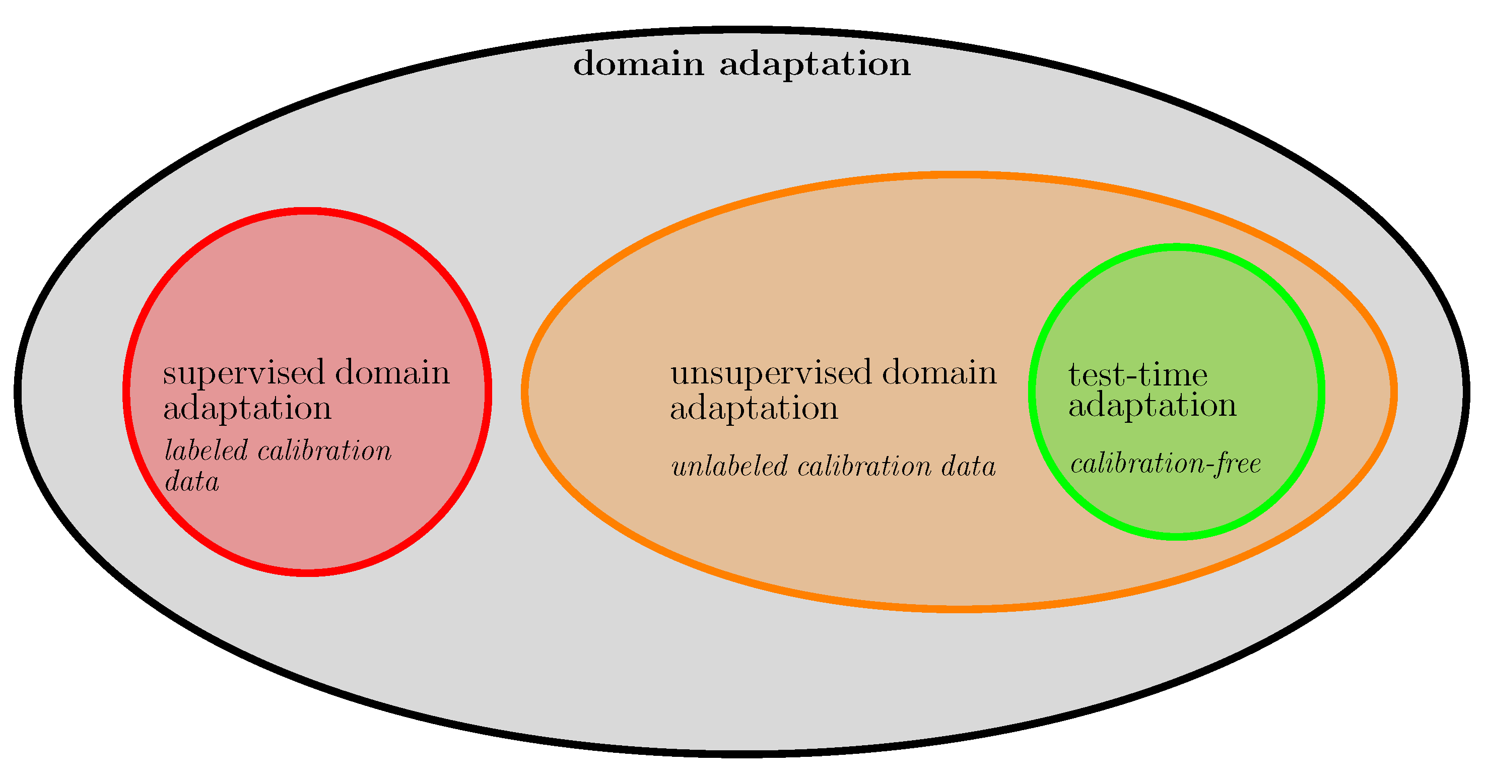
Figure 5.
Cross-subject results for the Dreyer2023 dataset for different data compositions. Each dot resembles a subject, the stars within the brackets resemble the different significance levels (p<0.05(*), p<0.01(**) and p<0.001(***)) when comparing two experiments connected by that bracket.
Figure 5.
Cross-subject results for the Dreyer2023 dataset for different data compositions. Each dot resembles a subject, the stars within the brackets resemble the different significance levels (p<0.05(*), p<0.01(**) and p<0.001(***)) when comparing two experiments connected by that bracket.
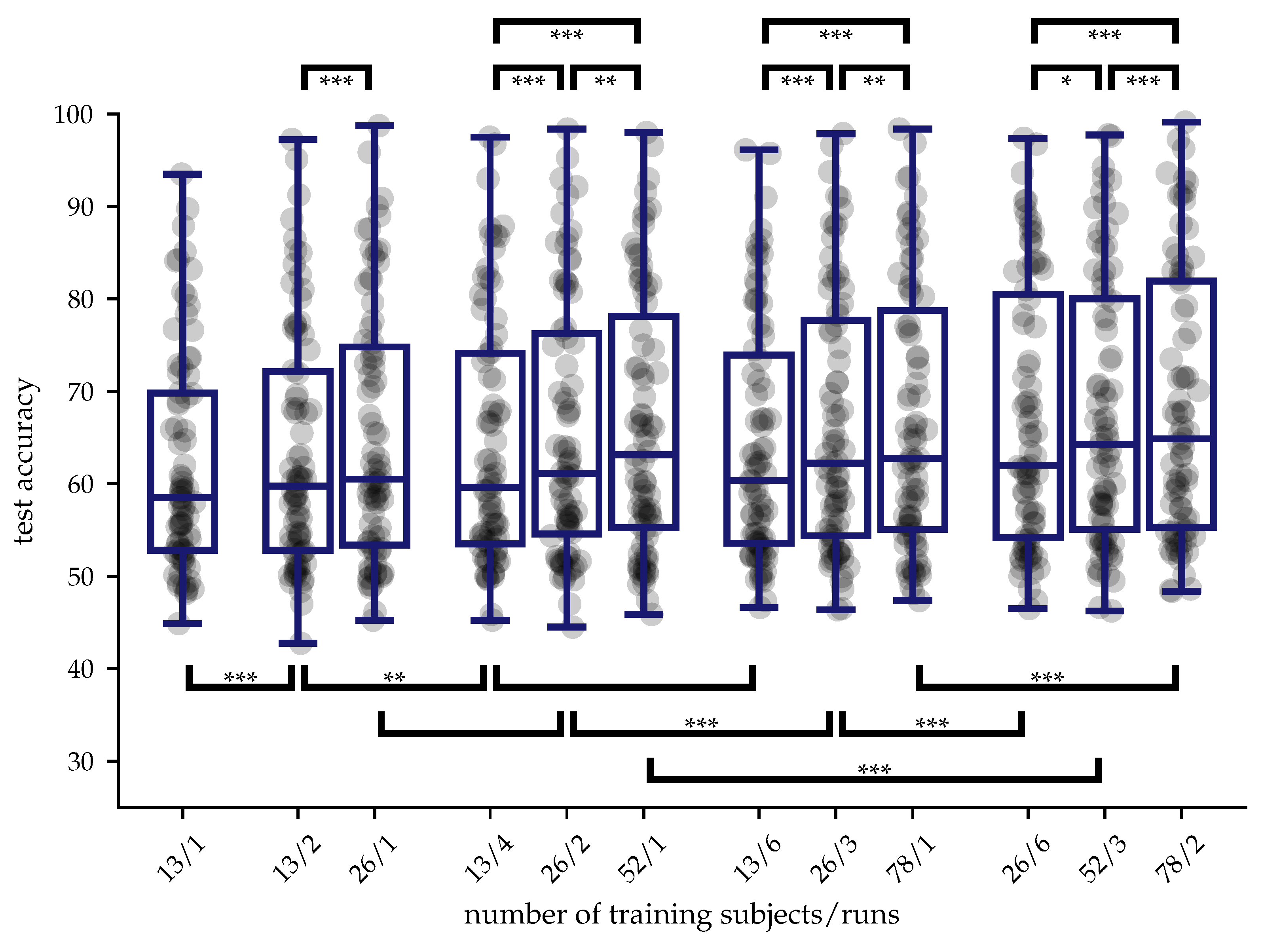
Figure 6.
Cross-subject results for the Lee2019 dataset for different data compositions. Each dot resembles a subject, the stars within the brackets resemble the different significance levels (p<0.05(*), p<0.01(**) and p<0.001(***)) when comparing two experiments connected by that bracket.
Figure 6.
Cross-subject results for the Lee2019 dataset for different data compositions. Each dot resembles a subject, the stars within the brackets resemble the different significance levels (p<0.05(*), p<0.01(**) and p<0.001(***)) when comparing two experiments connected by that bracket.
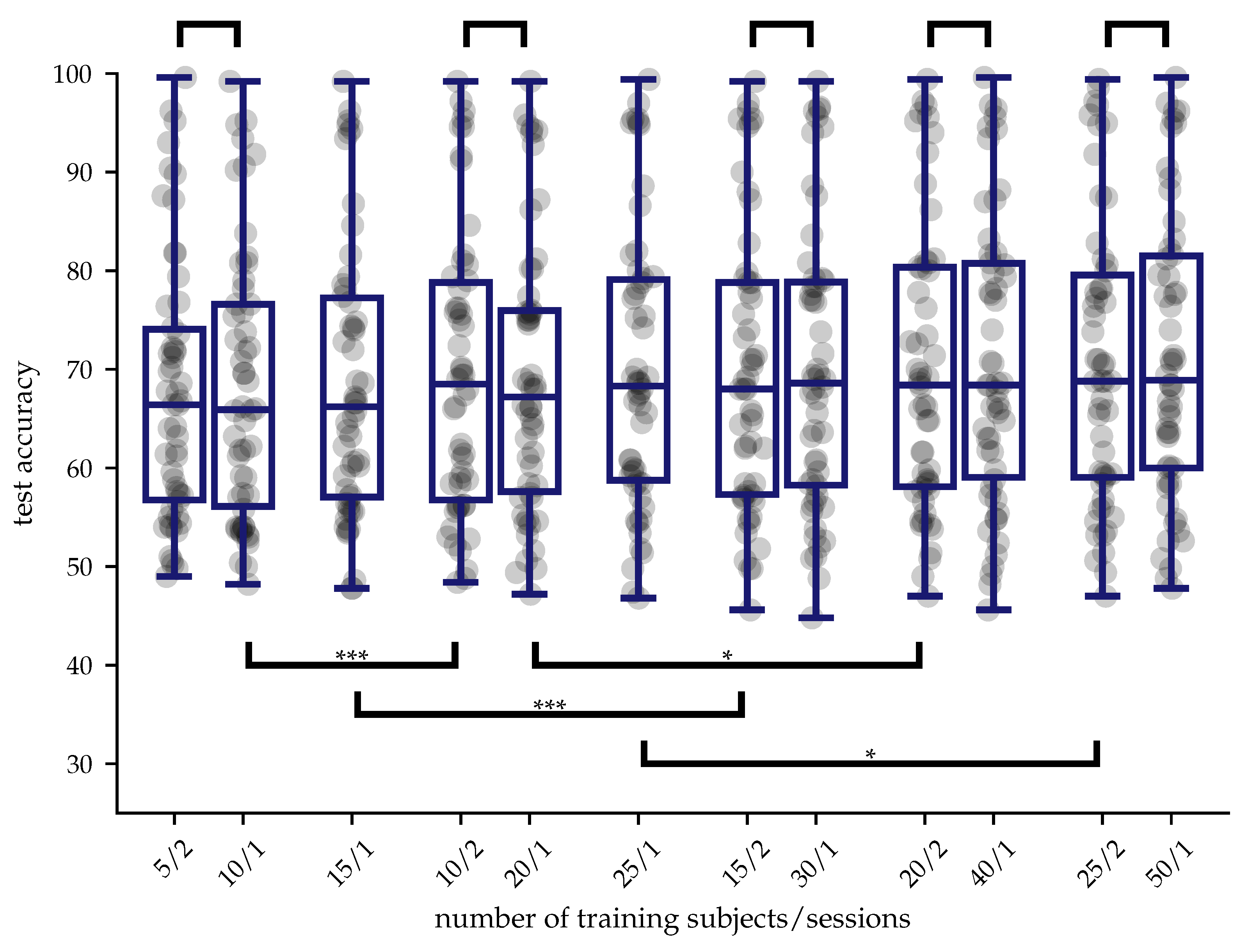
Figure 7.
Accuracy and samples per entropy bin for BaseNet (width of each bin equals 0.1, starting from 0). Each black dot resembles one subject. The trials are averaged over the seeds but the accuracies are filtered, i.e., accuracies where no trials were in the entropy bin are removed and thus no averaging can be performed.
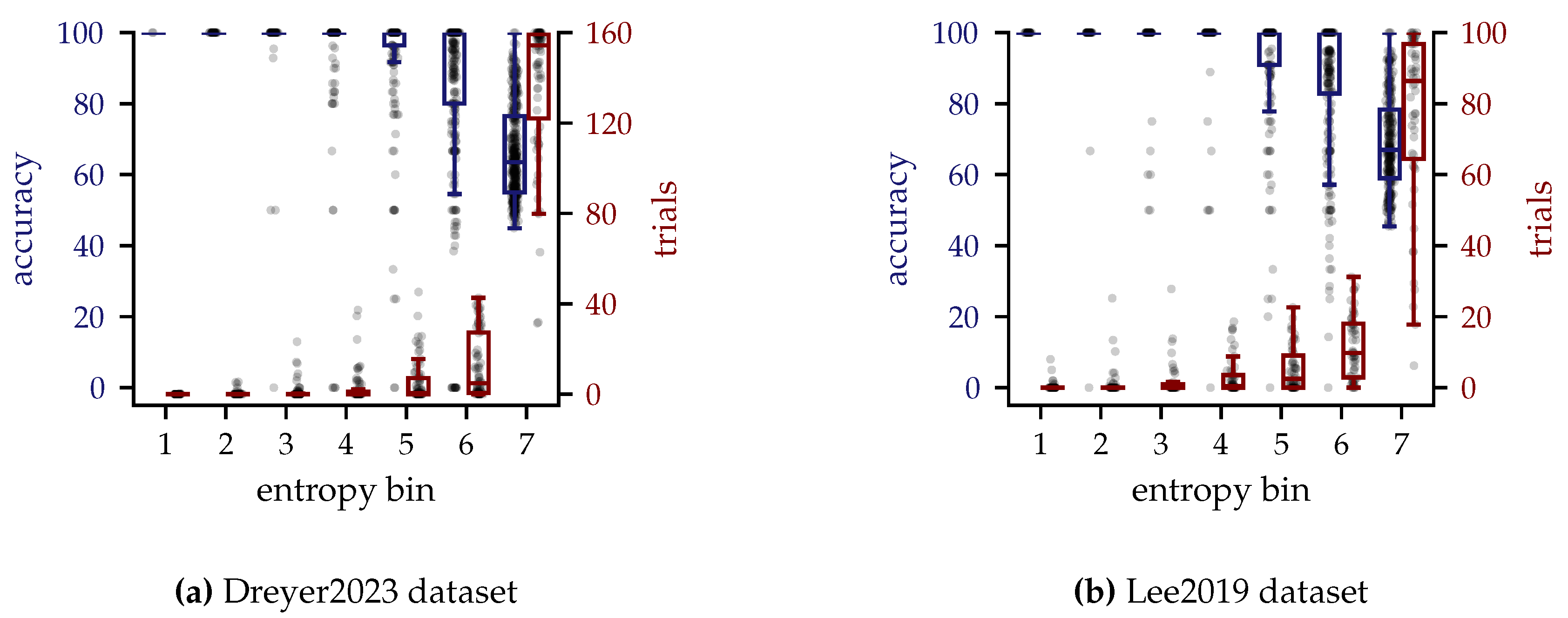
Figure 8.
Accuracies per window for BaseNet. Each black line indicates one subject, the red line corresponds to the average and the blue lines correspond to the average ± standard deviation.
Figure 8.
Accuracies per window for BaseNet. Each black line indicates one subject, the red line corresponds to the average and the blue lines correspond to the average ± standard deviation.
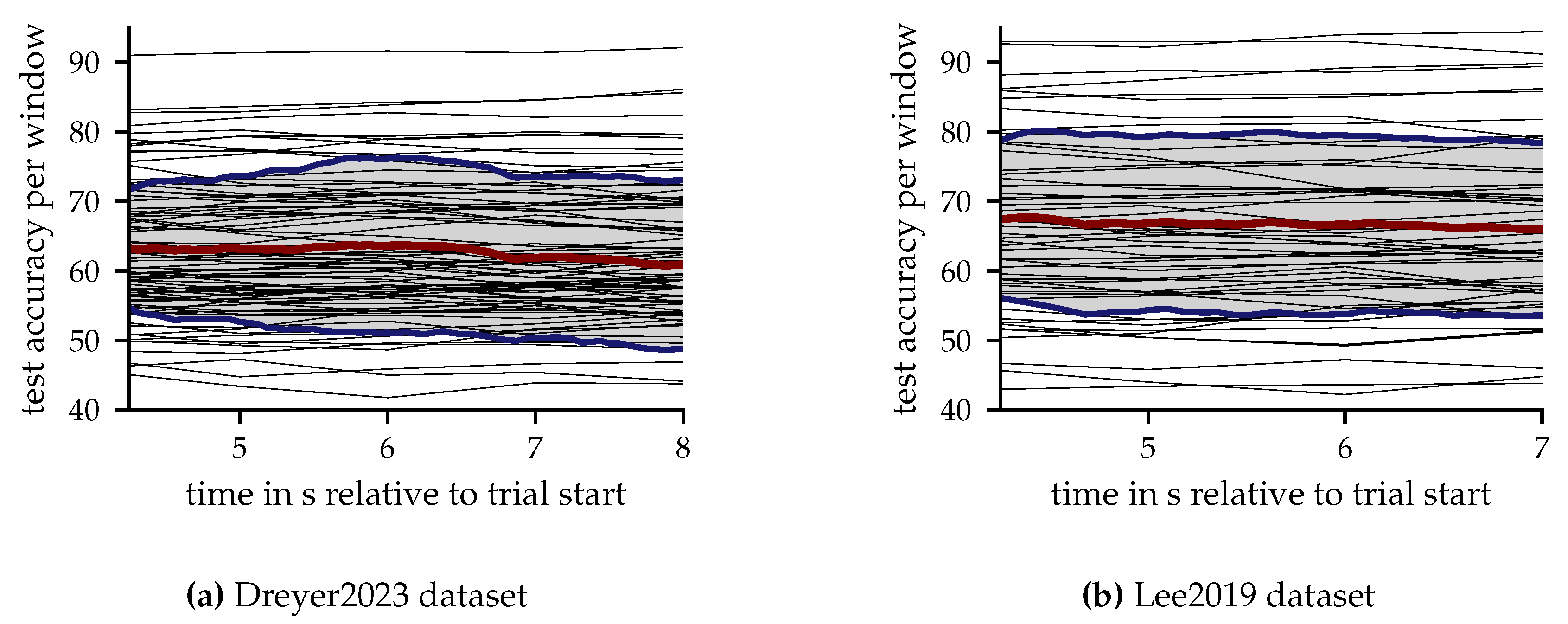
Figure 9.
Topoplots of the EDS scores for BaseNet and both datasets. Good subjects have a TAcc > 70%, bad subjects yield a performance below or equal to this threshold.
Figure 9.
Topoplots of the EDS scores for BaseNet and both datasets. Good subjects have a TAcc > 70%, bad subjects yield a performance below or equal to this threshold.
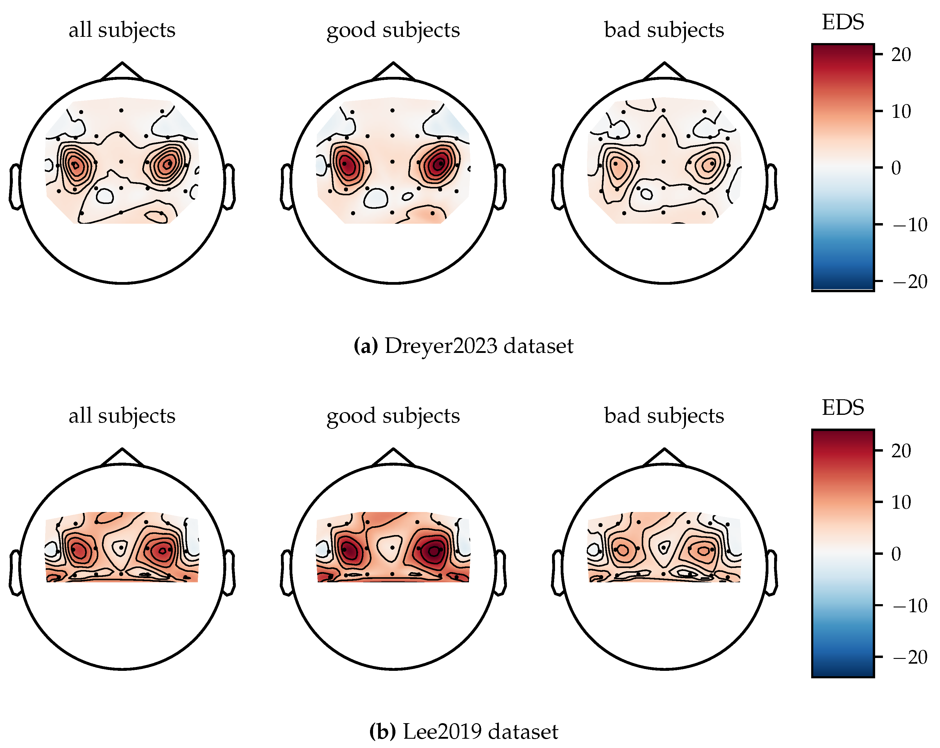
Table 1.
Within-subject results. Results above the double line are for the Dreyer2023 dataset, below are for the Lee2019 dataset.
Table 1.
Within-subject results. Results above the double line are for the Dreyer2023 dataset, below are for the Lee2019 dataset.
| Method | TAcc(%) | uTacc(%) | WAcc(%) |
|---|---|---|---|
| RiemannMDM (p<0.001) | |||
| BaseNet | |||
| RiemannMDM (p=0.065) | |||
| BaseNet |
Table 2.
Dreyer2023 dataset cross-subject experiments. The stars after the method indicate the different significance levels (p<0.05(*), p<0.01(**) and p<0.001(***)) compared to the benchmark method in the same setting.
Table 2.
Dreyer2023 dataset cross-subject experiments. The stars after the method indicate the different significance levels (p<0.05(*), p<0.01(**) and p<0.001(***)) compared to the benchmark method in the same setting.
| Method | TAcc(%) | uTacc(%) | WAcc(%) | |
| BaseNet | ||||
| supervised | RiemannMDM+PAR | |||
| BaseNet*** | ||||
| BaseNet+EA*** | ||||
| BaseNet+RA*** | ||||
| unsupervised | RiemannMDM | |||
| BaseNet+EA*** | ||||
| BaseNet+RA*** | ||||
| BaseNet+AdaBN** | ||||
| BaseNet+EA+AdaBN*** | ||||
| BaseNet+RA+AdaBN*** | ||||
| online | RiemannMDM+GR | |||
| BaseNet+EA* | ||||
| BaseNet+RA** | ||||
| BaseNet+AdaBN (p=0.125) | ||||
| BaseNet+EA+AdaBN** | ||||
| BaseNet+RA+AdaBN** |
Table 3.
Lee2019 cross-subject experiments. The stars after the method indicate the different significance levels (p<0.05(*), p<0.01(**) and p<0.001(***)) compared to the benchmark method in the same setting.
Table 3.
Lee2019 cross-subject experiments. The stars after the method indicate the different significance levels (p<0.05(*), p<0.01(**) and p<0.001(***)) compared to the benchmark method in the same setting.
| Method | TAcc(%) | uTacc(%) | WAcc(%) | |
| BaseNet | ||||
| supervised | RiemannMDM+PAR | |||
| BaseNet*** | ||||
| BaseNet+EA*** | ||||
| BaseNet+RA*** | ||||
| unsupervised | RiemannMDM | |||
| BaseNet+EA*** | ||||
| BaseNet+RA*** | ||||
| BaseNet+AdaBN*** | ||||
| BaseNet+EA+AdaBN*** | ||||
| BaseNet+RA+AdaBN*** | ||||
| online | RiemannMDM+GR | |||
| BaseNet+EA*** | ||||
| BaseNet+RA*** | ||||
| BaseNet+AdaBN* | ||||
| BaseNet+EA+AdaBN*** | ||||
| BaseNet+RA+AdaBN*** |
Disclaimer/Publisher’s Note: The statements, opinions and data contained in all publications are solely those of the individual author(s) and contributor(s) and not of MDPI and/or the editor(s). MDPI and/or the editor(s) disclaim responsibility for any injury to people or property resulting from any ideas, methods, instructions or products referred to in the content. |
© 2024 by the authors. Licensee MDPI, Basel, Switzerland. This article is an open access article distributed under the terms and conditions of the Creative Commons Attribution (CC BY) license (http://creativecommons.org/licenses/by/4.0/).
Copyright: This open access article is published under a Creative Commons CC BY 4.0 license, which permit the free download, distribution, and reuse, provided that the author and preprint are cited in any reuse.


