A Petri Net-based Algorithm for Solving the One-Dimensional Cutting Stock Problem

Preprint

Article

A Petri Net-based Algorithm for Solving the One-Dimensional Cutting Stock Problem

Altmetrics

Downloads

Views

Comments

A peer-reviewed article of this preprint also exists.

Irving Barragan-Vite^*

Joselito Medina-Marin

Norberto Hernandez-Romero

Gustavo Erick Anaya-Fuentes

Irving Barragan-Vite^*

Joselito Medina-Marin

Norberto Hernandez-Romero

Gustavo Erick Anaya-Fuentes

This version is not peer-reviewed

Submitted:

29 July 2024

Posted:

30 July 2024

You are already at the latest version

Alerts

Abstract

Cutting and packing problems have been studied for decades and are of concern for a wide variety of industries to reduce costs and material utilization. This paper addresses the one-dimensional cutting stock problem, focusing on minimizing total stock usage. Procedures that address this problem include linear programming methods and metaheuristics. However, linear programming methods are limited to low-complexity instances, while most metaheuristics require extensive parameter tuning. In this paper, we develop a Petri-net model to construct cutting patterns. Using the reachability tree of the Petri net, the filtered beam search algorithm is implemented to find the best solution. Our algorithm is compared with the Least Lost Algorithm and the Generate & Solve algorithm over five datasets of instances. These algorithms share some characteristics with ours and have proven to be effective and efficient. Experimental results demonstrate that our algorithm effectively finds optimal solutions for both low and high-complexity instances. These findings confirm that Petri nets are suitable for modeling and solving the one-dimensional cutting stock problem.

Keywords:

Subject: Engineering - Industrial and Manufacturing Engineering

1. Introduction

Cutting stock problems are combinatorial problems involving the creation of small objects from large objects according to a cutting plan made of cutting patterns. The larger the number of small objects, the greater the number of possible cutting patterns, and hence these problems are classified as NP-hard optimization problems [1]. In this study, we focus on the single stock-size cutting problem according to Wascher’s classification [2] for the one-dimensional case, or one-dimensional cutting stock problem (1D-CSP), as it is best known in most of the literature. The 1D-CSP arises in industries manufacturing goods from paper, metal, glass, and wood, among others. The goal is the reduction of material usage and, therefore, the minimization of the related costs. Apart from cost reduction, industries such as the building industry are concerned with reducing gas emissions due to metal and concrete usage, as pointed out in [3]. Some other studies also address the problem by considering mathematical models that include the reuse of leftovers, as in [4].

Most approaches to solving the 1D-CSP are based on linear programming (LP) methods, with the column generation technique being one of the most outstanding ones. Reference [5] presents some LP formulations proposed in the early stages of addressing the 1D-CSP. Additionally, a comprehensive survey of LP methods used to solve the 1D-CSP up to 2015 can be found in [6]. Column generation and other techniques focus on generating and reducing the number of cutting patterns. In the 1D-CSP, a cutting pattern is an ordered sequence of items cut from a large object or stock. One-cut models and arc-flow models are other paradigms used to address the 1D-CSP, as solutions to the 1D-CSP can be constructed as sequences of items. It is well-known that LP methods can yield optimal solutions to the 1D-CSP, provided that the complexity of the instances is small, that is, with a small number of small objects or items. This limitation has led to the use of heuristic and metaheuristic approaches. Although these methods usually result in near-optimal solutions, the computational time is typically higher compared to LP methods. Additionally, a drawback of using metaheuristics is the complexity of solution representation and the numerous parameters that must be set and tuned. Since a solution for the 1D-CSP can be sequentially constructed, we propose using ordinary Petri nets (PN) to model the solution construction. We take advantage of the reachability tree to find the best solution through the implementation of a filtered beam search algorithm (FBS). Beam search algorithms are a type of any-time search algorithm, suitable for optimization problems where solutions can be constructed sequentially and represented as a tree structure. Unlike other any-time search methods, beam search algorithms do not perform backtracking. Only the most promising nodes at each level are retained to continue searching for the best path from the root node to a desired final node, while non-promising nodes are pruned permanently. The FBS is an improvement to the classical beam search algorithm. At each level, it first filters the nodes through a local evaluation and then performs a global evaluation among the filtered nodes to retain the best ones for further investigation.

In the literature, most mathematical models for the 1D-CSP consider single-objective functions. However, [7] demonstrated the effectiveness of using a bi-objective function. In this study, we consider the bi-objective function of the mathematical model (1)-(3) based on the one used in [8] for the 1D-CSP without contiguity. The objective function to be minimized accounts for both the minimization of waste and the minimization of the number of stocks with waste.

\begin{matrix} \min & W = \frac{1}{k + 1} (\sum_{j = 1}^{k} \sqrt{\frac{w_{j}}{L_{j}}} + \sum_{j = 1}^{k} \frac{V_{j}}{k}) \end{matrix}

(1)

\begin{matrix} subject to \\ \sum_{j = 1}^{k} x_{i j} = d_{i}, i = 1, 2, \dots, m \end{matrix}

(2)

\begin{matrix} x_{i j} \geq 0 and integer . \end{matrix}

(3)

In model (1)-(3),

L_{j}

is the length of the stock, m is the number of different items, k is the total number of stocks used.

d_{i}

represents the demand or total number of orders of item i, while

l_{i}

is the length of item i,

x_{i j}

is the number of orders of item i in stock j.

w_{j}

and

V_{j}

are defined in Equations (4) and (5), respectively, where

w_{j}

represents the wastage of stock j.

\begin{matrix} w_{j} & = L_{j} - \sum_{i = 1}^{m} x_{i j} l_{i}, j = 1, 2, \dots, k \end{matrix}

(4)

\begin{matrix} V_{j} & = \{\begin{matrix} 1 & if & w_{j} > 0, & j = 1, 2, \dots, k \\ 0 & otherwise . \end{matrix} \end{matrix}

(5)

Even though the main drawback of PN is state explosion, we do not generate the complete reachability tree. Instead, we generate promising states from the initial state that lead to the desired final state with minimum waste, according to the FBS, using the bi-objective function (1) to evaluate the nodes. The initial state or marking of the PN is where no items have been taken to form a solution, and the final state or marking is where all items have been taken to form a solution. At each level of the tree, partial solutions are evaluated locally, and the best ones are then evaluated globally. Nodes with the best partial solutions are kept for further investigation. The advantages of using PN are twofold: they are useful for validating solutions when PN is deadlock-free, and they can be combined with graph search methods to solve optimization problems. Some of the problems addressed under the PN paradigm include job and flow shop scheduling problems. In these cases, PN and graph search methods like

A^{*}

algorithms [9,10,11,12] and beam search algorithms [13,14,15,16] have been used to obtain the best scheduling solutions. However, to the best of our knowledge, PN has not been used to solve cutting problems. Our experimental results show that PN is suitable for modeling pattern generation and solving the 1D-CSP, with acceptable performance in both solution quality and computational time.

2. Literature Review

It is widely considered that Kantorovich first addressed the 1D-CSP in [17] providing an LP formulation of the problem and using the multipliers method to solve it. Later, [18,19] used the column generation technique to solve the integer linear programming formulation by addressing an associated knapsack problem. Following the introduction of the column generation technique, several procedures were developed to improve its computational performance using branch-and-price algorithms [20,21,22,23]. Other algorithms have focused on constructing and reducing the number of patterns [24,25,26,27,28]. Alternative approaches to modeling and solving the 1D-CSP include the arc-flow and one-cut formulations. The arc-flow formulation, a graph-based approach, was introduced in [29]. Recently [30] proposed and compared arc-flow formulations based on other algorithms. One-cut formulations have received little attention since their use in [31]. Moreover, [32] proved the equivalence among pattern-based formulations, such as that of Gilmore & Gomory [18,19], and the arc-flow and one-cut formulations. [33] used dynamic programming to solve the 1D-CSP, and [34] showed the relationship between arc-flow formulations and dynamic programming in solving optimization problems.

LP methods are restricted to instances of a small number of items, and to overcome this limitation, many researchers have proposed metaheuristic methods like genetic algorithms [35,36,37]. However, the use of genetic algorithms faces the difficulty of finding the best way to encode the solutions or cutting patterns, as pointed out in [38,39,40,41]. Evolutionary programming was used in [8,42] to address the 1D-CSP with and without contiguity. Additionally, [43] concluded that evolutionary programming performs better than genetic algorithms for solving the 1D-CSP. Swarm intelligence algorithms, such as particle swarm optimization algorithms [44,45,46,47] and ant colony optimization algorithms [48,49,50], have also been used to solve the 1D-CSP. The main issues with these two algorithms are parameter tuning and the need for hybridizations to avoid premature convergence and control the search space. Additionally, discretization procedures are required since these algorithms are better suited for continuous problems. Other metaheuristic algorithms for solving the 1D-CSP include tabu search, simulated annealing [51], and iterative local search [52,53]. More recently, [54] introduced the least-lost algorithm to simultaneously minimize waste and stocks with waste in the 1D-CSP, showing better results than the evolutionary programming algorithm of [8]. [55] compares a Generate & Solve algorithm to the column generation technique. The Generate & Solve algorithm uses a reduction technique based on the one presented in [56] to deal with large instances of the 1D-CSP. Although the algorithm is not better than the column generation technique, it can solve larger instances in acceptable computational time with quasi-optimal solutions. [57] introduces a deep reinforcement learning algorithm to minimize the number of stocks and maximize the length of leftovers. The algorithm performs well in terms of computational time and handling large instances.

3. Basic Concepts

In this section, we present the basic concepts of ordinary PN and the beam search algorithm necessary for introducing our algorithm. However, PN theory is extensive, so readers are referred to [58] for more information on the properties and variants of PN.

3.1. Petri Nets

PN were introduced by Carl A. Petri in 1960 as part of his doctoral dissertation. Since then, many researchers have studied PN theory and its applications. Additionally, other types of PN, such as timed PN, colored PN, and stochastic PN, have been developed to enhance their modeling power. In this paper, we will refer to the ordinary PN.

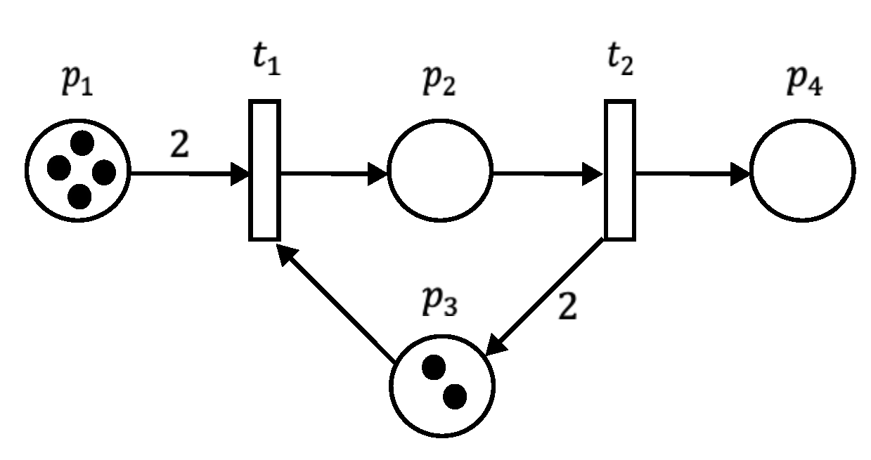
An ordinary PN, or simply PN, is a bipartite graph consisting of two sets of nodes:

P = {p_{1}, p_{2}, \dots, p_{r}}

, and transitions

T = {t_{1}, t_{2}, \dots, t_{s}}

, such that

P \cap T = \emptyset

. These nodes are connected by a set of directed arcs

F \subseteq {(P \times T) \cup (T \times P)}

. Places may represent activities or conditions in systems modeling, whereas transitions represent the occurrence of a condition or the execution of an activity [58]. Figure 1 shows a typical example of a PN model, where circles represent places and rectangles represent transitions, respectively. Each arc carries a number or arc weight, defined by the function

W : F \to N^{+}

, which helps simulate the system’s dynamics. Moreover, a particular state of the system is represented by a distribution of tokens (black dots) within the places, resulting in the marking of the PN. Formally, a marking is defined by the function

M : P \to N

. A marked place means that the corresponding activity or condition is being executed.

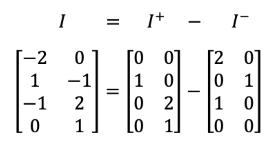
The dynamics or evolution of PN markings involves removing and adding tokens when a firing occurs. Let ^•

t

and

t^{•}

denote the sets of input and output places of transition t. If

M (p) \geq W (p, t)

for each

p \in^{•} t

at some marking M, then the transition t is enabled and can be fired. When transition t is fired,

W (p, t)

tokens are removed for each

p \in^{•} t

, and

W (t, p)

tokens are added to each output place

p \in t^{•}

. The dynamics of a PN can also be described by matrix operations using Equation (6), known as the state equation where

M_{k}

is an

r \times 1

vector representing the current state or marking of the PN, and

M_{0}

is the initial marking or state of the PN.

I

is the incidence matrix of size

r \times s

, given by Equation (7) where

I^{+}

and

I^{-}

are the input and output incidence matrices, respectivily.

M_{k + 1} = M_{k} + Iu

(6)

I = I^{+} - I^{-}

(7)

Each entry of

I^{+}

corresponds to the weights

W (t, p)

, while in

I^{-}

the entries correspond to the weights

W (p, t)

, as illustrated in Figure 2. Finally,

u

is the firing vector of size

s \times 1

, where one entry is 1 (indicating the transition to be fired at marking

M_{k}

), and the remaining entries are zero. Typically, from a set of enabled transitions at a marking

M

, one transition is fired at a time to explore the possible states that can be reached from that marking. This is represented by the notation

M \overset{t}{\to} M^{'}

, where t is the fired transition and

M^{'}

is the marking reached from

M

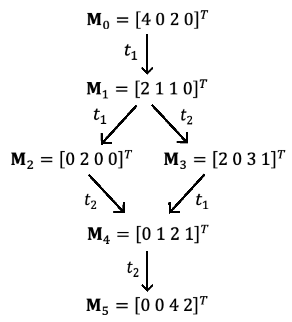
Given a PN with an initial marking

M_{0}

, a firing path

σ

is a sequence of transitions fired from

M_{0}

to marking

M^{'}

, denoted as

M \overset{σ}{\to} M^{'}

. When this occurs,

M^{'}

is said to be reachable from

M_{0}

. The set of all possible reachable markings from

M_{0}

can be represented by a reachability tree, provided that this set is finite. An example of a reachability tree, corresponding to the PN in Figure 1, is shown in Figure 3. Taking the marking

M_{0}

as the root of the reachability tree, a new branch is created for each transition fired from

M_{0}

. After exhausting all possible firings from

M_{0}

, a new level of markings is created, such as

M_{1}

in Figure 3. At the new level, for each marking, new branches are created using the same procedure. When all the possible markings have been obtained, a new level is added to the tree. The process is repeated for each of the markings at every new level until all the reachable markings from

M_{0}

have been obtained. However, when no transition can be fired from a specified marking, it is considered a dead marking. If the evolution of markings is stopped by dead markings without reaching a desired final marking, the PN is blocked.

It should be noted that although the set of reachable markings from

M_{0}

can be finite, the number of these markings could be so large that it becomes impossible to enumerate or represent them using a reachability tree. This issue is known as the state explosion of PN.

3.2. Filtered Beam Search Algorithm

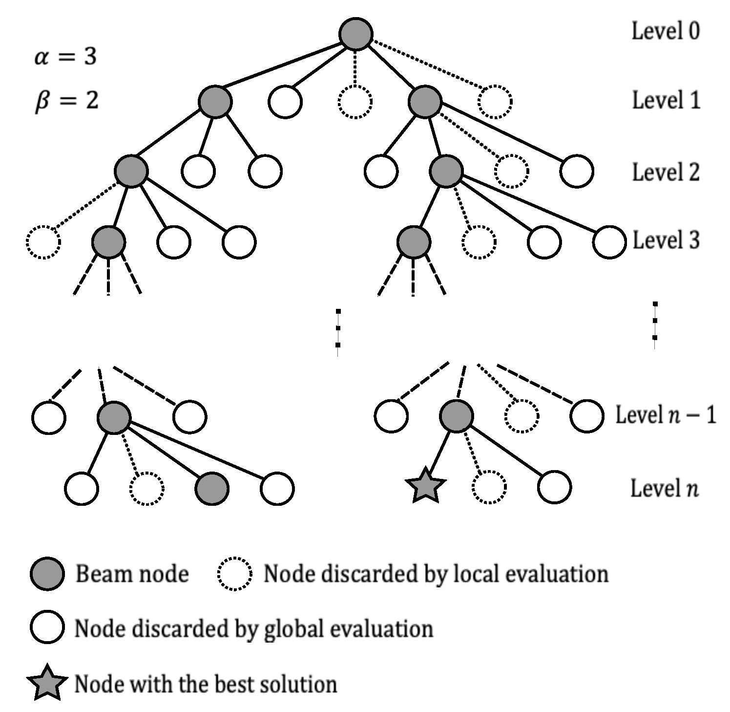
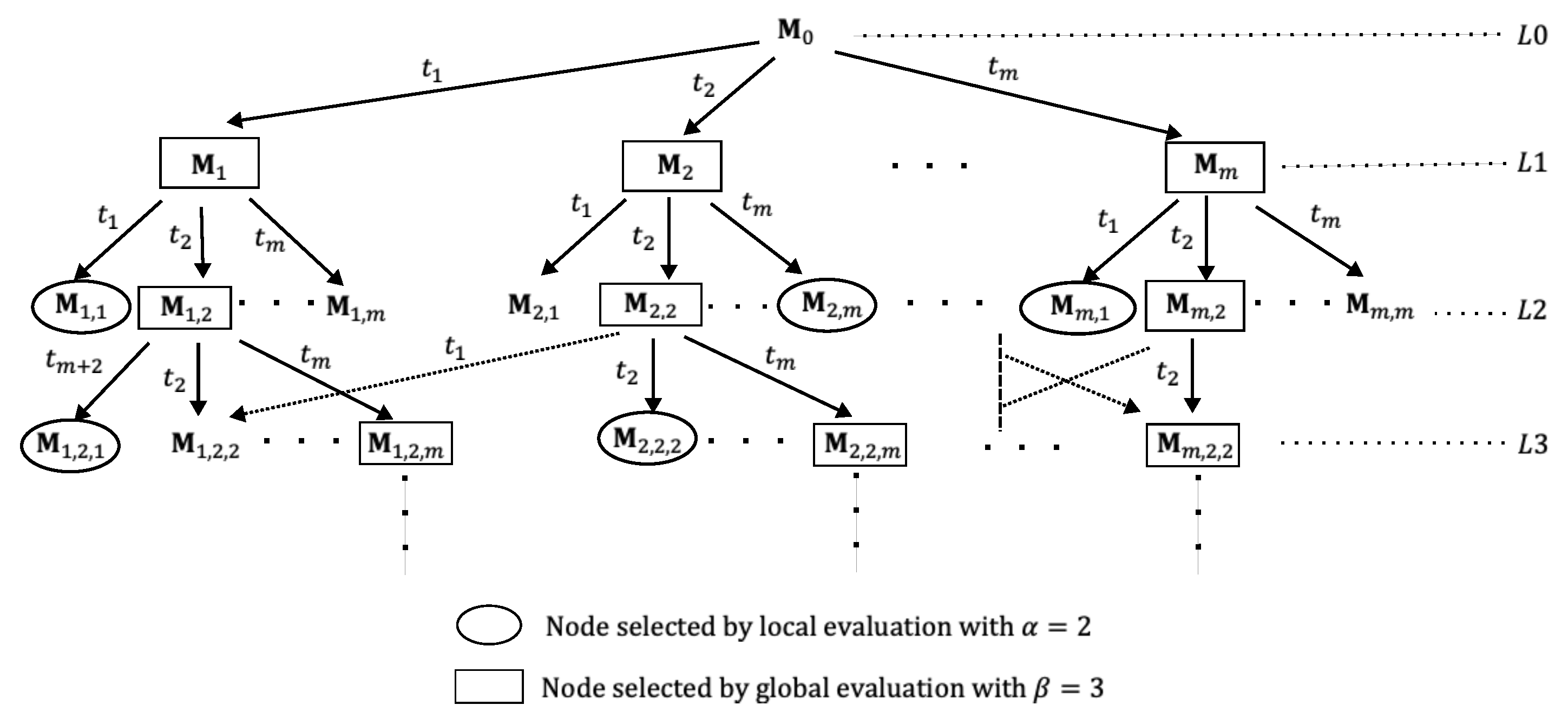
The beam search algorithm was first used as an artificial intelligence technique for speech recognition. It has since been applied to combinatorial optimization problems, such as scheduling problems [59], the travelling salesman problem [60,61,62], and cutting and packing problems [63,64,65]. This method is efficient because solutions to these problems can be constructed sequentially by appending the next operation, city, or item to the partial solution based on the cost it adds. Thus, the construction of the solution can be viewed as a decision tree. At each level, the corresponding nodes represent partial solutions with given costs, while at the last level, the nodes represent complete solutions. One of these complete solutions is then selected as the best or optimal solution. The beam search algorithm performs a breadth-first search followed by a depth-first search. At each level of the tree, the nodes are branched, and those that are not promising for further branching based on a cost function evaluation are pruned. The number of nodes

β

that are branched at each level are the beams. Once these nodes have been selected, the others are discarded permanently. Since the beam search has no backtracking, it is possible to discard good solutions, but it saves much computational effort. In [66], a modification to the beam search was introduced known as the filtered beam search algorithm. As the name suggests, at each level, a local evaluation is carried out over the nodes that share the same parent node. Only those nodes that satisfy a local evaluation condition are considered beam nodes, thereby filtering the nodes. Once all the filtered nodes have been obtained from the parent nodes, only those that satisfy a global evaluation condition become the new beam nodes or parent nodes for the next level.

The number of filtered nodes

α

(filter width) and the number of beam nodes

β

(beam width) are user-defined. However, it is known that larger values require more computational effort to search the tree, while smaller values reduce the likelihood of finding the best or optimal solution. A representation of the filtered beam search algorithm is shown in Figure 4 for a solution with a sequence of n nodes. Sometimes, it is desired to maintain diversity in the search by setting

α < β

, which guarantees that at least one beam node is selected from a different parent node [64].

4. PN-Based Algorithm for Solving the 1D-CSP

In this section, we first provide details about the PN model used to construct solutions for a given instance of the 1D-CSP. Next, we explain how the beam search algorithm, based on the reachability tree, is used to find the best solution.

4.1. PN Model for the 1D-CSP

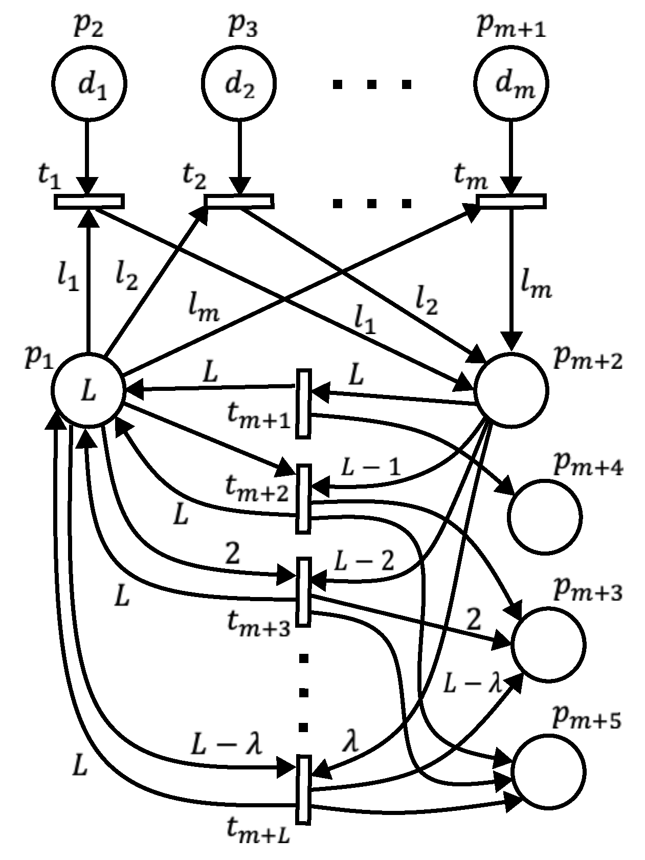
As mentioned above, we use ordinary PN to model a given instance of the 1D-CSP. Figure 5 illustrates the general PN model for a given instance of the 1D-CSP, with m different items and stock length L. The construction of a solution for a 1D-CSP instance through the PN model follows the next-fit heuristic principle. This means that items are added sequentially to the solution as long as the total length of the items, or pattern length, does not exceed the length of the stock. Otherwise, the next item is put into a new stock, and the process is repeated until all items have been added to the solution. In this way, there will be patterns with or without waste, and the total waste of the solution will be the sum of the waste yielded from each pattern. The PN model allows the formation of patterns with and without waste, enabling the beam search algorithm to find the solution with the minimum waste and the minimum number of stocks with waste.

According to the general PN model, there will be m places for each item type labeled

p_{2}, p_{3}, \dots p_{m + 1}

, as shown in Figure 5. We refer to these places as item places. The number of tokens inside the item places represents the number of orders of each item, denoted

d_{1}, d_{2}, \dots, d_{m}

. The stock is represented by a single place labeled

p_{1}

, and the number of tokens inside this place is equal to the stock length, L. We refer to this place as the stock place. Item places, as well as the stock place, are input places for transitions

t_{1}, t_{2}, \dots, t_{m}

, referred to as item transitions. Each item transition consumes a token from its corresponding item place, indicating that an order of that item is being put into a solution. Similarly, each item transition removes

l_{i}

tokens from the stock place, which corresponds to the length of the item of the corresponding item place. As items are taken, a pattern is formed, and its length is accumulated in the place labeled

p_{m + 2}

, which we name the pattern place. As shown in Figure 5, the pattern place is an output place of each item transition, where each one adds

l_{i}

tokens to the pattern place according to the item length it is being added to the solution. Therefore, the number of tokens inside the pattern place varies from 0 to L. However, the minimum pattern length will be

λ = m i n {l_{1}, l_{2}, \dots, l_{m}}

, representing a pattern formed by only one order of the item with the smallest length.

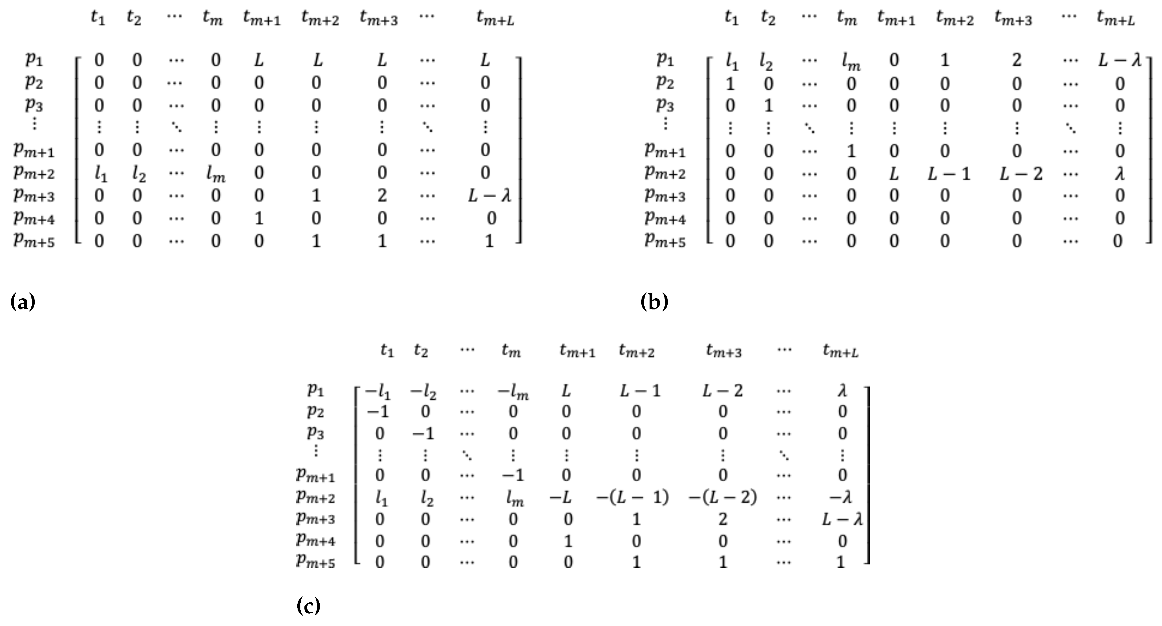
The transitions

t_{m + 1}, t_{m + 2}, t_{m + 3}, \dots, t_{m + L}

are the pattern transitions, and there will be L transitions of this type. A pattern transition removes tokens from the pattern place according to the corresponding pattern length that has been formed. For example,

t_{m + 1}

removes L tokens,

t_{m + 2}

removes

L - 1

tokens, and so on, such that

t_{m + L}

removes

λ

tokens. Since a pattern includes the lengths of the items as well as the unused material of the stock (if any), pattern transitions

t_{m + 2}, t_{m + 3}, \dots, t_{m + L}

are output transitions of the stock place to complete the pattern formation. Thus,

t_{m + 2}

removes one token,

t_{m + 3}

removes two tokens, and so on, such that

t_{m + L}

removes

L - λ

tokens from the stock place. Transition

t_{m + 1}

is not an output transition of the stock place since it corresponds to a pattern without waste. At the same time, the pattern transitions are input transitions of the stock place so that once a pattern has been formed and included in a solution, another stock must be available to continue the process of forming the solution. Each pattern transition adds L tokens to the stock place as shown in Figure 5. So far, the PN model can construct any possible solution by starting with any item, but we included three more places to enhance the model. These places are

p_{m + 3}

p_{m + 4}

and

p_{m + 5}

, where

p_{m + 3}

records the amount of waste,

p_{m + 4}

helps to count the number of stocks without waste, and

p_{m + 5}

counts the number of stocks with waste. Places

p_{m + 3}

and

p_{m + 5}

are output places of the pattern transitions. Each pattern transition adds one token to

p_{m + 5}

while

p_{m + 3}

receives

1, 2, \dots, L - λ

tokens from transitions

t_{m + 2}, t_{m + 3}, \dots, t_{m + L}

, respectively. Place

p_{m + 4}

is an output place of transition

t_{m + 1}

, which adds one token each time there is a pattern without waste. Based on the above descriptions, Figure 6 shows the general form of the incidence matrices of the PN model for an instance of the 1D-CSP.

4.2. Marking Evolution and Solution Construction

To obtain a solution for a given instance of the 1D-CSP with the PN model described in the previous section, referred to as PN-CSP, we begin with the initial marking as shown in Figure 5 where there is an unused stock (place

p_{1}

) and m items with their corresponding number of orders (places

p_{2}

p_{m + 1}

). Hence, the general form of the initial marking of the PN-CSP is:

M_{0} = {[L d_{1} d_{2} \dots d_{m + 1} 0 0 0 0]}^{T} .

From the initial marking, the enabled transitions are

t_{1}, t_{2}, \dots, t_{m}

so that any of the items could be the first in the solution. The solution is constructed in a linear sequence of items arranged from left to right. Once an enabled transition is fired, the pattern place accumulates tokens representing the length of the item placed first in the solution. Suppose transition

t_{2}

is fired; then the resulting marking is:

M_{1} = {[L - l_{2} d_{1} d_{2} - l_{2} \dots d_{m + 1} l_{2} 0 0 0]}^{T} .

While the number of tokens in

p_{m + 2}

is not equal to or greater than any of the weights of the arcs

L, L - 1, L - 2, \dots λ

, transitions

t_{1}, t_{2}, \dots, t_{m}

can be fired one at a time because they will be the only ones enabled. This means the pattern formation continues as long as there is space in the current stock. However, if a determined pattern length less than the stock length is reached, such as

L - 1, L - 2

, or

λ

, the corresponding transition from

t_{m + 2}

t_{m + L}

is enabled, considering there will be

1, 2,

L - λ

tokens in place

p_{1}

, representing the waste of the stock. If one of the transitions

t_{m + 2}, \dots, t_{m + L}

is selected to be fired, the pattern formation stops to renew the stock for a new pattern. For example, consider the marking:

M_{k} = {[2 a b \dots c L - 2 0 0 0]}^{T}

where

a, b, \dots, c

are the corresponding remaining number of items’ orders after

k - 1

items have been included in the first pattern of the solution, and

M_{k} (p_{m + 2}) = L - 2

. Then

t_{m + 3}

is enabled and can be fired, yielding the marking:

M_{k + 1} = {[L a b \dots c 0 2 0 1]}^{T} .

Here, there is a new empty stock of length L, and one stock with waste (

M_{k + 1} (p_{m + 5}) = 1

) has been generated as part of the solution with a waste of 2 (

M_{k + 1} (p_{m + 3}) = 2

). With the new empty stock, the construction of the solution continues with the remaining items’ orders. When a pattern transition is fired, it means that a cutting pattern has been formed, adding a new stock with or without waste to the solution. These markings that enable and fire a pattern transition are called pattern markings. On the other hand, if an item transition is fired, it means that an item has been added to the current pattern in construction. These markings that enable and fire an item transition are called item markings. The marking evolution is performed as described, forming patterns and renewing the stocks when needed until all of the items have been included in a solution.

When the number of tokens in places

p_{2}, p_{3}, \dots, p_{m + 1}

is zero, the solution has been completed, and the marking

M_{f} = {[L 0 0 \dots 0 0 ω ν η]}^{T}

is considered the final marking, where

ω

is the final total waste,

ν

is the final number of stocks without waste, and

η

is the final number of stocks with waste. Therefore, the solution can be obtained with the firing sequence

σ

obtained from

M_{0}

M_{f}

, that is

M_{0} \overset{σ}{\to} M_{f}

. A final firing sequence would have the following form:

σ = t_{2}, t_{m}, \dots, t_{1}, t_{m + 3}, t_{1}, t_{3}, \dots, t_{m}, t_{m + 1}, \dots, t_{m + L}, t_{m}, t_{1}, \dots, t_{3}, t_{m + 2} .

To decode

σ

into a sequence of item lengths, the pattern transitions

t_{m + 3}

t_{m + 1}

t_{m + L}

and

t_{m + 2}

are dropped, and a new sequence is made up with the remaining transitions. This new sequence is:

ς = t_{2}, t_{m}, \dots, t_{1}, t_{1}, t_{3}, \dots, t_{m}, \dots, t_{m}, t_{1}, \dots, t_{3} .

The solution is formed with either the weights

W (t_{i}, p_{m + 2})

W (p_{1}, t_{i})

for

1 \leq i \leq m

for each of the transitions in

ς

, such that these weights correspond to the lengths of the items. Therefore, for the final firing sequence

σ

, the solution would have the following form:

s = l_{2}, l_{m}, \dots, l_{1}, l_{1}, l_{3}, \dots, l_{m}, \dots, l_{m}, l_{1}, \dots, l_{3} .

5. Filtered Beam Search Algorithm Implementation

Consider the reachability tree construction of the PN-CSP with initial marking

M_{0} = {[L d_{1} d_{2} \dots d_{m + 1} 0 0 0 0]}^{T}

for a given instance of the 1D-CSP. Starting from this initial marking, all potential solutions are derived by investigating firing sequences leading to the final marking

M_{f} = {[L 0 0 \dots 0 0 ω ν η]}^{T}

. However, exhaustive exploration of all sequences is computationally intensive. To solve this issue, we use the FBS, which reduces explored markings as we progress in the reachability tree. FBS does not perform backtracking like traditional any-time search methods, optimizing computational efficiency. The effectiveness of FBS depends on parameters

α

and

β

, chosen to balance exploration and exploitation. Algorithm 1 outlines our FBS implementation, starting by generating all child nodes from firing transitions

t_{1}, t_{2}, \dots, t_{m}

at the initial marking or the root node (level 0 or

L 0

), resulting in m markings at level 1 (

L 1

), as shown in Figure 7. In our FBS, each marking at L1 is neither locally nor globally evaluated, treating each node as a potential beam node, contrary to [59]. We made this decision because, by the local evaluation, the algorithm will tend to select the solutions with the largest items placed first, minimizing waste in the initial stock. Preliminary experiments showed this approach yields better solutions compared to selecting only

β

nodes at

L 1

. Thus, starting from L2, we apply both local and global evaluations, setting

α \leq β

to ensure solution diversity.

In most beam search algorithm implementations, node costs at any node are computed using a function that considers cumulative costs up to the node and an estimation of the remaining solution’s cost. The effectiveness of these algorithms heavily depends on choosing the right estimation cost function. Usually, in the FBS algorithm, local evaluation uses cumulative costs, while global evaluation considers both cumulative and estimated costs. Our FBS implementation employs the bi-objective function (1) as a fitness function to perform both local and global evaluations. This function calculates the complete solution, capturing the number of stocks used, the total waste generated, and the number of stocks with waste that have been generated in the solution.

As we progress in constructing the reachability tree, each node or marking represents only a partial solution, thus its corresponding cost is also partial. Despite not having a complete solution, partial solutions provide insights into the number of stocks used, those with or without waste, and the amount of unused material or potential waste on the current stock. For example, at the initial marking or root node, no stock has been used, resulting in no stocks with or without waste, and an unused material length of L. At level L1, item markings represent solutions where one order of each item has been taken, but no stock has been fully utilized with or without waste. Eventually, as the reachability tree progresses, pattern markings are reached at some level, indicating that a cutting pattern has been obtained. At the first pattern marking, a stock has been used, and the waste amount for the stock is known. Subsequent item markings’ costs must consider the used stock and its waste. It can be seen from the bi-objective function (1) that the first term sums the partial wastage of each used stock, while the second sums the number of stocks with waste. We compute two cumulative costs accordingly: one for waste using Equation (8) and another for the number of stocks with waste using Equation (9). Both are employed in Equation (10) for the global evaluation of nodes. These two cumulative costs are computed upon reaching a pattern marking, while Equation (11) is utilized for local evaluations, considering the unused material of the current stock in each solution.

W_{w} = W_{w} + \sqrt{\frac{w_{j}}{L}}

(8)

W_{s w} = \frac{M (p_{m + 5})}{M (p_{m + 5}) + M (p_{m + 4})}

(9)

F_{g l o b a l} = \frac{W_{w} + W_{s w}}{M (p_{m + 5}) + M (p_{m + 4}) + 1}

(10)

\begin{matrix} F_{l o c a l} & = \{\begin{matrix} \frac{1}{M (p_{m + 5}) + M (p_{m + 4}) + 1} (\frac{M (p_{1})}{L} + W_{s w}) & if M is an item marking . \\ \frac{1}{M (p_{m + 5}) + M (p_{m + 4}) + 1} (\frac{w_{j}}{L} + W_{s w}) & if M is a pattern marking . \end{matrix} \end{matrix}

(11)

In Equations (8) and (11),

w_{j}

is obtained from the incidence matrix of PN-CSP, where

w_{j} = I (p_{m + 3}, t)

for

t \in {t_{m + 2}, t_{m + 3}, \dots, t_{m + L}}

. This is because when a pattern transition is fired, the marking of place

p_{1}

is immediately updated to L, indicating that the amount of waste in the already used stock is lost. However, this amount of waste can be determined from the incidence matrix. The cumulative costs

W_{w}

and

W_{s w}

are set to zero for the item markings between the initial marking and the first pattern marking. These costs are computed and updated at each reached pattern marking. Consequently, the outcomes of

W_{w}

and

W_{s w}

are retained for the item markings between two subsequent pattern markings. Once the final marking is reached, the last

F_{g l o b a l}

outcome is set as the best solution

F_{b e s t}

. To determine whether the final marking has been reached, at each level, we compare the markings obtained with the desired final marking

M_{f} (p_{1})

. However, we only consider the marking of places

p_{1}, p_{2}, \dots, p_{m + 2}

. Specifically, we compare the marking

M = [M (p_{1}) M (p_{2}) M (p_{3}) \dots M (p_{m + 1}) M (p_{m + 2}) * * *]

, obtained at some level, with the final marking

M_{f} = [L 0 0 \dots 0 0 * * *]

. The ’*` means that the marking of the corresponding places is not considered for the comparison. This is because we do not know in advance how much waste would be generated by the best solution or the number of stocks with and without waste. However, we know that at the final marking, there are no more item orders to place, and the last stock is generated when the last item order is taken for the final cutting pattern.

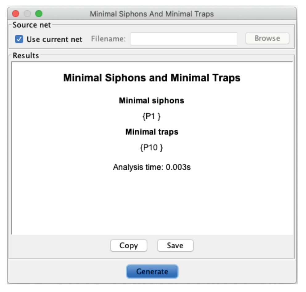
Observe from Algorithm 1, lines 17 and 29, that when performing global and local evaluations, we do not necessarily select

β

α

number of markings, respectively. Instead, we select the minimum value between

β

(or

α

) and the number of markings obtained globally (or locally). This is because, in a reachability tree, a marking could be generated by firing different transitions, resulting in fewer markings than the

β

markings needed at a level or fewer than the

α

markings needed from a parent marking or beam node. In some beam search algorithm implementations, if the required

β

nodes are not met for some level, then more parent nodes at the previous level are explored to meet the required

β

nodes. However, we do not do this in our FBS implementation, as it is possible to encounter dead markings. This might make it impossible to complete the required number of nodes. Dead markings are related to the liveness property of a PN and this property is closely related to the presence of siphons [67]. It is known that a PN with siphons is likely to be non-live, as once the places of a siphon become unmarked at some marking, they remain unmarked in all subsequent markings. We performed a structural analysis for an instance with ten different items and a total of 20 orders, using an open-source PN modeling platform called PIPE2 version 4.3.0 [68] to determine the presence of siphons. The results are shown in Figure 8, indicating that place

p_{2}

(

p_{1}

according to the enumeration of the PIPE2 platform) is a minimal siphon. Extending this result for the general PN-CSP model with the initial marking in the general form, and considering the dynamics described in the above paragraphs, places

p_{1}, p_{2}, \dots, p_{m}

could be minimal siphons and could become unmarked at some marking. The PN-CSP would become deadlocked if all the places

p_{1}, p_{2}, \dots, p_{m}

are unmarked, although this situation indicates that the desired final marking has been reached. However, to prevent our algorithm from getting stuck due to incomplete

β

nodes at some levels and potentially failing to reach the desired final marking, we decided to use the minimum number of nodes as outlined in Algorithm 1.

Algorithm 1 Pseudocode of algorithm FBS-PN-CSP

Input:: Number of different item types (m), stock length (L), item lengths $(l_{1}, l_{2}, \dots, l_{m})$ , and item orders $(d_{1}, d_{2}, \dots, d_{m})$ .
Output:: $F_{b e s t}$
1:: With the instance data, generate the incidence matrices $I^{+}$ , $I^{-}$ and obtain the incidence matrix $I$ .
2:: Generate the initial marking as $M_{0} = [L d_{1} d_{2} \dots d_{m + 1} 0 0 0 0]$ .
3:: Set the beamwidth $β$ and the filterwidth $α$ .
4:: $F_{b e s t} \leftarrow \infty$
5:: $W_{w} \leftarrow 0$
6:: $W_{s w} \leftarrow 0$
7:: Generate level $L 0$ of the reachability tree with the marking $M_{0}$ as the root node such that $C u r r e n t l e v e l = {M_{0}}$ .
8:: $l e v e l \leftarrow 0$
9:: $B e s t s o l u t i o n \leftarrow F a l s e$
10:: while $B e s t s o l u t i o n i s F a l s e$ do
11:: for each marking in $C u r r e n t l e v e l$ do
12:: Get $W_{w}$ , $W_{s w}$ and $F_{g l o b a l}$ .
13:: end for
14:: if level > 1 then
15:: Kept the $μ = \min (β, | C u r r e n t l e v e l |)$ best markings in $C u r r e n t l e v e l$ with the lowest $F_{g l o b a l}$ cost and form the set $B$ with these markings. Eliminate the remaining markings from $C u r r e n t l e v e l$ .
16:: else
17:: Kept the $μ = | C u r r e n t l e v e l |$ markings in $C u r r e n t l e v e l$ and form the set $B$ with these markings.
18:: end if
19:: $N e w l e v e l = \emptyset$
20:: for each marking $M$ in $B$ do
21:: Determine the reachable markings $M^{'}$ from $M$ with Equation (6) and form the set $M_{r}$ with those reachable markings, where $r = 1, 2, \dots, | B |$ .
22:: if $M_{r} \neq \emptyset$ then
23:: Obtain $W_{w}$ , $W_{s w}$ , $F_{l o c a l}$ and $F_{g l o b a l}$ for each $M^{'} \in M_{r}$ .
24:: if level >0 then
25:: Check whether any marking $M^{'} \in M_{r}$ has already been generated previously. If it has, let $M_{p r e v}^{'} \in M_{1} \cup M_{2} \cup \dots \cup M_{r - 1}$ be the previously generated marking that is equal to $M^{'} \in M_{r}$ , and then eliminate from the reachability tree the one with the maximum $F_{g l o b a l}$ cost.
26:: if $M_{r} \neq \emptyset$ then
27:: Kept the $τ = \min (α, | M_{r} |)$ markings with the lowest $F_{l o c a l}$ cost and eliminate the remaining ones from $M_{r}$ .
28:: end if
29:: else
30:: Keep the markings in $M_{r}$ .
31:: end if
32:: Make $N e w l e v e l \cup M_{r}$
33:: end if
34:: end for
35:: Check whether the final marking $M_{f} = [L 0 0 \dots 0 0 * * *]$ has been reached.
36:: if $M_{f}$ has been reached then
37:: $F_{b e s t} \leftarrow F_{g l o b a l}$
38:: $B e s t s o l u t i o n \leftarrow T r u e$
39:: else
40:: $l e v e l \leftarrow l e v e l + 1$
41:: $C u r r e n t l e v e l = N e w l e v e l$
42:: end if
43:: end while

6. Experiments

Although we identified a wide variety of datasets in the literature, most studies do not use common datasets or performance measures to compare the algorithms. Additionally, implementing the published algorithms correctly can be challenging, and often, the code is not shared. Nevertheless, we identified two algorithms that share some similarities with our algorithm and are not based on populations. These algorithms were tested on five datasets that we found suitable for comparison with our algorithm. The first algorithm is the Least Lost Algorithm (LLA), introduced in [54], which uses a dataset of ten instances with a single stock size. We refer to this dataset as hinterding because, to the best of our knowledge, it was first used in [35]. The LLA is executed in two phases. In the first one, the item lengths are arranged in decreasing order while in the second, the second half of the arrangement is put before the first half. In both phases, the items are taken from the arrangement to construct cutting patterns by beginning with those that have no waste. If no additional cutting patterns without waste can be found, the search continues with patterns that have one unit of waste. This process continues by increasing the allowed waste by one unit until all the item orders have been included in a cutting pattern. If the number of stocks used is above the optimal theoretical value by more than 5%, the algorithm performs the second phase. The feature of increasing the allowed waste by one unit is represented in our PN-CSP model with the pattern transitions. The LLA was compared to the EP algorithm shown in [8] over the same dataset and the LLA yielded better results.

The other algorithm we compare to the FBS-PN-CSP is the Generate & Solve algorithm (G&S) presented in [55]. This algorithm is also executed in two phases. The first one reduces the problem size using a tree method that constructs all possible cutting patterns. Feasible cutting patterns are then selected and sent to the second phase, where an integer linear programming (ILP) method is implemented to obtain the best solution for the reduced set of solutions. In the first phase, a new reduced set of solutions is generated by considering an aging mechanism for previously used solutions, which can be re-selected as long as they have not reached a specified age limit. These new solutions are then sent to the second phase to determine the best solution among them, replacing the older solution if the new one is better. This process continues until a predefined time limit is reached, and the last solution found is returned as the best solution for the problem. The G&S algorithm was compared to the column generation technique. Both algorithms performed similarly for small instances, but the G&S algorithm was more effective for large instances. From the datasets used in [55], we selected the ones called hard28, hard10, and wae_gau1, available at [69]. Additionally, we included the dataset falkenauer_U from the same repository, which consists of four groups named binpack1, binpack2, binpack3, and binpack4. Table 1 provides details about the datasets. The third column lists the minimum and maximum number of item types among the instances of each dataset, while the fourth column shows the number of different item types, along with the standard deviation in rounded brackets. Both the hinterding dataset and the hard10 dataset have four different item types, but the variability in the former is greater than in the latter.

The comparisons among the three algorithms were made with respect to the number of stocks used and its optimal theoretical value, which can be obtained using Equation 12. The experiments were conducted on a Quad-Core Intel^(R) Core^(TM) i5 computer with a 3.4 GHz processor and 8 GB RAM. All three algorithms were coded in Python 3.11.1. For the second phase of the G&S algorithm, we used the Scipy package with the linprog library. We also set the same parameter values as in [55], that is, specifically: a time limit of 600 seconds for the G&S algorithm, a mutation rate of 10%, a maximum age of 2, and a maximum number of cutting patterns for the tree construction of 1,000,000. Additionally, we also executed the G&S algorithm 10 times for each instance. However, we did not set a time limit in the second phase of the G&S algorithm, as the solutions from the ILP solver were obtained in an acceptable time.

l b = ⌈\frac{\sum_{i}^{m} l_{i} d_{i}}{L}⌉

(12)

One of the issues with beam search algorithms is the selection of the beam width

β

. The smaller the

β

value, the faster the search, but this comes at the loss of optimality due to aggressive pruning. We conducted preliminary experiments to determine suitable

β

and

α

values, considering the condition

α \leq β

. These experiments were carried out with the hinterding dataset. In all ten instances of this dataset, we observed that the best solutions were found with a beam width between 5 and 25; with higher values, the solution improvement was negligible. Thus, for all the experiments with the FBS-PN-CSP algorithm, we used the interval

5 \leq β \leq 35

for the beam width, at steps 5, 15, 25, and 35, with

2 \leq α \leq β

for each value of

β

. However, for the hinterding dataset, we additionally implemented a

β

value of 45, and for the hard10 dataset, we only could implement a beam width of

β = 5

. With

α = 1

, no good solution was found in any instance.

7. Results

Table 2, Table 3, Table 4, Table 5, Table 6, Table 7, Table 8 and Table 9 show the best results obtained with each algorithm for the number of stocks used and the time taken. Additionally, we provide the

l b

value for all the instances and the percentage above this value (%

> l b

) obtained by each algorithm. The FBS-PN-CSP, G&S, and LLA algorithms were compared only with the hinterding and falkenauer_U datasets since the LLA algorithm ran out of memory for the other datasets. The minimum value of stocks used among the compared algorithms is highlighted in boldface. For the G&S algorithm, we provide the best solution found within the 10 executions, and likewise, for the FBS-PN-CSP algorithm, we include the best combinations of beam width and filter width where the best stock result was found.

For the hinterding dataset, the three algorithms obtained the same optimal theoretical value for the 1a-5a instances and the 7a instance. The FBS-PN-CSP and the G&S algorithms also obtained the same best result for the 6a instance. Only the G&S had the optimal theoretical value for the 8a-10a instances. The FBS-PN-CSP algorithm had better results than the LLA algorithm for the 6a, 8a, and 9a instances, while for the 10a instance, both had the same result. Although the FBS-PN-CSP algorithm was not better than the G&S algorithm for instances 8a-10a, it obtained a percentage above the optimal theoretical value of less than 1%. The FBS-PN-CSP algorithm was more efficient than the G&S algorithm in 6 out of 7 instances where they are equal, namely 2a-7a. However, the LLA algorithm had better times in all the instances where it had the same results as the other two algorithms. The beam width of the FBS-PN-CSP algorithm seems to increase as the number of items and the stock length increase. The highest beam width and filter width values were obtained in the 10a instance, which has the higher number of items and the longest stock.

The results of the FBS-PN-CSP and G&S algorithms are shown in Table 3 for the hard28 dataset. Both algorithms obtained the same best results except for the BPP900 and BPP781 instances, where the FBS-PN-CSP had the better results. Nevertheless, neither obtained the optimal theoretical value. The FBS-PN-CSP was more efficient in 15 out of 27 instances where both algorithms obtained the same result. As for the beam width of the FBS-PN-CSP, this was the minimum value of the tested values, that is,

β = 5

for all the instances. For the hard10 instances, the G&S algorithm was better than the FBS-PN-CSP algorithm as shown in Table 4. However, the G&S algorithm only had the optimal theoretical value in one instance, namely HARD9. Even with the smaller value of the beam width, the time required for the FBS-PN-CSP was far higher than the time of the G&S algorithm. For this reason, we could not implement larger values for the beam width since the computational cost was prohibited, although it did not run out of memory. Despite the results for stock used by the FBS-PN-CSP algorithm, it was not far from those of the G&S and could be at least equal if higher values of the beam width can be implemented.

In 12 out of 17 instances of the waegau1 dataset, the FBS-PN-CSP algorithm matched the best results of the G&S algorithm (Table 5), and in 9 of these 12 instances, it had better times. In 4 out of the 17 instances, the FBS-PN-CSP had better results, and only in one instance, the G&S was better than the FBS-PN-CSP. In 7 out of the 17 instances, the FBS-PN-CSP obtained the optimal theoretical value, while the G&S did so in only four instances. Regarding beam width, four instances required the higher tested values, namely 25 and 35, but with a small filter width.

Table 6 shows the best stock results for the binpack1 instances of the falkenauer_U dataset, where the FBS-PN-CSP, G&S, and LLA algorithms are compared. The FBS-PN-CSP and the G&S algorithms obtained the optimal theoretical values of each instance, but the FBS-PN-CSP had the best times. The LLA algorithm achieved the optimal theoretical values in 12 out of 20 instances and had better times than the FBS-PN-CSP algorithm. Only in two instances did the FBS-PN-CSP use the higher beam width values (25 and 35), but in most instances, the value was 5, which is the smallest value tested. For the binpack2 instances, the FBS-PN-CSP had the same results as the G&S algorithm in 19 instances (Table 7), and these were equal to the corresponding optimal theoretical values. All the results of the G&S algorithm were equal to the optimal theoretical value. The LLA algorithm had the optimal theoretical values in half of the instances and the best times among the three algorithms. The FBS-PN-CSP algorithm had better times than the G&S in ten of the instances where they had the same stock result. The beam width was mostly 15 throughout the binpack2 instances. The binpack3 results (Table 8) show that the G&S algorithm obtained the optimal theoretical values in all instances, and the FBS-PN-CSP algorithm did so in 17 instances. Likewise, the LLA algorithm achieved this in only 11 instances, but with better times than the FBS-PN-CSP and G&S algorithms. Only in the instance u500_14 did the FBS-PN-CSP obtain a better time than the G&S algorithm. The values of the beam width were 15 and 25 in most instances, and the filter value was higher than in the previous groups of instances of the falkenauer_U dataset. Similar results were obtained for the binpack4 instances shown in Table 9, where the G&S algorithm outperformed the other two algorithms. In all instances, this algorithm obtained the optimal theoretical value, the FBS-PN-CSP did so in 14 instances, and the LLA algorithm in 7 instances, but only with better times than the FBS-PN-CSP. The beam width was mostly higher, namely 25 throughout the instances, as was the filter width. Although in the instances of binpack2, binpack3, and binpack4 the FBS-PN-CSP was not better than the G&S in terms of the number of stocks used, the percentage above the optimal theoretical values was less than 1% with a difference of one stock in all cases.

8. Discussion

It can be observed from the results shown in the previous section that the FBS-PN-CSP algorithm is effective and efficient in most of the instances it was tested in comparison with the other two algorithms, except for the hard10 dataset. It must be taken into account that the G&S algorithm had a time limit for its execution of 600 seconds. The FBS-PN-CSP best results were obtained below such time in only one execution. Additionally, the average time from 10 executions of the G&S was longer than the FBS-PN-CSP algorithm and the LLA algorithm in most instances. On the other hand, the LLA algorithm had the best times compared to the FBS-PN-CSP and G&S algorithms, but the number of stocks used was of lower quality. We have observed that the computational time for the FBS-PN-CSP for longer stocks tends to be higher due to the PN model structure. As the stock gets longer, the number of pattern transitions increases considerably. This observation can be noted for the hard10 dataset, which has the longest stock among the datasets tested. Moreover, the beam width tends to increase as well as the computational time, as both the number of item types and the number of orders increase. Except for the hard10 dataset, in those instances where the FBS-PN-CSP algorithm did not obtain the optimal theoretical value, the solutions were just above this value by one stock.

9. Conclusions

In this paper, an algorithm based on the modeling power of Petri nets was presented for solving the one-dimensional cutting stock problem (1D-CSP). To the best of our knowledge, Petri nets had not been used to address the 1D-CSP. Firstly, we provided the Petri net general model to construct the solutions of a given instance of the 1D-CSP. Each solution consists of a series of cutting patterns with or without waste. Then, the filtered beam search algorithm is used to search for the best solution throughout the exploration of the nodes of the reachability tree. The algorithm, called FBS-PN-CSP, was compared to the Generate & Solve and the Least Lost algorithms over five datasets with a total of 145 instances and shown to be effective and efficient in most of the datasets. Therefore, either with instances of low or high complexity, the FBS-PN-CSP is shown to be competitive. Some enhancements to the Petri model and slight modifications to the algorithm implementation could improve the performance.

Author Contributions

Conceptualization, I.B.-V.; methodology, I.B.-V., J.M.-M, N.H.-R and G.E.A.-F; software, I.B.-V., J.M.-M. and G.E.A.-F.; validation, J.M.-M., N.H.-R and G.E.A.-F.; formal analysis, I.B.-V., J.M.-M. and N.H.-R.; data curation, I.B.-V., N.H.-R. and G.E.A.-F.; writing—original draft preparation, N.H.-R. and G.E.A.-F.; writing—review and editing, I.B.-V. and J.M.-M. All authors have read and agreed to the published version of the manuscript.

Funding

This research received no external funding.

Institutional Review Board Statement

Not applicable.

Data Availability Statement

The original contributions presented in the study are included in the article, further inquiries can be directed to the corresponding author.

Conflicts of Interest

The authors declare no conflict of interest.

References

Garey, M.R.; Johnson, D.S. Computers and Intractability: A Guide to the Theory of NP-Completeness; W. H. Freeman, 1979. [Google Scholar]
Wäscher, G.; Hausner, H.; Schumann, H. An improved typology of cutting and packing problems. European Journal of Operational Research 2007, 183, 1109–1130. [Google Scholar] [CrossRef]
Lee, D.; Son, S.; Kim, D.; Kim, S. Special-Length-Priority Algorithm to Minimize Reinforcing Bar-Cutting Waste for Sustainable Construction. Sustainability 2020, 12. [Google Scholar] [CrossRef]
Vishwakarma, R.; Powar, P.L. An efficient mathematical model for solving one-dimensional cutting stock problem using sustainable trim. Advances in Industrial and Manufacturing Engineering 2021, 3, 100046. [Google Scholar] [CrossRef]
Valério de Carvalho, J. LP models for bin packing and cutting stock problems. European Journal of Operational Research 2002, 141, 253–273. [Google Scholar] [CrossRef]
Delorme, M.; Iori, M.; Martello, S. Bin packing and cutting stock problems: Mathematical models and exact algorithms. European Journal of Operational Research 2016, 255, 1–20. [Google Scholar] [CrossRef]
Machado, A.A.; Zayatz, J.C.; da Silva, M.M.; Melluzzi Neto, G.; Leal, G.C.L.; Palma Lima, R.H. Aluminum bar cutting optimization for door and window manufacturing. DYNA 2020, 87, 155–162. [Google Scholar] [CrossRef]
Liang, K.H.; Yao, X.; Newton, C.; Hoffman, D. A new evolutionary approach to cutting stock problems with and without contiguity. Computers & Operations Research 2002, 29, 1641–1659. [Google Scholar] [CrossRef]
Lee, D.Y.; DiCesare, F. Scheduling flexible manufacturing systems using Petri nets and heuristic search. IEEE Transactions on Robotics and Automation 1994, 10, 123–132. [Google Scholar] [CrossRef]
Huang, B.; Jiang, R.; Zhang, G. Heuristic Search for Scheduling Flexible Manufacturing Systems Using Multiple Heuristic Functions. In Proceedings of the Modern Advances in Applied Intelligence; Ali, M.; Pan, J.S.; Chen, S.M.; Horng, M.F., Eds.; Cham, 2014; pp. 178–187.
Libralesso, L.; Fontan, F. An anytime tree search algorithm for the 2018 ROADEF/EURO challenge glass cutting problem. European Journal of Operational Research 2021, 291, 883–893. [Google Scholar] [CrossRef]
Xu, G.; Chen, Y. Petri-Net-Based Scheduling of Flexible Manufacturing Systems Using an Estimate Function. Symmetry 2022, 14. [Google Scholar] [CrossRef]
Mejía, G.; Niño, K. A new Hybrid Filtered Beam Search algorithm for deadlock-free scheduling of flexible manufacturing systems using Petri Nets. Computers & Industrial Engineering 2017, 108, 165–176. [Google Scholar] [CrossRef]
Parreño, F.; Alonso, M.; Alvarez-Valdes, R. Solving a large cutting problem in the glass manufacturing industry. European Journal of Operational Research 2020, 287, 378–388. [Google Scholar] [CrossRef]
Birgin, E.; Ferreira, J.; Ronconi, D. A filtered beam search method for the m-machine permutation flowshop scheduling problem minimizing the earliness and tardiness penalties and the waiting time of the jobs. Computers & Operations Research 2020, 114, 104824. [Google Scholar] [CrossRef]
Libralesso, L.; Focke, P.A.; Secardin, A.; Jost, V. Iterative beam search algorithms for the permutation flowshop. European Journal of Operational Research 2022, 301, 217–234. [Google Scholar] [CrossRef]
Kantorovich, L.V. Mathematical methods of organizing and planning production. Management science 1960, 6, 366–422. [Google Scholar] [CrossRef]
Gilmore, P.C.; Gomory, R.E. A Linear Programming Approach to the Cutting-Stock Problem. Operations Research 1961, 9, 849–859. [Google Scholar] [CrossRef]
Gilmore, P.C.; Gomory, R.E. A linear programming approach to the cutting stock problem—Part II. Operations Research 1963, 11, 863–888. [Google Scholar] [CrossRef]
Vance, P.H. Branch-and-Price Algorithms for the One-Dimensional Cutting Stock Problem. Computational Optimization and Applications 1998, 9, 211–228. [Google Scholar] [CrossRef]
Belov, G.; Scheithauer, G. The number of setups (different patterns) in one-dimensional stock cutting; Technical Report MATH-NM-15-2003; Institute for Numerical Mathematics, Dresden University, 2003. [Google Scholar]
Belov, G.; Scheithauer, G. A branch-and-cut-and-price algorithm for one-dimensional stock cutting and two-dimensional two-stage cutting. European Journal of Operational Research 2006, 171, 85–106. [Google Scholar] [CrossRef]
Alves, C.; Valério de Carvalho, J.M. A branch-and-price-and-cut algorithm for the pattern minimization problem. RAIRO-Oper. Res. 2008, 42, 435–453. [Google Scholar] [CrossRef]
Haessler, R.W. One-dimensional cutting stock problem problems and solution procedures. Mathl. Comput. Modelling 1992, 16, 1–8. [Google Scholar] [CrossRef]
Gradišar, M.; Kljajić, M.; Resinovič, G.; Jesenko, J. A sequential heuristic procedure for one-dimensional cutting. European Journal of Operational Research 1999, 114, 557–568. [Google Scholar] [CrossRef]
Foerster, H.; Wascher, G. Pattern reduction in one-dimensional cutting stock problems. International Journal of Production Research 2000, 38, 1657–1676. [Google Scholar] [CrossRef]
Yanasse, H.H.; Limeira, M.S. A hybrid heuristic to reduce the number of different patterns in cutting stock problems. Computers & Operations Research 2006, 33, 2744–2756. [Google Scholar] [CrossRef]
Renildo, G.; Cerqueira, L.; Yanasse, H. A pattern reduction procedure in a one-dimensional cutting stock problem by grouping items according to their demands. Journal of Computational Interdisciplinary Sciences 2009, 1, 159–164. [Google Scholar] [CrossRef]
Valério de Carvalho, J. Exact solution of bin-packing problems using column generation and branch-and-bound. Annals of Operations Research 1999, 86, 629–659. [Google Scholar] [CrossRef]
da Silva, H.V.; Lemos, F.K.; Cherri, A.C.; de Araujo, S.A. Arc-flow formulations for the one-dimensional cutting stock problem with multiple manufacturing modes. RAIRO-Oper. Res. 2023, 57, 183–200. [Google Scholar] [CrossRef]
Dyckhoff, H. A New Linear Programming Approach to the Cutting Stock Problem. Operations Research 1981, 29, 1092–1104. [Google Scholar] [CrossRef]
Martinovic, J.; Scheithauer, G.; Valério de Carvalho, J. A comparative study of the arcflow model and the one-cut model for one-dimensional cutting stock problems. European Journal of Operational Research 2018, 266, 458–471. [Google Scholar] [CrossRef]
Berberler, M.; Nuriyev, U. A New Heuristic Algorithm for the One-Dimensional Cutting Stock Problem. Applied and Computational Mathematics 2010, 9, 19–30. [Google Scholar]
de Lima, V.L.; Alves, C.; Clautiaux, F.; Iori, M.; Valério de Carvalho, J.M. Arc flow formulations based on dynamic programming: Theoretical foundations and applications. European Journal of Operational Research 2022, 296, 3–21. [Google Scholar] [CrossRef]
Hinterding, R.; Khan, L. Genetic algorithms for cutting stock problems: With and without contiguity. In Proceedings of the Progress in Evolutionary Computation; Yao, X., Ed., Berlin, Heidelberg, 1995; pp. 166–186. [CrossRef]
Reeves, C. Hybrid genetic algorithms for bin-packing and related problems. Annals of Operations Research 1996, 63, 371–396. [Google Scholar] [CrossRef]
Falkenauer, E. A hybrid grouping genetic algorithm for bin packing. Journal of Heuristics 1996, 2, 5–30. [Google Scholar] [CrossRef]
Peng, J.; Chu, Z.S. A Hybrid Multi-chromosome Genetic Algorithm for the Cutting Stock Problem. In Proceedings of the 2010 3rd International Conference on Information Management, Innovation Management and Industrial Engineering, Vol. 1; 2010; pp. 508–511. [Google Scholar] [CrossRef]
Araujo, S.A.d.; Poldi, K.C.; Smith, J. A Genetic Algorithm for the One-dimensional Cutting Stock Problem with Setups. Pesquisa Operacional 2014, 34, 165–187. [Google Scholar] [CrossRef]
Parmar, K.B.; Prajapati, H.B.; Dabhi, V.K. Cutting stock problem: A solution based on novel pattern based chromosome representation using modified GA. In Proceedings of the 2015 International Conference on Circuits, Power and Computing Technologies [ICCPCT-2015]; 2015; pp. 1–7. [Google Scholar] [CrossRef]
Chen, Y.H.; Huang, H.C.; Cai, H.Y.; Chen, P.F. A Genetic Algorithm Approach for the Multiple Length Cutting Stock Problem. In Proceedings of the 2019 IEEE 1st Global Conference on Life Sciences and Technologies (LifeTech); 2019; pp. 162–165. [Google Scholar] [CrossRef]
Liang, K.H.; Yao, X.; Newton, C.; Hoffman, D. Solving cutting stock problems by evolutionary programming. In Proceedings of the 7th Annual Conference on Evolutionary Programming, EP 1998, Vol. 1447, 755–764. [Google Scholar] [CrossRef]
Chiong, R.; Beng, O.K. A Comparison between Genetic Algorithms and Evolutionary Programming based on Cutting Stock Problem. Engineering Letters 2007, 14, 72–77. [Google Scholar]
Shen, X.; Li, Y.; Yang, J.; Yu, L. A Heuristic Particle Swarm Optimization for Cutting Stock Problem Based on Cutting Pattern. In Proceedings of the Computational Science – ICCS 2007; Shi, Y.; van Albada, G.D.; Dongarra, J.; Sloot, P.M.A., Eds., Berlin, Heidelberg, 2007; pp. 1175–1178.
Li, Y.; Zheng, B.; Dai, Z. General Particle Swarm Optimization Based on Simulated Annealing for Multi-specification One-Dimensional Cutting Stock Problem. In Proceedings of the Computational Intelligence and Security; Wang, Y.; Cheung, Y.m.; Liu, H., Eds., Berlin, Heidelberg, 2007; pp. 67–76.
Ben Lagha, G.; Dahmani, N.; Krichen, S. Particle swarm optimization approach for resolving the cutting stock problem. In Proceedings of the 2014 International Conference on Advanced Logistics and Transport (ICALT); 2014; pp. 259–263. [Google Scholar] [CrossRef]
Asvany, T.; Amudhavel, J.; Sujatha, P. One-dimensional cutting stock problem with single and multiple stock lengths using DPSO. Advances and Applications in Mahtematical Sciences 2017, 17, 147–163. [Google Scholar]
Levine, J.; Ducatelle, F. Ant colony optimization and local search for bin packing and cutting stock problems. Journal of the Operational Research Society 2004, 55, 705–716. [Google Scholar] [CrossRef]
Peng, J.; Chu, Z.S. A hybrid ant colony algorithm for the Cutting Stock Problem. In Proceedings of the 2010 International Conference on Future Information Technology and Management Engineering, Vol. 2; 2010; pp. 32–35. [Google Scholar] [CrossRef]
Evtimov, G.; Fidanova, S. Ant Colony Optimization Algorithm for 1D Cutting Stock Problem. In Proceedings of the Advanced Computing in Industrial Mathematics: 11th Annual Meeting of the Bulgarian Section of SIAM December 20-22, 2016, Sofia, Bulgaria. Revised Selected Papers; Georgiev, K.; Todorov, M.; Georgiev, I., Eds. Springer International Publishing, 2018, pp. 25–31. [CrossRef]
Jahromi, M.H.; Tavakkoli-Moghaddam, R.; Makui, A.; Shamsi, A. Solving an one-dimensional cutting stock problem by simulated annealing and tabu search. Journal of Industrial Engineering International 2012, 8. [Google Scholar] [CrossRef]
Umetani, S.; Yagiura, M.; Ibaraki, T. One-dimensional cutting stock problem to minimize the number of different patterns. European Journal of Operational Research 2003, 146, 388–402. [Google Scholar] [CrossRef]
Umetani, S.; Yagiura, M.; Ibaraki, T. One-Dimensional Cutting Stock Problem with a Given Number of Setups: A Hybrid Approach of Metaheuristics and Linear Programming. Journal of Mathematical Modelling and Algorithms 2006, 5, 43–64. [Google Scholar] [CrossRef]
Alfares, H.K.; Alsawafy, O.G. A Least-Loss Algorithm for a Bi-Objective One-Dimensional Cutting-Stock Problem. International Journal of Applied Industrial Engineering (IJAIE) 2019, 6, 1–19. [Google Scholar] [CrossRef]
Sá Santos, J.V.; Nepomuceno, N. Computational Performance Evaluation of Column Generation and Generate-and-Solve Techniques for the One-Dimensional Cutting Stock Problem. Algorithms 2022, 15. [Google Scholar] [CrossRef]
Suliman, S.M. Pattern generating procedure for the cutting stock problem. International Journal of Production Economics 2001, 74, 293–301. [Google Scholar] [CrossRef]
Fang, J.; Rao, Y.; Luo, Q.; Xu, J. Solving One-Dimensional Cutting Stock Problems with the Deep Reinforcement Learning. Mathematics 2023, 11. [Google Scholar] [CrossRef]
Murata, T. Petri nets: Properties, analysis and applications. Proceedings of the IEEE 1989, 77, 541–580. [Google Scholar] [CrossRef]
Sabuncuoglu, I.; Bayiz, M. Job shop scheduling with beam search. European Journal of Operational Research 1999, 118, 390–412. [Google Scholar] [CrossRef]
Shih, H.M.; Cai, Y.; Sekiguchi, T. A Method of Filtered Beam Search Based Delivery Scheduling. Ieej Transactions on Industry Applications 1993, 113, 1061–1068. [Google Scholar] [CrossRef]
WU, K.C.; TING, C.J.; LAN, W.C. A Beam Search Heuristic for the Traveling Salesman Problem with Time Windows. Journal of the Eastern Asia Society for Transportation Studies 2011, 9, 702–712. [Google Scholar] [CrossRef]
Ben Nejma, I.; M’Hallah, R. A beam search for the equality generalized symmetric traveling salesman problem. RAIRO-Oper. Res. 2021, 55, 3021–3039. [Google Scholar] [CrossRef]
Bennell, J.A.; Song, X. A beam search implementation for the irregular shape packing problem. Journal of Heuristics 2010, 16, 167–188. [Google Scholar] [CrossRef]
Bennell, J.; Cabo, M.; Martínez-Sykora, A. A beam search approach to solve the convex irregular bin packing problem with guillotine cuts. European Journal of Operational Research 2018, 270, 89–102. [Google Scholar] [CrossRef]
Smith, N.R.; Rao, Y.; Wang, P.; Luo, Q. Hybridizing Beam Search with Tabu Search for the Irregular Packing Problem. Mathematical Problems in Engineering 2021, 2021, 5054916. [Google Scholar] [CrossRef]
Ow, P.S.; Morton, T.E. Filtered beam search in scheduling. International Journal of Production Research 1988, 26, 35–62. [Google Scholar] [CrossRef]
Liu, G.; Li, Z.; Al-Ahmari, A.M. Liveness Analysis of Petri Nets Using Siphons and Mathematical Programming. IFAC Proceedings Volumes 2014, 47, 383–387. [Google Scholar] [CrossRef]
Dingle, N.J.; Knottenbelt, W.J.; Suto, T. PIPE2: A Tool for the Performance Evaluation of Generalised Stochastic Petri Nets. ACM SIGMETRICS Performance Evaluation Review (Special Issue on Tools for Computer Performance Modelling and Reliability Analysis) 2009, 36, 34–39. [Google Scholar] [CrossRef]
OR Library by J. E. Beasley. Available online: http://people.brunel.ac.uk/~mastjjb/jeb/info.html (accessed on 18 October 2023).

Figure 1. PN example.

Figure 2. Incidence matrices for the PN from Figure 1.

Figure 3. Reachability tree for the PN from Figure 1.

Figure 4. Filtered beam search scheme.

Figure 5. General PN model for a given instance of the 1D-CSP.

Figure 6. General form of the incidence matrices: (a) input incidence matrix,

I^{+}

. (b) output incidence matrix,

I^{-}

. (c) incidence matrix, I.

Figure 6. General form of the incidence matrices: (a) input incidence matrix,

I^{+}

. (b) output incidence matrix,

I^{-}

. (c) incidence matrix, I.

Figure 7. Reachability tree construction with FBS implementation.

Figure 8. Result of a structural analysis for a PN-CSP model of an instance of ten different items.

Table 1. Data sets details used in this study.

Dataset	Number of instances	Min-max number of item types	Number of different item types (std. dev.)	Number of orders¹	Stock length²
hinterding	10	8-36	4 (10.55)	20, 50, 60, 126, 200, 400, 600	14, 15, 25, 25, 4300, 86, 120, 120, 120, 120
hard28	28	136-189	21 (14.43)	160, 180, 200	1000
hard10	10	197-200	4 (0.89)	200	100000
wae_gau1	17	33-64	14 (9.39)	114, 96, 57, 111, 164, 141, 144, 142, 239, 91, 60, 163, 228, 86, 92, 153, 119	10000
falkenauer_U:
binpack1	20	58-68	11 (2.71)	120	150
binpack2	20	71-81	8 (2.14)	250	150
binpack3	20	80-81	2 (0.40)	500	150
binpack4	20	81	1 (0)	1000	150

¹ Among all instances. ² For each instance.

Table 2. Best stock results for hinterding instances.

		FBS-PN-CSP					G&S					LLA
Instance	$l b$	Stock	$β$	$α$	% $> l b$	Time (s)	Stock	% $> l b$	Time (s)	Avg. Stock	Avg. Time	Stock	% $> l b$	Time (s)
1a	9	9	5	5	0.00	0.08	9.00	0.00	0.01	9.00	9.18	9.00	0.00	0.00
2a	23	23	5	2	0.00	0.19	23.00	0.00	34.15	23.00	304.45	23.00	0.00	0.00
3a	15	15	5	5	0.00	0.23	15.00	0.00	2.09	15.00	269.23	15.00	0.00	0.05
4a	19	19	15	2	0.00	1.24	19.00	0.00	27.16	19.00	266.60	19.00	0.00	0.03
5a	51	53	5	5	3.92	25.71	53.00	3.92	35.83	53.00	276.56	53.00	3.92	5.06
6a	78	79	15	4	1.28	9.87	79.00	1.28	21.91	79.00	243.05	80.00	2.56	1.13
7a	68	68	15	15	0.00	9.89	68.00	0.00	110.58	68.00	373.81	68.00	0.00	0.53
8a	143	144	15	3	0.70	23.18	143.00	0.00	11.25	143.00	273.35	145.00	1.40	29.14
9a	149	150	15	15	0.67	31.43	149.00	0.00	35.82	149.00	339.76	152.00	2.01	10.86
10a	215	216	25	22	0.47	117.90	215.00	0.00	12.10	215.00	294.33	216.00	0.47	13.39

Table 3. Best stock results for hard28 instances.

		FBS-PN-CSP					G&S
Instances	$l b$	Stock	$β$	$α$	% $> l b$	Time (s)	Stock	% $> l b$	Time (s)	Avg. Stock	Avg. Time
BPP13	67	68	5	2	1.49	62.64	68	1.49	62.85	68.00	318.00
BPP14	61	62	5	3	1.64	39.00	62	1.64	80.02	62.20	271.94
BPP40	59	60	5	2	1.69	45.43	60	1.69	55.68	60.00	386.12
BPP47	71	72	5	3	1.41	55.45	72	1.41	33.30	72.10	335.88
BPP60	63	64	5	2	1.59	41.82	64	1.59	83.76	64.00	341.97
BPP119	76	77	5	2	1.32	81.96	77	1.32	70.20	77.00	394.30
BPP144	73	74	5	3	1.37	86.90	74	1.37	55.30	74.00	154.26
BPP175	83	84	5	2	1.20	79.39	84	1.20	162.17	84.20	368.87
BPP178	80	81	5	2	1.25	76.44	81	1.25	56.91	81.00	317.22
BPP181	72	73	5	2	1.39	53.15	73	1.39	77.70	73.00	241.26
BPP195	64	65	5	2	1.56	63.60	65	1.56	80.06	65.00	230.26
BPP359	75	76	5	2	1.33	55.20	76	1.33	42.19	76.00	277.42
BPP360	62	63	5	2	1.61	42.86	63	1.61	46.44	63.00	278.08
BPP419	80	81	5	2	1.25	88.21	81	1.25	101.71	81.00	393.38
BPP485	71	72	5	2	1.41	60.96	72	1.41	50.03	72.00	293.62
BPP531	83	84	5	2	1.20	66.61	84	1.20	56.32	87.80	232.66
BPP561	72	73	5	3	1.39	91.02	73	1.39	104.56	73.00	266.22
BPP640	74	75	5	2	1.35	57.74	75	1.35	50.65	75.00	174.81
BPP645	58	59	5	2	1.72	42.29	59	1.72	50.29	59.00	333.46
BPP709	67	68	5	2	1.49	63.62	68	1.49	64.85	68.00	353.67
BPP716	75	76	5	2	1.33	48.80	76	1.33	121.97	76.00	437.33
BPP742	64	65	5	2	1.56	43.19	65	1.56	48.39	65.00	279.50
BPP766	62	63	5	2	1.61	42.38	63	1.61	41.52	63.00	325.24
BPP781	71	72	5	2	1.41	80.94	75	5.63	77.74	79.10	323.78
BPP785	68	69	5	2	1.47	63.15	69	1.47	56.98	69.00	276.04
BPP814	81	82	5	2	1.23	76.95	82	1.23	35.57	86.70	281.63
BPP832	60	61	5	3	1.67	44.76	61	1.67	64.45	61.00	349.86
BPP900	75	76	5	2	1.33	84.50	78	4.00	62.22	81.70	318.96

Table 4. Best stock results for hard10 instances.

		FBS-PN-CSP					G&S
Instances	$l b$	Stock	$β$	$α$	% $> l b$	Time (s)	Stock	% $> l b$	Time (s)	Avg. Stock	Avg. Time
HARD0	55	59	5	2	7.27	5673.86	56.00	1.82	79.64	64.40	129.34
HARD1	56	60	5	2	7.14	5669.64	57.00	1.79	327.97	59.20	394.00
HARD2	56	60	5	2	7.14	5707.35	57.00	1.79	132.01	57.00	276.31
HARD3	55	59	5	2	7.27	5663.16	56.00	1.82	96.01	57.90	296.15
HARD4	56	60	5	2	7.14	5628.17	57.00	1.79	139.28	57.00	331.95
HARD5	55	59	5	2	7.27	5454.04	56.00	1.82	241.52	60.20	325.61
HARD6	56	60	5	2	7.14	5462.07	57.00	1.79	123.19	57.00	370.79
HARD7	54	59	5	2	9.26	5645.90	56.00	3.70	273.06	61.10	273.82
HARD8	56	59	5	2	5.36	5447.00	57.00	1.79	112.20	59.30	314.82
HARD9	56	60	5	2	7.14	5529.23	56.00	0.00	265.34	64.40	266.41

Table 5. Best stock results for waegau1 instances.

		FBS-PN-CSP					G&S
Instances	$l b$	Stock	$β$	$α$	% $> l b$	Time (s)	Stock	% $> l b$	Time (s)	Avg. Stock	Avg. Time
TEST0005	28	29	5	2	3.57	56.71	29.00	3.57	139.58	29.00	352.83
TEST0014	23	24	5	2	4.35	39.37	24.00	4.35	64.83	24.00	243.59
TEST0022	14	15	5	2	7.14	19.90	15.00	7.14	48.72	15.00	322.90
TEST0030	27	28	5	2	3.70	52.06	28.00	3.70	61.94	28.00	312.79
TEST0044	14	14	25	4	0.00	367.03	15.00	7.14	380.16	42.00	38.02
TEST0049	11	11	25	2	0.00	276.48	12.00	9.09	241.32	15.50	304.08
TEST0054	14	14	35	3	0.00	484.86	14.00	0.00	356.10	47.80	146.63
TEST0055	15	16	5	2	6.67	62.91	16.00	6.67	427.36	34.90	154.52
TEST0055_2	20	20	15	14	0.00	257.22	96.00	380.00	0.00	96.00	0.01
TEST0058	20	21	5	2	5.00	34.71	20.00	0.00	350.58	20.60	351.83
TEST0065	15	16	5	2	6.67	22.52	16.00	6.67	18.94	16.00	309.42
TEST0068	12	13	5	2	8.33	61.89	13.00	8.33	240.98	49.00	143.78
TEST0075	13	13	25	6	0.00	418.74	14.00	7.69	294.42	47.30	320.35
TEST0082	24	25	5	2	4.17	36.54	25.00	4.17	136.45	25.00	426.39
TEST0084	16	16	15	15	0.00	116.07	16.00	0.00	76.77	17.80	223.36
TEST0095	16	17	5	2	6.25	77.83	17.00	6.25	88.63	17.00	354.11
TEST0097	12	12	15	15	0.00	110.32	12.00	0.00	397.77	25.20	197.42

Table 6. Best stock results for binpack1 instances of the falkenauer_U dataset.

		FBS-PN-CSP					G&S					LLA
Instance	$l b$	Stock	$β$	$α$	% $> l b$	Time (s)	Stock	% $> l b$	Time (s)	Avg. Stock	Avg. Time	Stock	% $> l b$	Time (s)
u120_00	48	48	5	4	0.00	3.63	48.00	0.00	66.14	48.00	301.95	50.00	4.17	0.82
u120_01	49	49	5	2	0.00	3.81	49.00	0.00	69.35	49.00	387.81	49.00	0.00	0.31
u120_02	46	46	5	2	0.00	4.13	46.00	0.00	21.05	46.00	278.44	46.00	0.00	0.13
u120_03	49	49	5	4	0.00	5.05	49.00	0.00	66.65	49.00	267.99	50.00	2.04	0.20
u120_04	50	50	5	2	0.00	3.89	50.00	0.00	42.77	50.00	309.69	50.00	0.00	0.64
u120_05	48	48	5	4	0.00	3.99	48.00	0.00	5.30	48.00	301.55	48.00	0.00	0.11
u120_06	48	48	15	4	0.00	15.98	48.00	0.00	60.51	48.00	280.38	48.00	0.00	0.08
u120_07	49	49	5	2	0.00	4.30	49.00	0.00	78.09	49.00	338.12	50.00	2.04	0.31
u120_08	50	50	35	19	0.00	89.01	50.00	0.00	49.47	50.20	360.79	51.00	2.00	0.46
u120_09	46	46	15	5	0.00	16.70	46.00	0.00	5.41	46.00	228.50	47.00	2.17	0.17
u120_10	52	52	5	4	0.00	4.37	52.00	0.00	101.61	52.00	346.15	52.00	0.00	0.61
u120_11	49	49	5	3	0.00	3.72	49.00	0.00	113.57	49.00	309.34	50.00	2.04	0.25
u120_12	48	48	15	7	0.00	17.26	48.00	0.00	11.03	48.00	265.06	48.00	0.00	0.07
u120_13	49	49	5	2	0.00	4.21	49.00	0.00	72.02	49.00	286.47	49.00	0.00	0.08
u120_14	50	50	5	2	0.00	3.90	50.00	0.00	16.79	50.00	354.72	50.00	0.00	0.12
u120_15	48	48	5	2	0.00	4.08	48.00	0.00	14.23	48.00	315.78	48.00	0.00	0.17
u120_16	52	52	5	2	0.00	3.94	52.00	0.00	18.84	52.00	212.41	52.00	0.00	0.40
u120_17	52	52	15	4	0.00	15.45	52.00	0.00	126.78	52.00	360.08	54.00	3.85	0.40
u120_18	49	49	5	2	0.00	5.57	49.00	0.00	85.73	49.00	386.07	49.00	0.00	0.14
u120_19	49	49	25	15	0.00	46.86	49.00	0.00	248.72	49.00	421.32	50.00	2.04	0.22

Table 7. Best stock results for binpack2 instances of the falkenauer_U dataset.

		FBS-PN-CSP					G&S					LLA
Instance	$l b$	Stock	$β$	$α$	% $> l b$	Time (s)	Stock	% $> l b$	Time (s)	Avg. Stock	Avg. Time	Stock	% $> l b$	Time (s)
u250_00	99	99	15	6	0.00	33.85	99.00	0.00	4.26	99.00	228.18	100.00	1.01	1.73
u250_01	100	100	15	2	0.00	29.94	100.00	0.00	11.45	100.00	325.27	100.00	0.00	1.54
u250_02	102	102	15	6	0.00	35.00	102.00	0.00	7.85	102.00	210.82	102.00	0.00	1.06
u250_03	100	100	15	8	0.00	44.55	100.00	0.00	3.51	100.00	244.05	100.00	0.00	0.79
u250_04	101	101	15	4	0.00	38.23	101.00	0.00	60.58	101.00	308.18	102.00	0.99	1.54
u250_05	101	101	25	12	0.00	111.61	101.00	0.00	32.51	101.00	224.12	102.00	0.99	0.99
u250_06	102	102	5	5	0.00	10.71	102.00	0.00	39.23	102.00	266.80	102.00	0.00	0.97
u250_07	103	104	5	2	0.97	8.56	103.00	0.00	229.20	103.00	436.35	106.00	2.91	18.98
u250_08	105	105	15	15	0.00	42.41	105.00	0.00	125.70	105.00	323.60	106.00	0.95	1.17
u250_09	101	101	15	3	0.00	36.00	101.00	0.00	130.38	101.00	269.30	101.00	0.00	1.42
u250_10	105	105	5	4	0.00	9.29	105.00	0.00	12.88	105.00	186.12	106.00	0.95	1.84
u250_11	101	101	15	4	0.00	37.57	101.00	0.00	90.22	101.00	348.27	101.00	0.00	0.91
u250_12	105	106	15	4	0.95	36.89	106.00	0.95	52.65	106.00	275.21	107.00	1.90	1.69
u250_13	102	103	5	5	0.98	8.73	103.00	0.98	2.53	103.00	303.67	105.00	2.94	11.61
u250_14	100	100	5	5	0.00	9.34	100.00	0.00	61.36	100.00	266.81	100.00	0.00	1.37
u250_15	105	105	35	11	0.00	208.32	105.00	0.00	81.33	105.00	323.16	106.00	0.95	1.84
u250_16	97	97	15	3	0.00	35.66	97.00	0.00	15.31	97.00	303.89	97.00	0.00	1.56
u250_17	100	100	5	2	0.00	8.62	100.00	0.00	21.74	100.00	269.75	100.00	0.00	2.12
u250_18	100	100	15	14	0.00	39.82	100.00	0.00	50.33	100.00	232.61	101.00	1.00	0.95
u250_19	102	102	15	2	0.00	37.07	102.00	0.00	33.11	102.00	269.78	102.00	0.00	1.14

Table 8. Best stock results for binpack3 instances of the falkenauer_U dataset.

		FBS-PN-CSP					G&S					LLA
Instance	$l b$	Stock	$β$	$α$	% $> l b$	Time (s)	Stock	% $> l b$	Time (s)	Avg. Stock	Avg. Time	Stock	% $> l b$	Time (s)
u500_00	198	198	25	18	0.00	208.24	198.00	0.00	9.56	198.00	213.83	200.00	1.01	38.97
u500_01	201	201	25	25	0.00	204.73	201.00	0.00	3.34	201.00	218.07	201.00	0.00	11.38
u500_02	202	202	15	15	0.00	86.07	202.00	0.00	4.22	202.00	227.23	203.00	0.50	7.78
u500_03	204	204	25	18	0.00	225.18	204.00	0.00	17.38	204.00	311.51	206.00	0.98	17.62
u500_04	206	206	15	5	0.00	80.46	206.00	0.00	8.85	206.00	135.02	206.00	0.00	8.72
u500_05	206	206	5	5	0.00	14.90	206.00	0.00	5.98	206.00	84.34	207.00	0.49	92.10
u500_06	207	208	15	15	0.48	80.16	207.00	0.00	11.64	207.00	267.07	209.00	0.97	145.43
u500_07	204	205	15	14	0.49	75.37	204.00	0.00	48.52	204.00	274.48	205.00	0.49	9.92
u500_08	196	197	5	5	0.51	14.51	196.00	0.00	13.30	196.00	274.11	197.00	0.51	10.39
u500_09	202	202	15	15	0.00	84.90	202.00	0.00	10.33	202.00	235.44	203.00	0.50	18.24
u500_10	200	200	15	5	0.00	75.91	200.00	0.00	7.73	200.00	155.28	200.00	0.00	9.01
u500_11	200	200	15	15	0.00	79.07	200.00	0.00	32.06	200.00	338.97	200.00	0.00	11.20
u500_12	199	199	15	15	0.00	81.50	199.00	0.00	13.29	199.00	270.59	199.00	0.00	8.36
u500_13	196	196	25	24	0.00	183.00	196.00	0.00	40.66	196.00	224.57	196.00	0.00	13.95
u500_14	204	204	15	14	0.00	79.55	204.00	0.00	84.34	204.00	327.05	205.00	0.49	256.22
u500_15	201	201	15	15	0.00	92.35	201.00	0.00	5.28	201.00	153.72	201.00	0.00	15.26
u500_16	202	202	15	4	0.00	76.45	202.00	0.00	14.52	202.00	259.93	202.00	0.00	11.55
u500_17	198	198	15	14	0.00	77.82	198.00	0.00	15.23	198.00	303.33	198.00	0.00	14.39
u500_18	202	202	15	14	0.00	83.07	202.00	0.00	4.49	202.00	223.85	202.00	0.00	10.47
u500_19	196	196	25	24	0.00	175.40	196.00	0.00	40.97	196.00	283.72	196.00	0.00	17.06

Table 9. Best stock results for binpack4 instances of the falkenauer_U dataset.

		FBS-PN-CSP					G&S					LLA
Instance	$l b$	Stock	$β$	$α$	% $> l b$	Time (s)	Stock	% $> l b$	Time (s)	Avg. Stock	Avg. Time	Stock	% $> l b$	Time (s)
u1000_00	399	399	25	25	0.00	384.32	399.00	0.00	33.14	399.00	273.93	399.00	0.00	233.65
u1000_01	406	406	25	25	0.00	396.57	406.00	0.00	38.95	406.00	327.19	406.00	0.00	183.11
u1000_02	411	411	15	14	0.00	157.75	411.00	0.00	11.72	411.00	235.33	413.00	0.49	222.21
u1000_03	411	412	15	14	0.24	149.09	411.00	0.00	33.87	411.00	376.97	414.00	0.73	1180.83
u1000_04	397	398	15	15	0.25	166.43	397.00	0.00	14.33	397.00	217.89	398.00	0.25	131.97
u1000_05	399	399	25	25	0.00	402.64	399.00	0.00	80.63	399.00	306.18	400.00	0.25	239.32
u1000_06	395	395	25	25	0.00	411.92	395.00	0.00	52.29	395.00	261.37	395.00	0.00	324.66
u1000_07	404	404	25	16	0.00	448.63	404.00	0.00	17.09	404.00	285.22	405.00	0.25	157.17
u1000_08	399	399	25	25	0.00	361.70	399.00	0.00	52.52	399.00	196.93	399.00	0.00	181.93
u1000_09	397	398	25	25	0.25	422.89	397.00	0.00	110.50	397.00	275.50	398.00	0.25	227.06
u1000_10	400	400	25	25	0.00	415.00	400.00	0.00	34.23	400.00	319.72	401.00	0.25	244.35
u1000_11	401	401	25	25	0.00	376.47	401.00	0.00	27.73	401.00	262.44	401.00	0.00	152.76
u1000_12	393	393	25	5	0.00	383.05	393.00	0.00	16.95	393.00	268.04	394.00	0.25	1167.22
u1000_13	396	396	25	25	0.00	389.70	396.00	0.00	16.50	396.00	248.92	396.00	0.00	110.01
u1000_14	394	395	15	15	0.25	176.44	394.00	0.00	30.22	394.00	175.43	395.00	0.25	199.63
u1000_15	402	403	25	25	0.25	366.57	402.00	0.00	24.67	402.00	202.19	403.00	0.25	137.30
u1000_16	404	404	25	25	0.00	361.73	404.00	0.00	8.34	404.00	177.77	405.00	0.25	355.25
u1000_17	404	405	15	14	0.25	152.53	404.00	0.00	39.31	404.00	241.15	405.00	0.25	240.64
u1000_18	399	399	25	25	0.00	365.81	399.00	0.00	23.69	399.00	221.26	399.00	0.00	227.91
u1000_19	400	400	25	18	0.00	412.94	400.00	0.00	24.85	400.00	232.95	401.00	0.25	919.10

Disclaimer/Publisher’s Note: The statements, opinions and data contained in all publications are solely those of the individual author(s) and contributor(s) and not of MDPI and/or the editor(s). MDPI and/or the editor(s) disclaim responsibility for any injury to people or property resulting from any ideas, methods, instructions or products referred to in the content.

© 2024 by the authors. Licensee MDPI, Basel, Switzerland. This article is an open access article distributed under the terms and conditions of the Creative Commons Attribution (CC BY) license (http://creativecommons.org/licenses/by/4.0/).

Copyright: This open access article is published under a Creative Commons CC BY 4.0 license, which permit the free download, distribution, and reuse, provided that the author and preprint are cited in any reuse.

MDPI Initiatives

Important Links

Choose an area of interest and we will send you notifications of new preprints at your preferred frequency.

Disclaimer

A Petri Net-based Algorithm for Solving the One-Dimensional Cutting Stock Problem

Abstract

1. Introduction

2. Literature Review

3. Basic Concepts

3.1. Petri Nets

3.2. Filtered Beam Search Algorithm

4. PN-Based Algorithm for Solving the 1D-CSP

4.1. PN Model for the 1D-CSP

4.2. Marking Evolution and Solution Construction

5. Filtered Beam Search Algorithm Implementation

6. Experiments

7. Results

8. Discussion

9. Conclusions

Author Contributions

Funding

Institutional Review Board Statement

Data Availability Statement

Conflicts of Interest

References

MDPI Initiatives

Important Links

Subscribe