1. Introduction
R-process is one of the process that produces heavy elements in the Universe. Burbidge et al. [
1]. However, one of the sites of the process were just confirmed recently. The observations of gravitational waves due to a merger of two neutron stars (NS-NS) and the kilonovae afterwards has confirmed that the r-process occurred in these merging systems Arcavi et al. [
2], Pian et al. [
3], Abbott et al. [
4], Smartt et al. [
5], Valenti et al. [
6], Cowperthwaite et al. [
7]. After that, the gravitational waves produced by the merging of a neutron star with a black hole (NS-BH) have also been observed. Abbott et al. [
8], Broekgaarden et al. [
9]. It is believed that this merging system can also be a potential site for the r-process. Surman et al. [
10], Goriley et al. [
11], Rosswog et al. [
12], Wanajo et al. [
13], Rosswog et al. [
14], Foucart [
15], Siegel [
16]. Similar to NS-NS mergers, the observations of the light curves of the mergers between NS-BHs are also expected [
17,
18,
19,
20]. We will focus on this kind of system.
Simulations of merging systems were carried out much earlier than their observations. A network calculation of NS mergers was first done in Freiburghaus et al. [
21]. The network calculations of NS-NS and NS-BH mergers were further studied in Surman et al. [
10], Goriley et al. [
11], Rosswog et al. [
12], Wanajo et al. [
13], Rosswog et al. [
14].
In the beginning of merging, the temperature was so high that the neutron capture rates and the inverse photodisintgeration rates can be assumed equilibrium. We called it nuclear statistical equilibrium (NSE) and Saha equations were used to calculate the distribution of nuclei during NSE. However, the typical Saha equations assumed neutrons are Maxwell-Boltzmann distributions but at such a high density the neutrons are degenerate. Furthermore, neutron capture rates and photodisintegration rates without neutron degeneracy corrections Cyburt et al. [
22], Cyburt et al. [
23] were also used during the r-process. In this paper, we modify the Saha equations with neutron degeneracy by a correction factor. We also correct the distribution of nuclei after NSE by a correction factor. We will show how the correction factor can be calculated in the method section.
This paper is organized as follows. First, we discuss the NS-BH trajectories used in the r-process simulations Rosswog et al. [
12], Piran et al. [
24], Korobkin et al. [
25]. Next, we talk about the nuclear data used and how the Saha equation due to neutron degeneracy is corrected by using a correction factor. We argued that we can approximate the distribution of nuclei after NSE by the same correction factor. In the Results section, we show that the neutrons may be degenerate during r-process and study how this affects the heating rates and hence the temperature during the NSE and r-process. Thus the light curves of the mergers can be different. The effects on the final abundances of the r-process will also be briefly discussed. At the end, we present some conclusions.
2. Methods
2.1. Trajectories of NS-BH Mergers
In this paper, we study the situation of NS-BH mergers. The trajectories presented in Rosswog et al. [
12], Piran et al. [
24], Korobkin et al. [
25] are used. We investigate a black hole of 10 solar mass merging with a 1.4 solar mass neutron star with 4.93E-10 solar mass ejected. A high mass for the black hole was chosen to maximize the effects of neutron degeneracy in the merging system. There were in all 20 different trajectories with various electron abundances, referred to as case 1 for trajectory-ns14-BH10-irrot-1-checked.dat, case2 for trajectory-ns14-BH10-irrot-2-checked.dat, and so on.
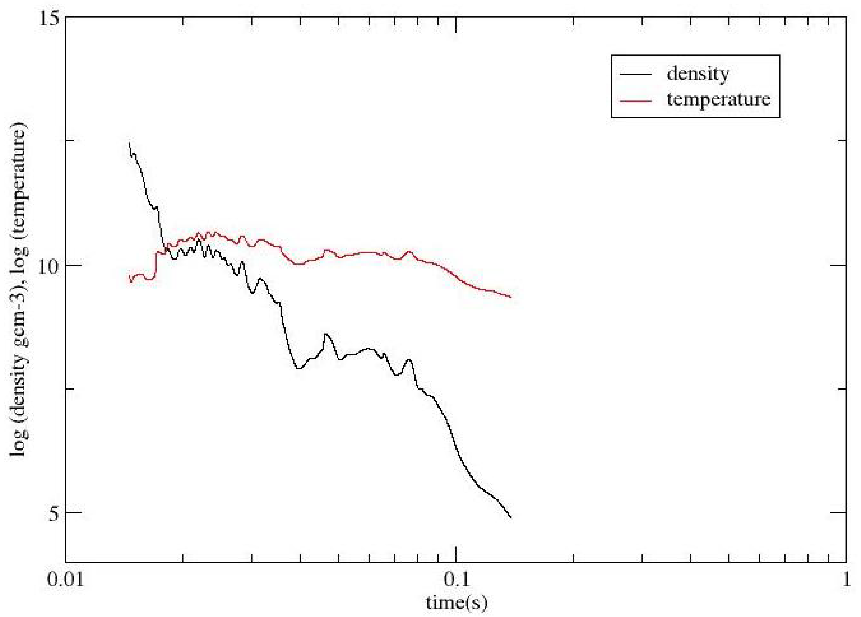
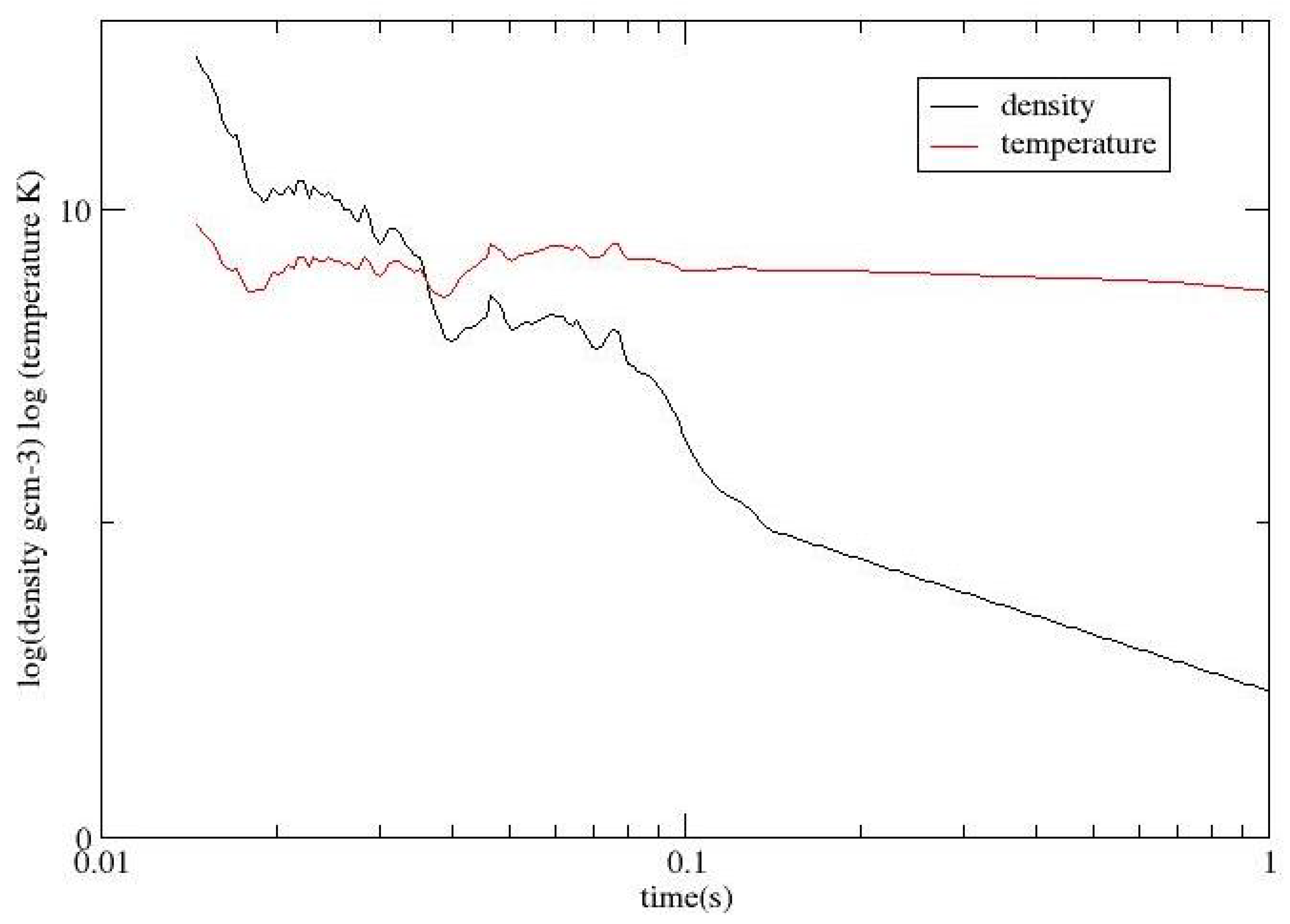
Figure 1 and
Figure 2 show the temperature and densities (without and with self-heating) of case16(Ye=8.07E-02). The case chosen as the neutron degeneracy has the biggest effects on it. We will present the effects in the Results section.
2.2. Degeneracy Factor and Neutron Fermi Energy
Next, we use a degeneracy factor to decide whether the neutrons in the ejecta of the merger are degenerate or not. The degeneracy factor is defined as the neutron chemical energy divided by the energy of the temperature:
where
is the chemical potential of the neutron,
k is Boltzmann’s constant, and
T is the temperature. We define the degeneracy factor larger than 1 is neutron degenerate.In the Results section, we will show that the neutrons are degenerates at the beginning as well as during the r-process. In reality,
(the neutron chemical potential) depends on the equation of state of the neutron star. For simplicity, we approximated the neutrons as a Fermi gas. We assume the neutron chemical potential is equal to the Fermi energy of a non-interacting Fermi gas which is
where
ℏ is Planck’s constant,
is the Fermi energy of the neutrons,
m is the mass of the neutron, and
is the number density.
2.3. SkyNet
The code SkyNet Lippuner and Roberts [
26] was used to perform the calculations of the nuclear reactions in the ejecta of a merger. For the beta decay rates, we used the Fuller and Fowler (FFNU) rates Fuller [
27], Langanke and Martinez-Pindo [
28]. For the theoretical partition function, we used the WINVN file [
29]. We included fission in the SkyNet Panov et al. [
30], Panov et al. [
31] but neutrino reactions were not included.
At the beginning of the merger, the neutron capture rates were so high that the time steps had to be made too small for the tracking. NSE was assumed. The Saha equations were used to calculate the NSE.
The Saha equation for an ideal Maxwell–Boltzmann gas is [
32]
The present paper studies the effects of neutron degeneracy on the r-process. Thus the Saha requires modification. The Saha equations using the neutron degeneracy corrections to a Fermi–Dirac distribution can be found in Lau [
33]. Here we repeat that derivation.
First, we can approximate the nuclei other than neutrons as a Maxwell–Boltzmann gas due to their small abundances. The typical highest abundances of the nuclei are around 1.0E-4 and the nuclei have larger atomic masses, typically on the order of 100 times that of the neutron. Thus it is valid to assume the nuclei other than the neutrons are a Maxwell–Boltzmann gas. For an ideal Maxwell–Boltzmann gas,
where
is the number density of nuclei
A,
is the number density of nuclei
,
J is the spin,
m is the mass,
is Boltzmann’s constant,
T is the temperature,
ℏ is Planck’s constant, and
is the chemical potential; while
We assume neutron capture and photodisintegration rates are at equilibrium of a single isotope here because the rates are much faster than the beta decay rates due to the high temperatures in such a merger. This is not a bad assumption. In equilibrium, the chemical potential is
The
can be written as follows:
Combining the above equations, the corrected Saha equation (directly using the neutron densities) is
Thus the correction factor is
f:
Thus, the simplest way to modify the original SkyNet code (which uses the typical Saha equations) is simply directly multiplying the formula in the NSE subroutine in the code by the correction factor f.
After NSE, the Skynet code calculates the nuclear reactions using the following formula:
where
is the abundance of isotope
i,
N is the number of isotopes,
is the rate of the one-body reaction,
are the rates of the two-body reactions,
are the rates of the three-body reactions,
is Avogadro’s number, and
is the density.
For the nuclear physics input, we implemented the JINA REACLIB from Cyburt et al. [
22] but with a correction factor for the neutron capture rates. We justified we only modified the neutron capture rates by the following arguments.
For reactions involving photons, we find for the overall reaction rate 0+1
+ 3
where
r is the net rate,
N is the number of isotopes,
is the photo-disintegration rate, and
is the two-body reactions. We assume the neutron capture and photo-disintegration rates are not too far away from equilibrium at high temperature and high densities when the degeneracy factor is larger than 1 (See
Figure 2 and 3). Thus,
r is roughly zero. Thus the distribution of nuclei can be represented by the following equations:
Thus, the distribution of nuclei are equivalent to the ratio of neutron capture rates to photodisintegration rates. Multiplying the correction factor to the neutron capture rates (or dividing the photodisintegration rate by the factor) can represent the change in the distribution of nuclei due to neutron degeneracy. This approximation in the Lau thesis [
33] got similar results in [
34] with exact rates [
35]. We believe that it is a good approximation.
2.4. Procedure
We first included the correction factor f in the NSE subroutine in SkyNet and picked out the abundances (other than those for neutrons) and directly multiplied the abundance equations in the NSE subroutine by the correction factor and then let the subroutine do the iterations. Thus, the iterations will find the neutron abundances and chemical potentials which fulfill the Saha equations. The NSE subroutine outputs the initial abundances in the merger.
For the initial conditions, we chose a density that is below and temperature higher than 1 GK but lower than 10 GK in order to fulfill the NSE condition. The smallest times which satisfy both conditions were chosen.
We also implemented the correction factor in the neutron capture rates inside the code. Since we want to study the distribution of the nuclei, only the ratio of the neutron capture rates to the photodisintegration rates is our interest. Either multiplying the neutron capture rates with the correction factor or dividing the photodisintegration rates with the same factor gives the same result. Thus, we picked out the neutron capture rates and multiplied them by the correction factor before they entered the matrix solver to calculate the abundances.
For a degeneracy factor smaller than 1, we stop multiplying by it within the code because the approximation only holds for high neutron degeneracy.
Finally, in order to see if our result are reliable, we studied all the situations with different values of mass deviation thresholds as well as to check the numerical convergence. We found that they have no observable effect on the results.
3. Results
3.1. Neutron Degeneracy in the R-Process
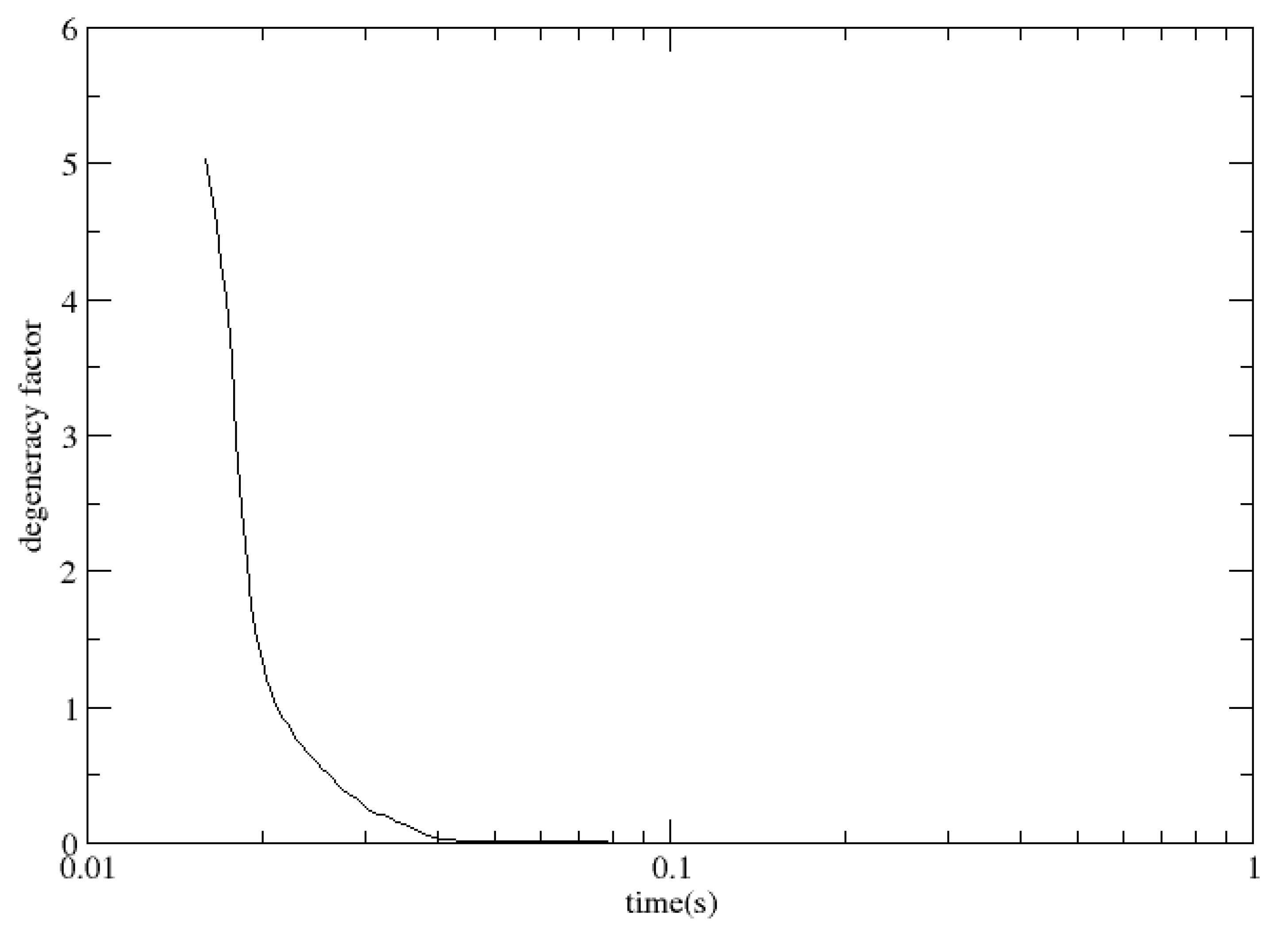
First, we show that neutrons may be degenerate during the r-process in NS-BH mergers. In general, the neutrons are degenerate all the time before the degeneracy factor reaches 1.
Figure 3 shows a typical case (case16) of the degeneracy factor versus time.
Table 1 shows the time, temperature, density, and electron abundance at the start of the r-process for each case. We defined the beginning of the r-process as the point of the start of the building up of the nuclei in the second peak of the solar abundances.
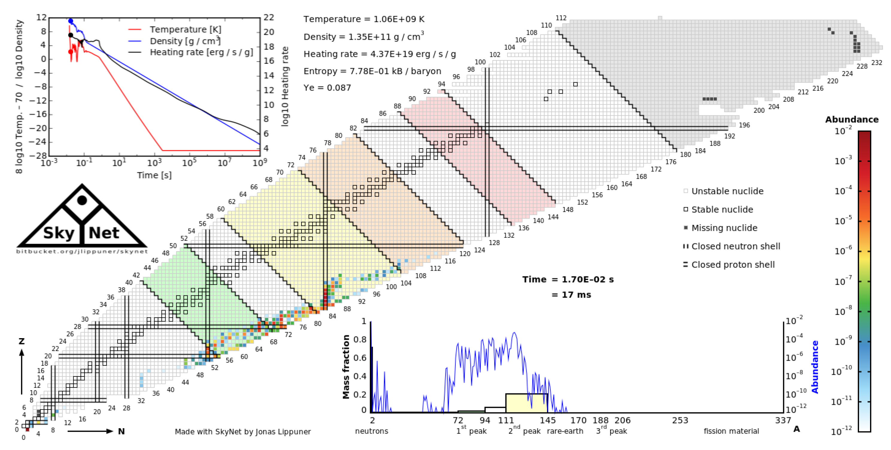
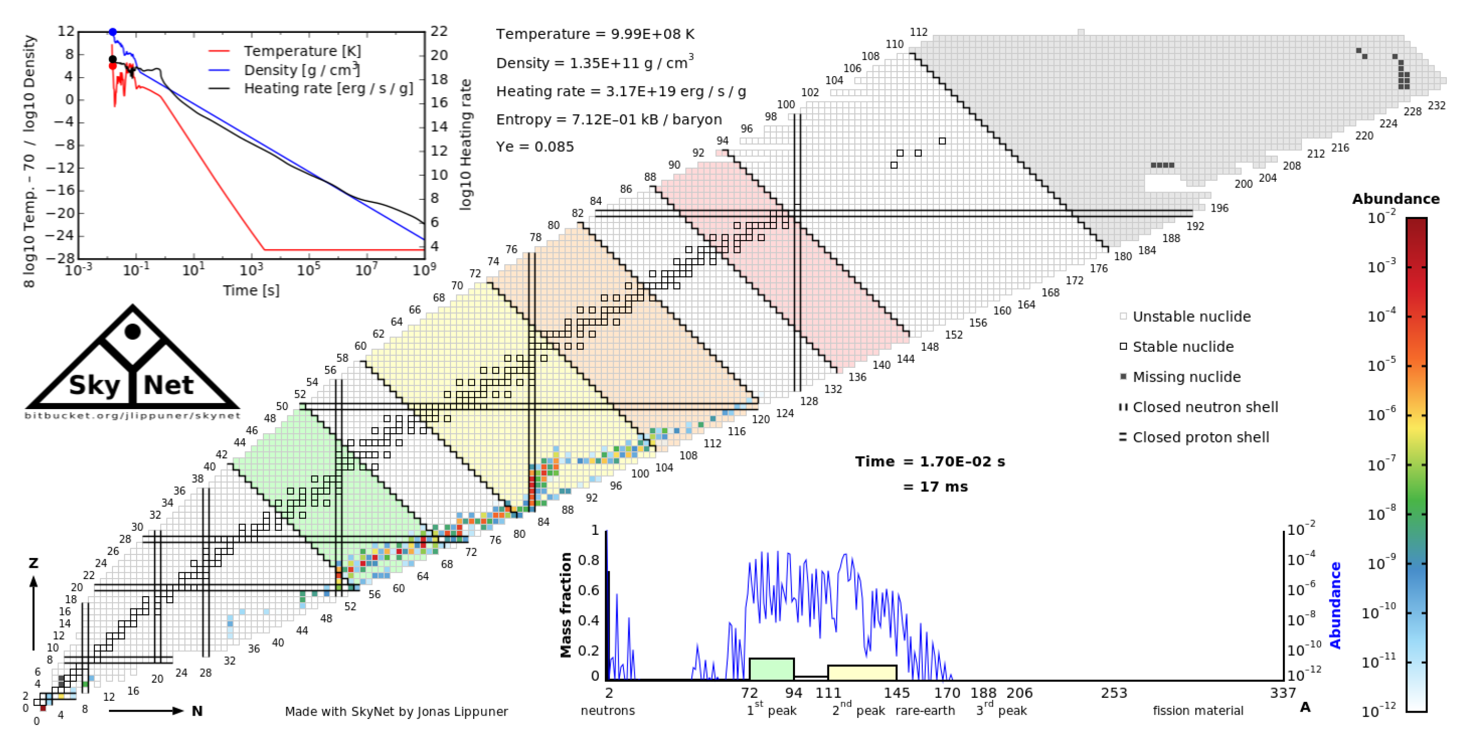
Figure 4.
Abundance plot when the r-process starts (without correction)
Figure 4.
Abundance plot when the r-process starts (without correction)
Table 2 shows the time, temperature, densities and electron abundances when the degeneracy factor reaches 1. We can see the r-process started before the degeneracy factor reached 1 for all cases expect case 5. This shows that neutrons may be degenerate during the r-process.
3.2. Heating Effects on Temperature Changes
After running 20 trajectories with and without neutron degeneracy correction, we discovered that such a correction can have big effects on the heating in the r-process and hence the temperatures in some cases.
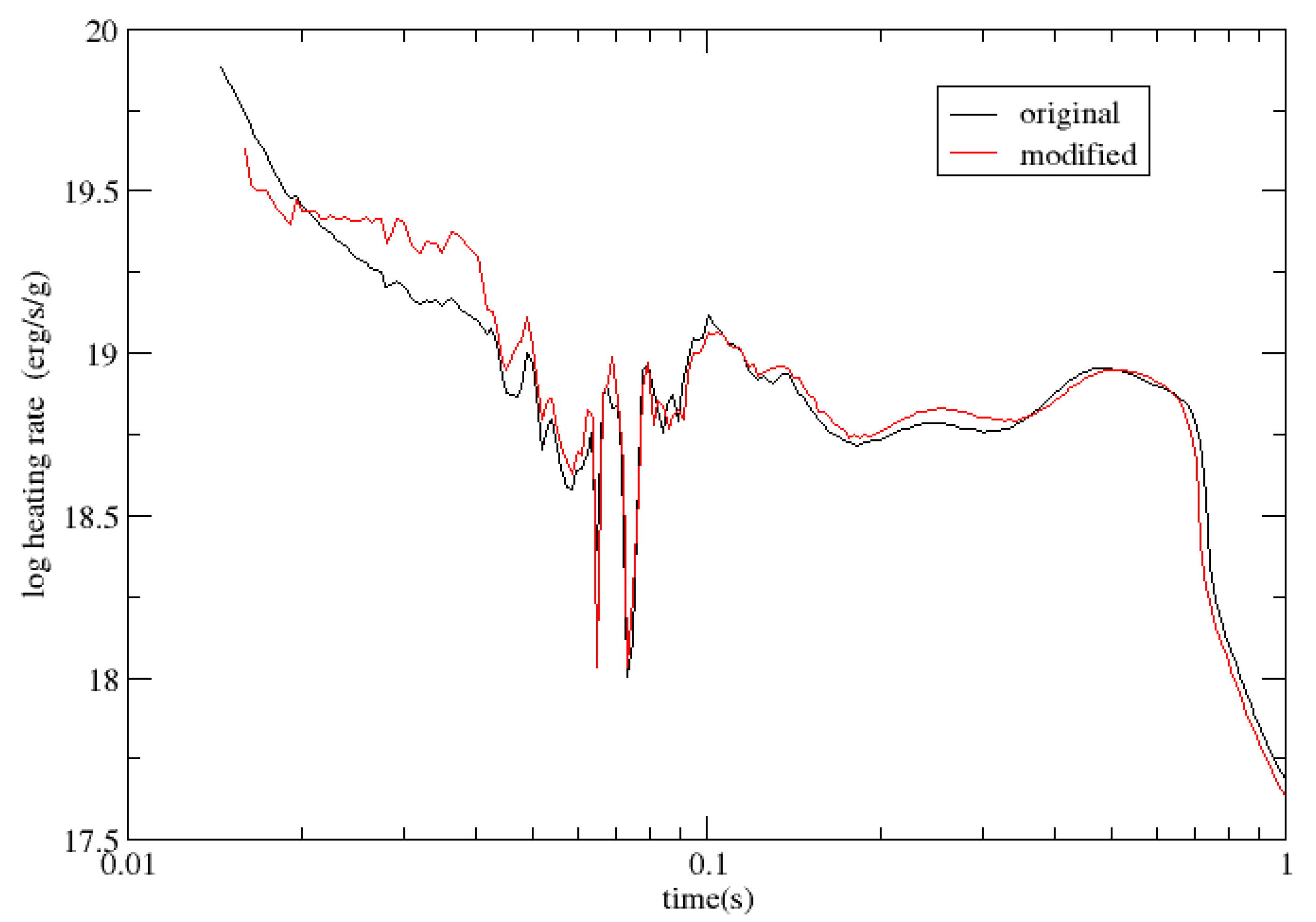
Figure 5 shows the heating rates with and without neutron degeneracy for case 16.
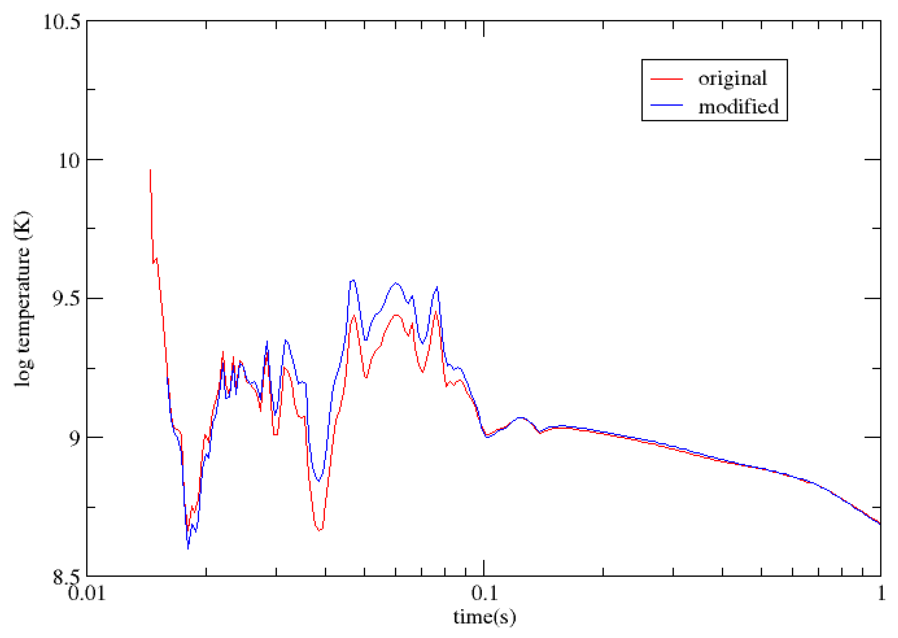
Figure 6 shows the corresponding situations for the temperatures.
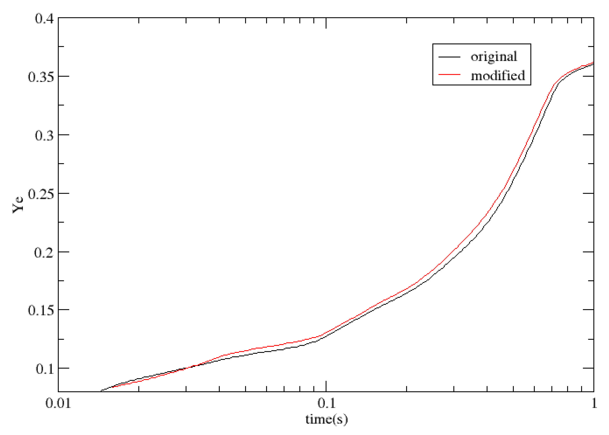
Figure 7 shows the electron abundances of case16 with time.
From
Figure 5,
Figure 6, and
Figure 7, we can see the heating rates, temperatures, and electron abundances versus time. At the beginning, from
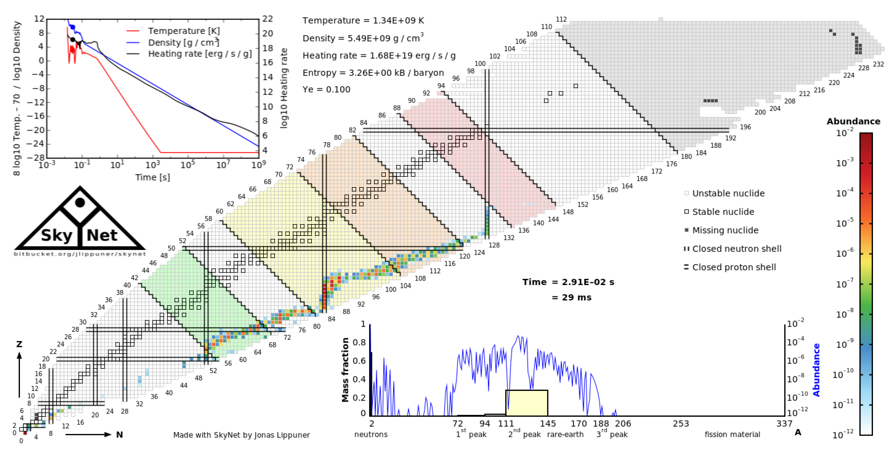
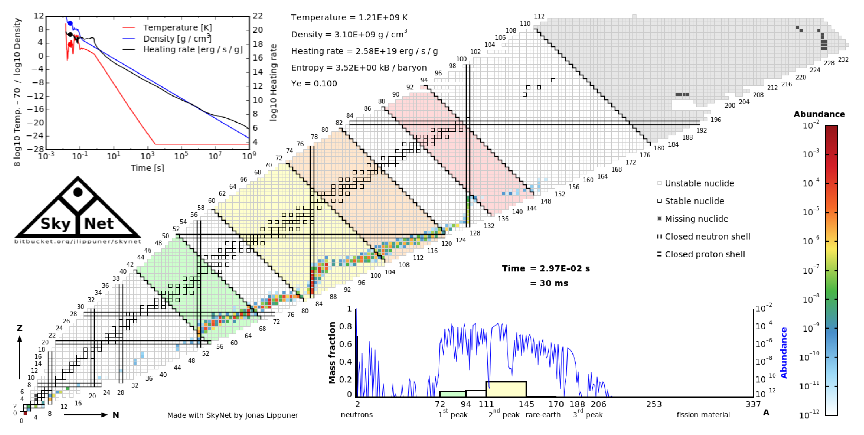
Figure 8 and
Figure 9, we can see degenerate neutron capture rates shift more nuclei to the neutron-rich sides (see Equation 1), as well as that the value of degenerate Ye is smaller than that for the non-degenerate Ye, leading a decrease in energy due to the negative
of the neutron capture rates for neutron-rich nuclei. Later on (after 22 ms), due to the higher mass of the nuclei produced,the beta decay neutron emissions rates for high masses are much higher than those for the low masses, the heating rates increase and hence lead to increases in temperature (one can see that for Ye it is higher in the presence of degeneracy than in the absence of degeneracy). One of the remarkable things is that there are also differences in the heat produced after the degeneracy effect is gone (
s). After 0.1 s, the effects due to neutron degeneracy are completely gone.
Figure 8,
Figure 9 and
Figure 10 show the abundance plots, which are the distribution of the nuclei (with and without neutron degeneracy correction) for different times. The abundance plot without neutron degeneracy correction at 17 ms was shown in
Figure 4 in the previous subsection.
3.3. Final Abundances
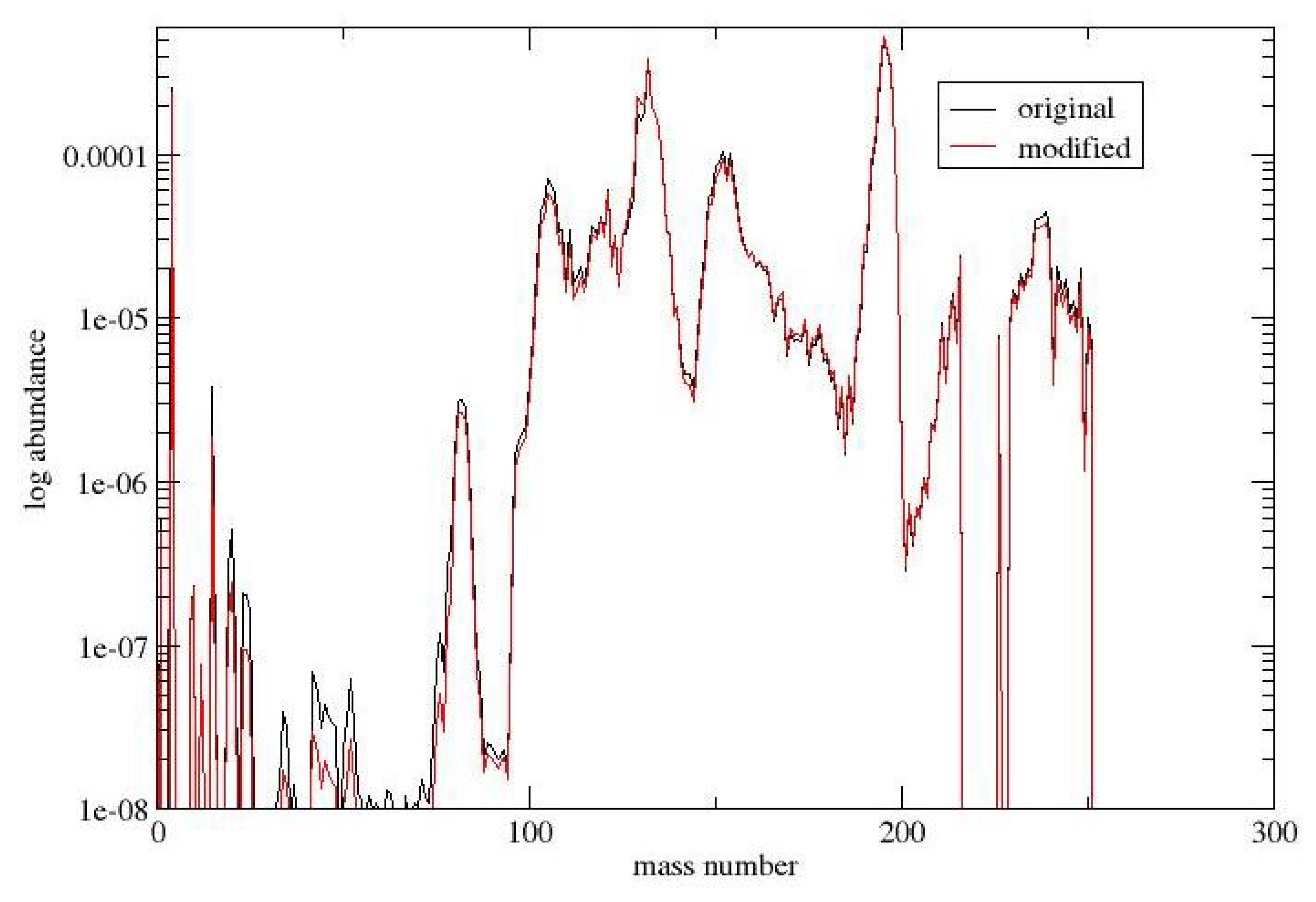
Comparing the final abundances with and without neutron degeneracy, we find that there is not much difference. This is expected, as the degenerate neutron capture rates happen in the early stages of the r-process and the effects are washed out by later nuclear reactions and hence have little effect on the final abundances.
Figure 7 shows one of the cases (Case 16).
Figure 11.
Final abundances in Case 16
Figure 11.
Final abundances in Case 16
4. Discussion
The trajectories of a NS-BH mergers were used to study the effects on the production of heavy elements in the r-process in Rosswog et al. [
12], Rosswog et al. [
14]. They examined different trajectories and concluded that the final abundances produced are kind of consistent with the solar abundances. We reach the same conclusion as well. The final abundances can reproduce the features of the solar abundances.
From the result section, we can see that the consideration of neutron degeneracy mostly increase the temperatures of the system, thus leading in brighter light curves. The detailed impacts due to the degeneracy on the light curves can be further investigated.
The beta delayed neutron emission rates may also decrease as the neutron emissions may be blocked due to the high Fermi energy of the neutron. These reactions may lead to further changes in the final abundance and the heat generation of the the r-process. However, a set of consistent rates with a neutron degeneracy correction are not presently available. Thus, we leave it to be done in future projects.
Actually, the neutron chemical potential should be higher than the Fermi energy, as the neutrons should have interactions. The effects of the light curves actually may even be stronger.
Furthermore, neutron degeneracy may also need to be taken into account in the r-processes in other scenarios, such as NS-NS mergers and hypernoave, possibly revising the final abundances and heat generation.
5. Conclusions
In this paper, we first showed that neutrons can be degenerate in the ejecta at the beginning as well as during the NS-BH merger (in an r-process). This neutron degeneracy has effects on the distribution of the nuclei and therefore the heat generation and hence the temperature of such a merger. This can result in a brighter light curve. However, this has little effect on the final abundances. Neutron degeneracy can also affect the nuclear reactions in the r-process such as beta-delayed neutron emissions during the r-process. This may also further affect the final abundances as well as the heat generation in the r-process. Moreover, neutron star mergers and hypernovae may also have neutron degeneracy effects. This issue should be further studied.
Funding
This research received no external funding.
Data Availability Statement
The raw data supporting the conclusions of this article will be made available by the authors on request.
Acknowledgments
The author wants to thank Hendrik Schatz and Otto Tang for discussions of the project.
Conflicts of Interest
The authors declare no conflicts of interest.The funders had no role in the design of the study; in the collection, analyses, or interpretation of data; in the writing of the manuscript; or in the decision to publish the results.
References
- Burbidge, E.M. ; others. Rev of Modern Phy 1957, 29, 547–650. [Google Scholar] [CrossRef]
- Arcavi, I. ; others. Nat. 2017, 551, 64–66. [Google Scholar] [CrossRef]
- Pian, E. ; others. Nat. 2017, 551, 67–70. [Google Scholar] [CrossRef] [PubMed]
- Abbott, B.P. ; others. Phys. Rev. Lett. 2017, 119. [Google Scholar]
- Smartt, S.J. ; others. Nat. 2017, 551, 75–79. [Google Scholar] [CrossRef] [PubMed]
- Valenti, S. ; others. ApJL 2017, 848, L24. [Google Scholar] [CrossRef]
- Cowperthwaite, P.S. ; others. ApJL 2017, 848, L17. [Google Scholar] [CrossRef]
- Abbott, B.P. ; others. Phys. Review X 2021, 11. [Google Scholar]
- Broekgaarden, F. ; others. ApJL 2017, 920, 13. [Google Scholar] [CrossRef]
- Surman, R. ; others. ApJ 2008, 679, L117. [Google Scholar] [CrossRef]
- Goriley, S. ; others. ApJL 2011, 738, L32. [Google Scholar]
- Rosswog, S. ; others. MNRAS 2013, 430, 2585–2604. [Google Scholar] [CrossRef]
- Wanajo, S. ; others. ApJL 2014, 789, L39. [Google Scholar] [CrossRef]
- Rosswog, S. ; others. CQG 2017, 34. [Google Scholar]
- Foucart, F. Front
. Astron. Space Sci. 2020, 7. [Google Scholar]
- Siegel, D. Nature Review Physics 2022, 4, 306–318.
- Barbieri, C. ; others. A & A 2019, 625. [Google Scholar]
- Ackley, K. ; others. A & A 2020, 643. [Google Scholar]
- Barbieri, C. ; others. The European Physical Journal A 2020, 56. [Google Scholar]
- Anand, S. ; others. Nature Astronomy 2021, 5, 46–53. [Google Scholar] [CrossRef]
- Freiburghaus, C. ; others. ApJ 1999, 525, L121. [Google Scholar] [CrossRef]
- Cyburt, R.H. ; others. ApJS 2010, 189, 240. [Google Scholar] [CrossRef]
- Cyburt, R.H. ; others. ApJ 2016, 830, 55. [Google Scholar] [CrossRef]
- Piran, T. ; others. MNRAS 2013, 430. [Google Scholar]
- Korobkin, O. ; others. MNRAS 2012, 426. [Google Scholar]
- Lippuner, J.; Roberts, L.R. ApJS 2017, 233, 18.
- Fuller, G.M. ApJS 1982, 48, 279–320.
- Langanke, K.; Martinez-Pindo, G. Atomic Data and Nuclear Data Tables 2001, 79.
- Rauscher, T. ApJS 2003, 233, 403.
- Panov, I. ; others. AstL 1995, 21. [Google Scholar]
- Panov, I. ; others. AstL 2001, 27. [Google Scholar]
- Illiadis, C. Nuclear Physics of Stars, Wiely 2007.
- Lau, K.Y. PHD thesis, Michiagn State University 2012.
- Lau, R. ; others. ApJ 2018, 859. [Google Scholar]
- Shternin, R.o. Phy Rev C 2012, 86.
|
Disclaimer/Publisher’s Note: The statements, opinions and data contained in all publications are solely those of the individual author(s) and contributor(s) and not of MDPI and/or the editor(s). MDPI and/or the editor(s) disclaim responsibility for any injury to people or property resulting from any ideas, methods, instructions or products referred to in the content. |
© 2024 by the authors. Licensee MDPI, Basel, Switzerland. This article is an open access article distributed under the terms and conditions of the Creative Commons Attribution (CC BY) license (http://creativecommons.org/licenses/by/4.0/).
