Modelling Livestock Weights in a Marketplace Using Computer Vision Technologies

Livestock marketplaces consist of infrastructure and rules through which information is exchanged and transactions are completed. Livestock trading incurs significant transaction costs, beyond just commission fees paid to marketplace owners (e.g., se-lecting, loading and transporting animals). In addition, animals being transported, held and transacted in a market setting increases the likelihood of injury or disease. The Covid-19 pandemic contributed to large-scale changes across typically physical marketplaces as stay-at-home orders and travel restrictions were invoked. Livestock marketplaces pivoted online rapidly, facilitated by the deployment of video feeds, al-lowing buyers to view/purchase animals via mobile phone. This shift offered the promise of mitigating many of the transaction costs associated with a fully physical marketplace. This study evaluated how computer vision (CV) approaches can con-tribute to the evolution of livestock marketplaces. It used livestock video data for 240 cattle (bulls) weighing 320-740 Kg from 16 different breeds to elicit additional trade-relevant data (livestock weight) and can be considered as an intermediary step to better understand how video data can be used to further digitalize livestock trade, price formation and transaction completion via technology solutions. The dataset comes from three sales held on different dates in a single mart location, which allows a consistent camera setup throughout. CV technologies were employed to solve the problem of cattle weight estimation and a distinctive achievement lies in curating a dataset cap-turing cattle in motion within the context of a cattle auction thereby injecting realism and complexity into the CV weight estimation task. Employing advanced object detection algorithms, the study created an intricate data pipeline to generate an appropriate modelling dataset and devised new multi-channel architectures for deeper analysis of diverse image inputs. The significance of sizable datasets and the challenge of man-aging inherent input variability for accurate CV regression is highlighted. Top-down view predictions demonstrate comparatively better performance, although failing to achieve benchmark precision. Challenges arise from camera angle variations, roaming behaviors, and breed diversity. Likewise, side-view predictions face challenges due to increased variability and lack of standardization. Despite this, these predictions offer insights into the value of incorporating Region of Interest (ROI) coordinates and data augmentation for enhanced performance. The study concludes with a multi-input ar-chitecture combining top-down and side-view predictions, demonstrating moderate success highlighting potential synergy between both perspectives. The central con-clusion resonates strongly – using standardized and multi-view images encompassing controlled movement and consistent poses could bolster accurate CV weight estima-tion.

Keywords:

Subject: Computer Science and Mathematics - Computer Vision and Graphics

1. Introduction

Roth (2018) notes that ‘marketplaces…consist of infrastructure, rules, and customs through which information is exchanged and transactions are made’. Computer vision (CV) applications have been shown to support animal health monitoring (Fernández-Carrión et al., 2020) and population dynamics (Weinstein, 2018), for example. This paper explored the application of CV to these novel environments as a precursor to evaluating the potential of completing agricultural transactions in new ways and thus contributing to the future design of livestock marketplaces. While the concept of predicting animal weight from video is not novel, this study is different due to the unique characteristics of its dataset. Unlike traditional datasets, which often feature controlled environments with standardized conditions, this dataset includes footage where animals roam freely within the video frame. This lack of control introduces significant variability and noise, such as the presence of human shepherds and background activity from bidders, making the problem substantially more challenging. The contribution of this research to the field is the demonstration of the practical challenges and computational demands associated with processing non-standardized, real-world video data. The findings emphasize the advantages of using standardized image inputs, the necessity for extensive datasets, and the requirement for substantial computational power to achieve accurate predictions.

It is well established that bodyweight (BW) and BW changes in livestock are powerful predictors (Cominotte et al., 2020) that can inform crucial decisions in farm management (Qiao et al., 2020). These metrics play a pivotal role in successful genetic selection (Rezende et al.,2022), optimizing fertility rates (Domecq et al., 1997; Berry et al., 2002; Wathes et al., 2007), assessing animal health status (Roche et al., 2013), optimizing overall productivity (for example, milk yields in dairy cattle) (Mushtaq et al., 2012), and identifying the best time to market animals (Gjergji et al., 2020). BW dramatically influences the market or factory price of an animal, i.e., the monetary value of livestock can be roughly defined as weight of meat × price/kg (Pethick et al., 2021). Moreover, weight measurements find diverse applications, such as determining the correct dosage of therapeutics, optimizing feed amounts, and identifying the ideal weaning time (Lesosky et al., 2012).

Despite the undeniable significance of weight-related data in livestock management, this metric remains vastly underutilized. However, adopting a technical solution to solve this is not due to the agriculture industry’s slow adoption of innovative technologies; rather, it stems from the complexity of addressing this challenge. In recent years, the cattle industry has witnessed a revolutionary transformation with the introduction of new technologies. For instance, robots have been employed to assist farmers, contributing to increased efficiency and productivity (Nabokov et al., 2020). Moreover, cutting-edge AI applications have also made inroads into the cattle industry. These advances demonstrate the industry’s readiness to embrace novel technologies to improve livestock management practices.

The difficulties of fully utilizing weight metrics reside in the significant constraints associated with the current weighing technologies, which tend to lack accuracy and/or feasibility. Currently, the most basic method to obtain cattle’s BW is simply using weighing scales. However, this seemingly straightforward approach poses several challenges beyond surface-level considerations. Industrial scales designed for animals can be prohibitively costly for small/medium-sized farmers, making it unfeasible for them to adopt this technology. Moreover, obtaining weight measurements using traditional scales may require significant manpower, which could add to the operational burden on farmers. Additionally, physically weighing the animals can cause stress to the livestock, affecting their well-being (Cominotte et al., 2020; Grandin and Shivley, 2016). Given these limitations, it becomes evident that there is a clear requirement for a more innovative and accessible solution for weight estimation in cattle.

To unlock the untapped potential of this valuable metric, efforts should be directed towards developing user-friendly and accessible solutions to accurately predict and monitor the weight of livestock. By democratizing access to such solutions and, in this case, optimizing the use of BW and BW changes in livestock management, all farmers, regardless of their scale of operation, can benefit from informed decision-making and enhanced productivity.

An exemplary case is the Irish company Cainthus, which has developed a cattle facial recognition solution to monitor the health and well-being of livestock. The practicality and potential success of employing CV techniques are at the heart of the current study and it encompasses the end-to-end pipeline of data acquisition, video/frame preprocessing, model development, and evaluation. With a systematic examination of each step and an iterative refinement approach, the goal is to determine the feasibility of a CV solution capable of reliably estimating the BW of cattle, a crucial parameter in livestock management.

By leveraging advanced image processing and deep learning algorithms (see, for example, Oliveira et al. (2020)), this study seeks to determine the extent to which CV can provide dependable weight predictions, considering a diverse set of breeds and weight distribution present in the Irish livestock industry. It also seeks to obtain precise body weight predictions for cattle captured in motion through video input. Furthermore, it explores the challenges posed by moving animals and “noisy” frames, aiming to ascertain whether CV methods, such as object detection and convolutional neural networks, can overcome these obstacles and yield reliable weight estimates. Finally, the study also explores the viability of developing a user-friendly phone application that harnesses CV algorithms. The theoretical application’s purpose is to empower users, including farmers and livestock professionals, to capture videos of cattle and receive reasonable weight estimates.

The following section reviews the literature on BW estimation of livestock and provides a comprehensive overview of the methods and technologies used to predict and monitor the BW of livestock, offering insights into the current state-of-the-art methods in this field. The methodology employed in the study is then described including the evaluation methods and the CV techniques used. The results are then presented followed by a discussion.

1.1. Livestock Bodyweight Estimation

Research on this topic can be seen as early as the 1930s. Brody et al. (1937) argue that body weight in dairy cattle can be estimated using the relationship between body weight and chest girth. This relationship was very simple as it required a single measurement that could be gathered using a tape measure. Although this method could not be expected to achieve exceptionally accurate results, they were indeed “close enough for practical weight estimation” (Brody et al., 1937). This weight estimation method can be classed as a ’traditional’ approach.

Wang et al. (2021) define the iterations of innovation in BW estimation of livestock as ‘traditional’ and CV approaches. The ‘traditional’ methods involve manually collecting morphometric measurements coupled with regression-type formulas. Although Brody et al. (1937) used the single feature/measurement of chest girth, there is a catalogue of literature using additional measures such as hip height, hip width, wither height, and body length, i.e., (Heinrichs et al., 1992; Enevoldsen and Kristensen, 1997; Ozkaya and Bozkurt, 2009). Throughout the tenure of these traditional approaches, several formulations were derived. Wangchuk et al. (2018) reviewed several of these ’traditional’ approaches on a sample of two different cattle breeds and found that Schaeffer’s formula performed the best with an average deviation from true weight of between 4.70 – 4.84 %. The Schaeffer formula is: W=(LxG²)/300 where W is body weight in lbs, L is the length of the animal from the point of shoulder to pin bone in inches, and G is the chest girth of the animal in inches (Wangchuk et al., 2018).

Although the level of accuracy achieved can vary significantly from study to study due to variation in breeds/animals and estimation methods used, for example, the literature suggests that traditional approaches achieve relatively good estimates (Wangchuk et al., 2018). Moreover, to derive such an estimate, the only requirement is to have a tape measure. As a result, these ‘traditional’ approaches still remain as the most widely used methods today. Similar to the limitations of commercial-grade weighing scales mentioned earlier, these methods also have their drawbacks, i.e., they suffer from the same labor-intensive and animal well-being issues but often result in unreliable estimates (Brandl and Jørgensen, 1996). Consequently, there is a growing effort to develop more accurate and less laborious techniques by leveraging cutting-edge technologies. Wang et al. (2021) introduce the concept of CV (use of images to estimate weight) approaches as the next stage of development.

1.2. Computer Vision Methods

The initial approaches that utilized digital images was limited to feature extraction. For example, Ozkaya (2013) derives the features of body length, wither height, chest depth, hip height, and hip width using images taken from a calibrated digital camera using photogrammetry. Feature selection was then conducted manually, and predictions were made using a traditional regression model. Although this method could achieve an R² value of up to 0.91 (Ozkaya, 2013), it was only a short time before the traditional regression models were replaced by the more complex machine learning models (Tasdemir and Ozkan, 2019), using a similar method as outlined by Ozkaya (2013), swapped out the regression model for an artificial neural network (ANN) and concluded that ANNs could be used in live weight prediction. Although a comprehensive comparison between both studies is not as straightforward as looking at the best R² value achieved, the literature suggests that (in general) given adequate data, the more complex machine learning models outperform the traditional regression models (Sathe and Venitz, 2003) and this result is not surprising. It is important to note that studies such as these tend to paint an overly optimistic picture. This occurs because the conditions are optimized (lighting, hardware, etc.), sample sizes are small, and although the testing set is unseen, it originates from the same herd, is taken at the same time, and has the same background (and thus noise) (Meer et al., 1991). Nevertheless, results such as these are very encouraging and provide hope that this technology can become standard in farmyards across the globe. Although using machine learning models for this use is a relatively new approach, Wang et al. (2021) define the most recent/current state-of-the-art approaches as the CV and Deep Learning approach.

The CV and deep learning approach “represents a first step toward the full automation of the BW prediction process using digital images” (Wang et al., 2021). The aforementioned CV approaches require at least 2 steps: 1) feature extraction, and 2) prediction. On the other hand, the deep learning approach typically includes image selection, feature extraction, and feature selection in a single step as part of a deep learning architecture, i.e., Gjergji et al. (2020).

It is important to note that this literature, while informative, is relatively limited and can be further subdivided based on the availability of hardware resources, e.g., the type of imaging equipment used. This study will focus on a subset that utilizes video data captured from basic cameras as imaging equipment. However, it is essential to acknowledge that other advanced imaging technologies, such as 3D images and RGBD (Red, Green, Blue, Depth) cameras, exist and have been explored with promising results. This has been demonstrated by Hansen et al. (2012) achieving an error rate of just 6.1 % using 3D imaging on a testing set of 185 cows.

Despite the potential of advanced imaging techniques, this study aims to expand the literature in a way that is feasible and accessible for small to medium-sized farmers, where more expensive hardware may be prohibitive. By focusing on basic camera setups, this study seeks to provide practical and cost-effective solutions to benefit a broader range of potential consumers in the agricultural sector.

Gjergji et al. (2020) explore the application of deep learning methods to predict beef cattle’s BW. The camera was set up with a top-down view directly above where the animal drinks water from a trough. Additionally, the animals must step on a weighing scale to access the water. As a result, whenever the animals go for water, their weight is recorded, and images are captured simultaneously. Furthermore, an RFID antenna is used to identify when an animal is positioned on the platform (scales). Several CV methods are then deployed; included CNNs (convolutional neural networks), RNNs (recurrent neural networks), as well as a CNN/RNN combination model, while also incorporating some models that leveraged transfer learning. The RNN/CNN combination architecture emerged as the most accurate. This model used the pre-trained EfficientNetB1 CNN architecture with ImageNet weights and employed L1 Loss/MAE (mean absolute error) loss. As a result, the model achieved a MAE of 23.19 Kg on the hold-out test set. This is a significant improvement on the previous top CV, linear regression models which reached an error of 38.46 kg (Weber et al., 2020). However, the authors acknowledged that this approach exhibited limitations, particularly in dealing with noise, such as instances when stray cattle entered the frame. They noted the need for future work to address this issue and improve the model’s robustness.

2. Material and Methods

The dataset in this research consists of various cattle breeds captured in motion with a comprehensive weight distribution across the training set, presenting unique challenges in accurately estimating weights from video data. Due to the “noisy” nature of the video input (i.e., cattle in motion, human market participants, etc.), a crucial step is to obtain localized information about the cattle’s appearance and behavior, facilitating more precise weight estimation. Object detection algorithms were explored and used to create a training set for the final prediction algorithms. The predictive models utilized were CNN-based approaches, such that customized architectures were designed and tailored specifically for cattle weight prediction using the extracted frames. CNNs have demonstrated remarkable success in various CV tasks (Chougule et al., 2018) and we explored their potential in accurately predicting cattle weights.

2.1. Dataset

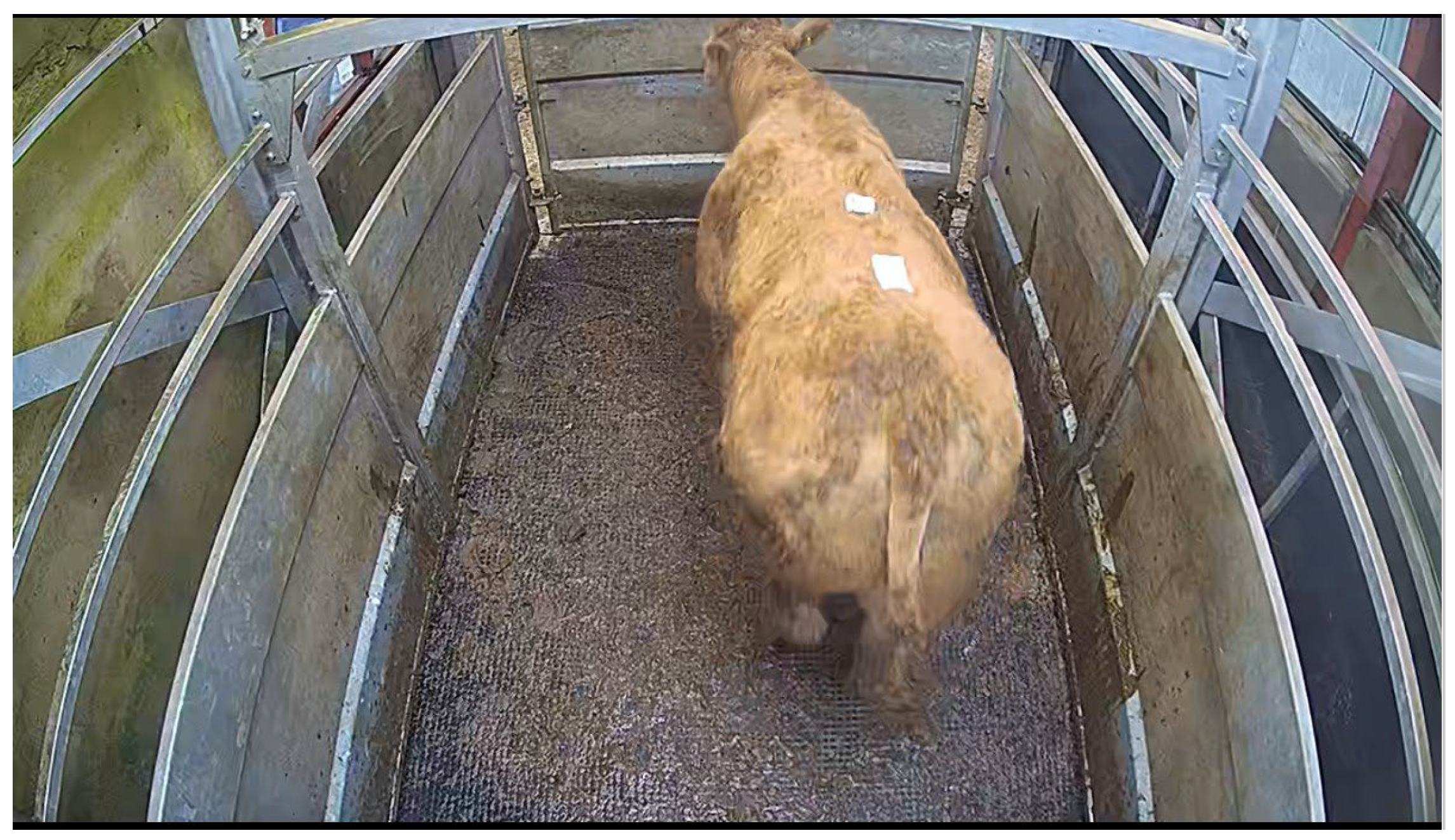
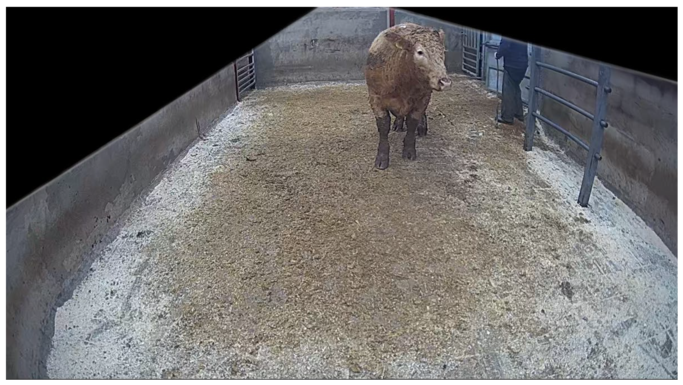
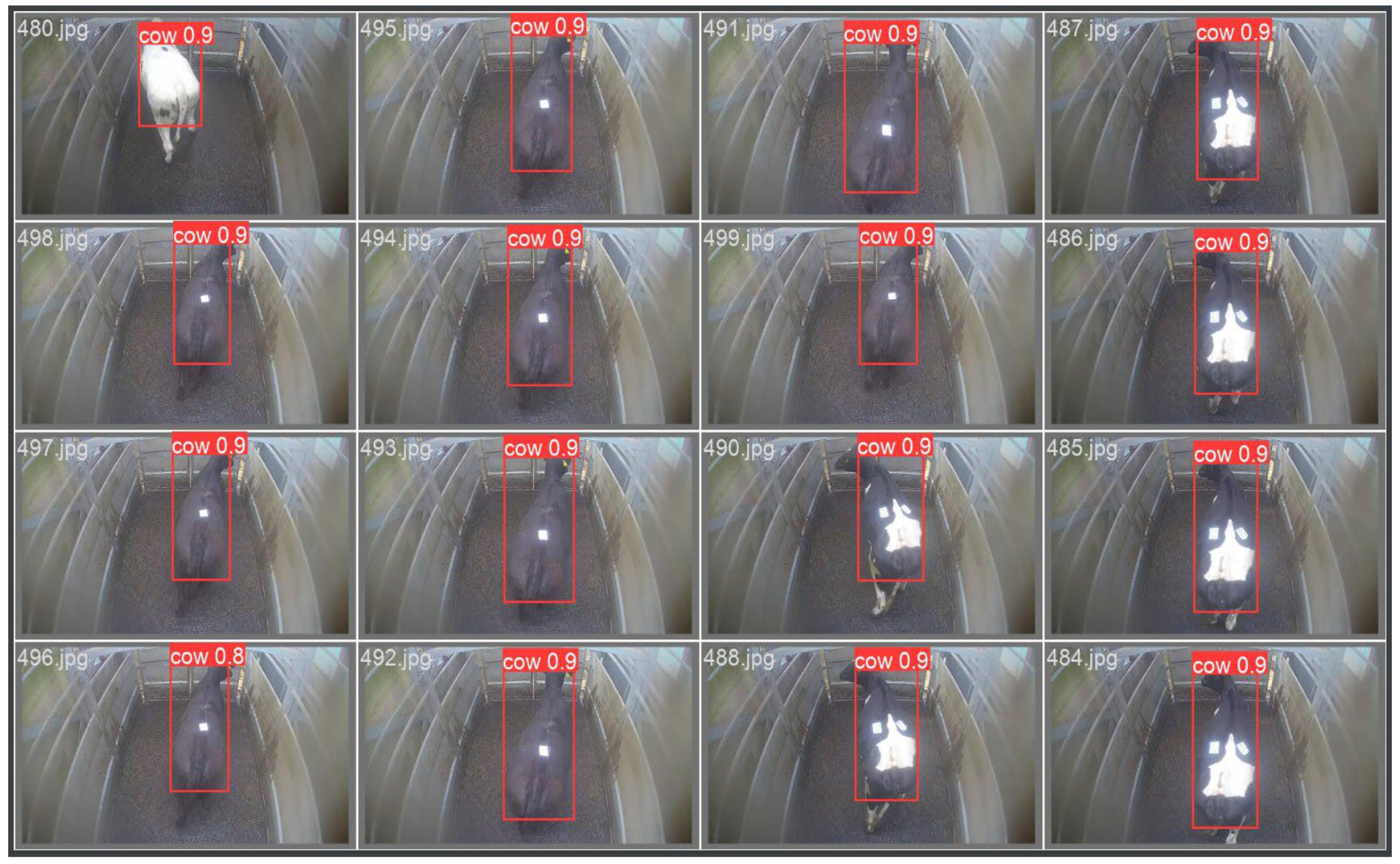
The data used in the current study is provided by Marteye, an Irish agricultural technology company. Video for 240 cattle is analyzed in the current study. These animals are all bulls (male), have weights ranging from 320-740 Kg and include 16 different breeds (e.g., Angus, Limousin, Charolais, Freisian, Hereford, Simmental, Belgian Blue and Holstein). There is a variable amount of footage. The dataset comes from three different sales held on different dates/times (November 2022), but the entire dataset is a single mart location, and therefore, the camera setup is consistent throughout. Note that weight is captured to the nearest 10 kg, and the camera resolution is 1280x720 pixels. There are two views available per animal, 1) top-down view (Figure 1) obtained as the animal enters the weighbridge and 2) side view (Figure 2) obtained when the animal enters the ring as the bidding begins.

The bull first enters the weighbridge (top-down) before entering the bidding ring (side-view). In this example, 40 seconds of footage were obtained in the top-down and 24 seconds in the side view. The input data to the weight prediction models will be frames of individual cattle. For a CV model to work well given a problem of this complexity, a significant amount of data is required (Vapnik et al., 1994). Therefore, given this paper’s dataset of 240 cattle, multiple frames must be extracted per animal.

To avoid training on data points (frames) that are a near identical match to those seen in the validation or testing sets, each dataset is separated via unique cattle, i.e., 70% of the cattle will be used to train, with 15% being used for both validation and testing sets.

2.2. Object Detection

To predict cattle weight from videos featuring animals in motion, object detection addresses the challenges posed by “noisy” frames and moving animals. Furthermore, object detection allows for implementing models that do not require analyzing the entire frame, which is crucial from both practical and computational perspectives. By focusing solely on the identified cattle, the weight prediction model can analyze relevant features without distractions, thereby improving accuracy. Another significant benefit of object detection in this context is its potential for better generalization to new environments, enhancing its real-world applicability.

YOLO (You Only Look Once) is an object detection algorithm that works by dividing the input image or video into a grid and predicting bounding boxes and class probabilities within each grid cell. Redmon et al. (2016) simplified the YOLO methodology as follows: “Processing images with YOLO is simple and straightforward. Our system (1) resizes the input image to 448 × 448, (2) runs a single convolutional network on the image, and (3) thresholds the resulting detections by the model’s confidence” (see Figure 3).

The single-pass architecture of YOLO is important as a relatively large quantity of video must be processed. YOLO has been shown to be accurate in object detection tasks (Redmon et al., 2016) and it has the ability to use both customizations via feeding the algorithm with hand-made annotated images or simply using extensively tested pre-trained models (Jiang et al., 2022). It is also relatively simple to implement and has excellent community support.

2.3. Deep Learning Model Architectures

Deep learning is a subset of machine learning that involves training artificial neural networks to learn from data. “Deep” refers to multiple hidden layers in these networks, allowing them to learn complex patterns and hierarchical representations from raw data (LeCun, 2015). The requirement for “deep” models in cattle weight prediction is twofold. Firstly, the complexity associated with this problem demands relatively complex models to learn the patterns and relationships from video data. Secondly, the nature of the image input itself contributes to the need for deep models. When using images as inputs for a learning model, the data size becomes relatively large, even when downsized to a standard format like (224, 224, 3) pixel dimensions, i.e., a square image of dimension 224x224 with three channels for RGB (Red, Green, Blue).

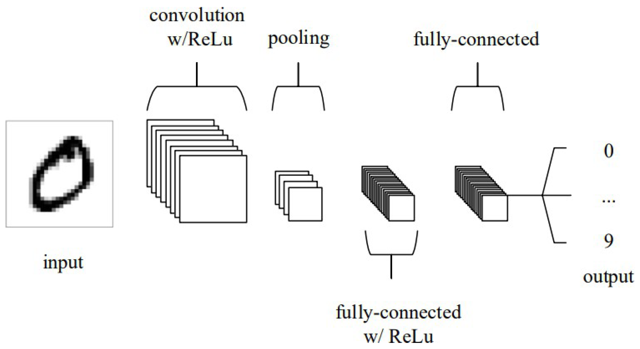
The deep learning models explored deploy CNN and RNN architectures. CNNs and RNNs represent a natural evolution from the original concept of Artificial Neural Networks (ANNs). Drawing on the basic CNN architecture set out by Vedaldi and Lenc (2015), CNN functionality can be split into four key areas in the current application. Firstly, the input layer will hold the pixel values of the input image. This paper will feed images of cattle (defined by pixel values) where 1 (greyscale) or 3 (RGB) channels per input will be considered. Second, the convolutional layers detect various features in an input image. This is achieved by using small filters (also called kernels) that slide over the input image to detect patterns such as edges, corners, and textures. The user must pre-define the number of convolutional layers and the number of filters per layer (see Figure 4 below).

Thirdly, the pooling layer will then perform downsampling. When working with CNNs, the parameter count gets very large quickly. Downsampling along the spatial dimensional helps reduce the number of parameters to retain as much important information as possible. Finally, the fully connected layers will then perform the same duties found in standard ANNs. In the above example, a classification problem is considered. This paper has a continuous target value, and thus, the output layer will consist of a single node (i.e., prediction for weight).

The creation of CNNs allows for the possibility of infinite architectures. Several hyper-parameters need to be set before running such a model. Choosing appropriate parameters can be critical to the success of an implementation. For instance, designing an architecture with excessive complexity will result in an overfit to the training data (Ying, 2019). Similarly, employing an inappropriate activation function (Sharma et al., 2017), such as using a sigmoid activation in the output layer of a regression problem when the target values do not lie in the [0, 1] range, can yield nonsensical results. Thus, making well-informed decisions about hyper-parameters is essential to build an effective CNN model for the specific task, and tuning such hyper-parameters is often required. These hyper-parameters include:

Number of Convolutional Layers and Number of Filters per Layer
Filter Size, Stride Size and Padding
Pooling Type and Pooling Size
Activation Functions
Learning Rate, Weight Initialization and Optimization Algorithm
Number of Epochs and Batch Size
Regularization

This paper considered both custom-made CNNs and transfer learning (i.e., EfficientNetB0). The size of the training data informs the complexity of the chosen architectures and the requirement for regularization (Zheng et al., 2018). The ReLU activation function and ADAM optimizer are predominately used as these tend to perform well on a wide array of problem statements (Fang and Klabjan, 2019). The number of epochs and batch size are determined based on computer and memory constraints.

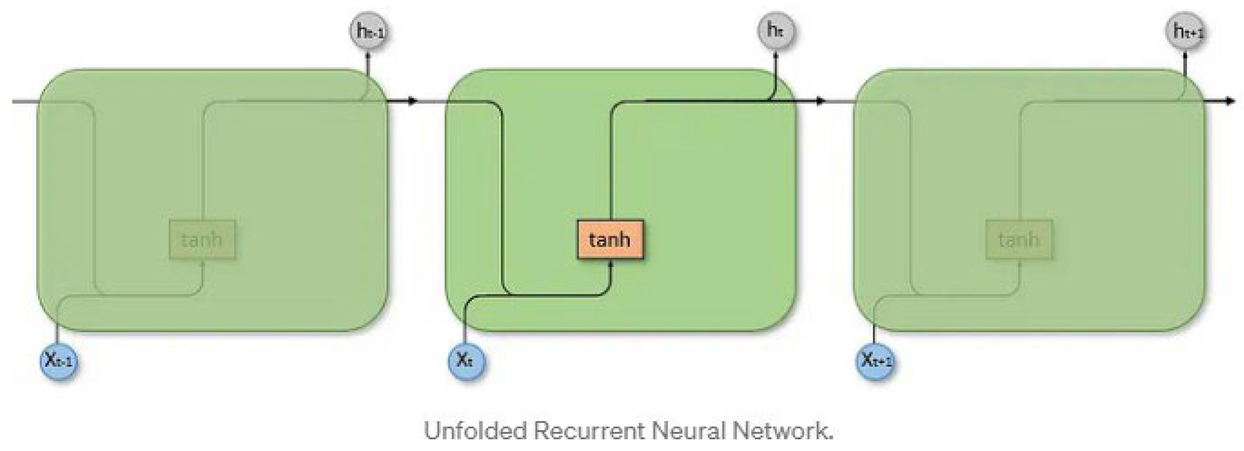
RNNs are designed to handle sequential data. Unlike traditional feedforward ANNs, where data flows in a one-way direction from input to output, RNNs introduce feedback loops that allow information to persist across time (Zargar, 2021). In the context of this paper, RNNs allow for the possibility of better prediction by not just relying on a single frame but utilizing multiple frames. In practice, more advanced iterations of RNNs, such as LSTMs and the inclusion of attention, have proved very successful and significantly outperformed basic RNNs (Sherstinsky, 2020). This paper will consider these advanced models. Figure 5 depicts a simple illustration of the RNN architecture.

This example depicts a sequence of 3 inputs (X_t − 1, X_t, X_t + 1) used to make a prediction. In the context of this paper, a sequence of frames of a single animal could be the input. At time point t, the neural network takes two inputs, X_t and X_h − 1. For example, this could refer to the input frame at time t (X_t) and the memory maintained from the previous frames (X_h − 1). This trend continues until the end of the sequence is reached before finally making a prediction that has been able to utilize information from each frame. Due to the novelty of this paper, several different architectures will be explored. These include utilizing transfer learning, incorporating ROI (region of interest) data and multi-input architectures.

2.4. Transfer Learning

It has become increasingly common within the CV community to treat image classification not as an end in itself, but rather as a “pretext task” for training deep CNNs (Huh et al., 2016). The key idea is to allow a pre-trained model to determine good general-purpose features and then adapt these features to the user’s target task. Utilizing transfer learning in this way has become the standard for solving a wide range of CV tasks (Huh et al., 2016). One of the most prominent datasets used for transfer learning in CV is the ImageNet dataset. ImageNet contains millions of labelled images and thousands of object categories, making it an exceptional resource for training large-scale deep CNNs. The use of the ImageNet dataset has been successful in several CV sub-fields such as classification (Razavian et al., 2014), object detection (Sermanet et al., 2013), human pose estimation (Carreira et al., 2016) etc.

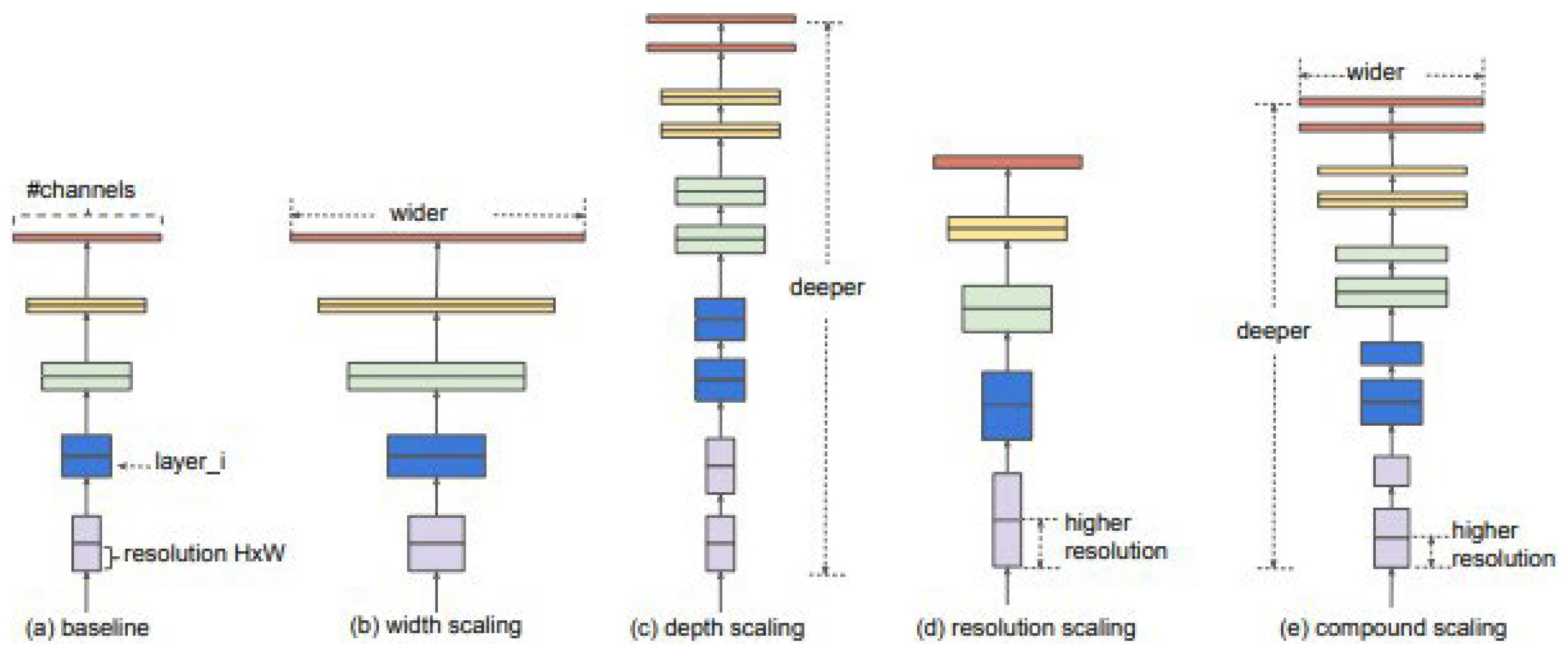
As noted in the literature review above, Gjergji et al. (2020) achieved good results using the EfficientNet models (Tan and Le, 2019). EfficientNet provides a relatively small but high-performing model (see Figure 6) when trained on ImageNet, which can be advantageous when the input dataset is relatively small and/or large compute resources are not freely available (Gjergji et al., 2020).

The novelty of the EfficientNet architecture is the scaling of the model’s depth, width, and resolution simultaneously in a principled manner. Instead of manually choosing these hyperparameters, the model instead uses a compound coefficient that systematically scales the model in a balanced way. This allows EfficientNet to find a great balance between model size and accuracy (Tan and Le, 2019)

2.5. Including Region Of Interest Data

While there are significant benefits in isolating the object of interest (animal), i.e., reducing the dimensionality of input and removing noise, drawbacks exist. One significant drawback is the potential loss of context or information when isolating the object of interest (animal) from the entire scene. This loss of context can impact the accuracy of predictions, particularly in scenarios where the target variable is continuous, such as predicting cattle weight. In this paper’s context, the animal’s distance from the camera can significantly influence its perspective in the captured image. As a result, solely focusing on the detected animal or ROI (region of interest) may lead to incomplete representations of the actual scene and negatively impact the quality of weight predictions. To address this limitation, an approach that considers the isolated object and the surrounding context might be beneficial. Integrating ROI data (ROI coordinates with respect to the original image) into the CNN could help retain valuable information about the object’s spatial relations within the entire frame and thus improve accuracy.

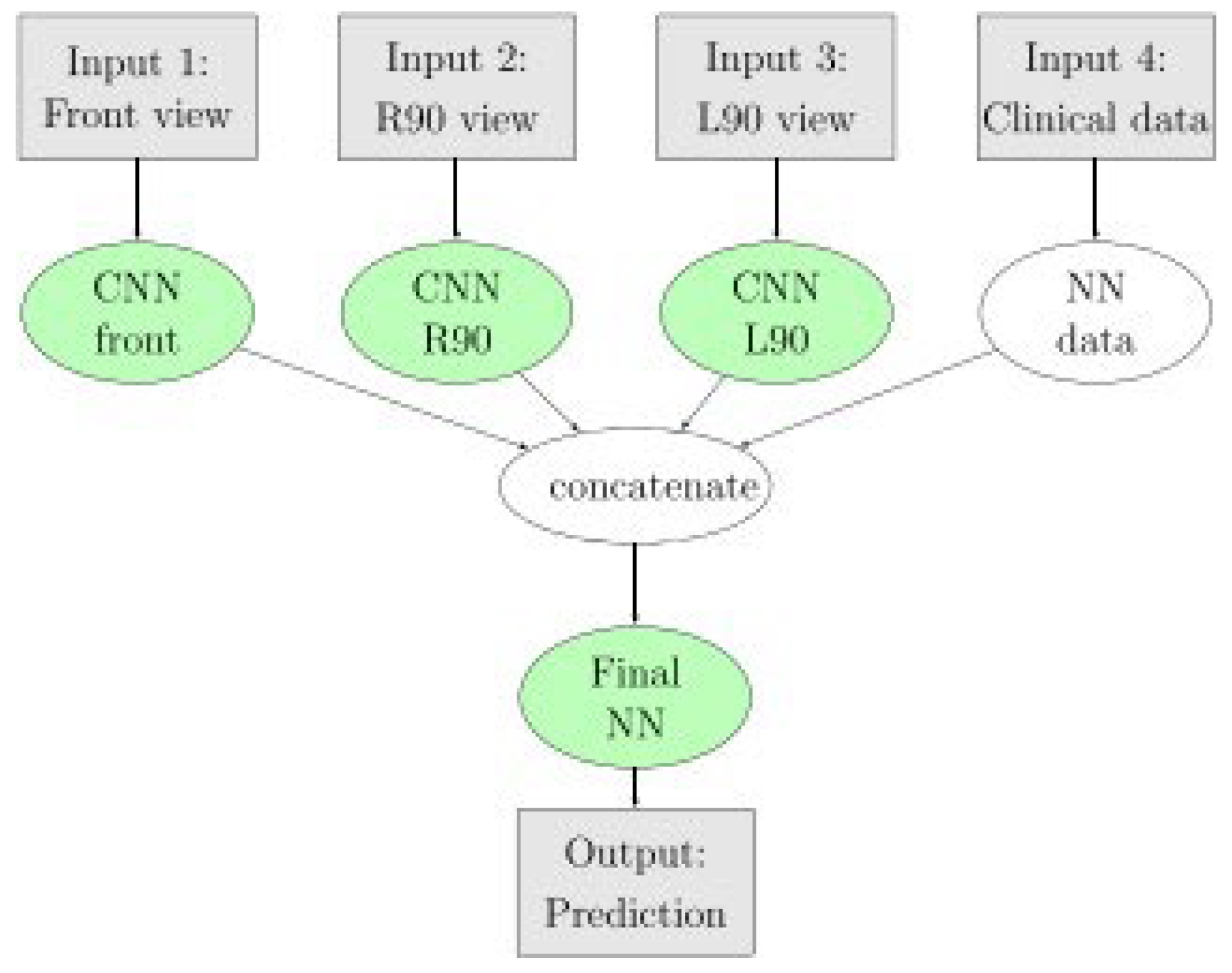
Figure 7 below depicts an architecture defined by Sánchez-Cauce et al. (2021) with impressive results in their study on breast cancer prediction. Input 4 of this architecture does not pass through a convolutional layer, but instead, a simple dense (neural network) layer before this information is concatenated with the flattened data from the image inputs. This paper will consider a similar approach.

2.6. Multi Input CNN

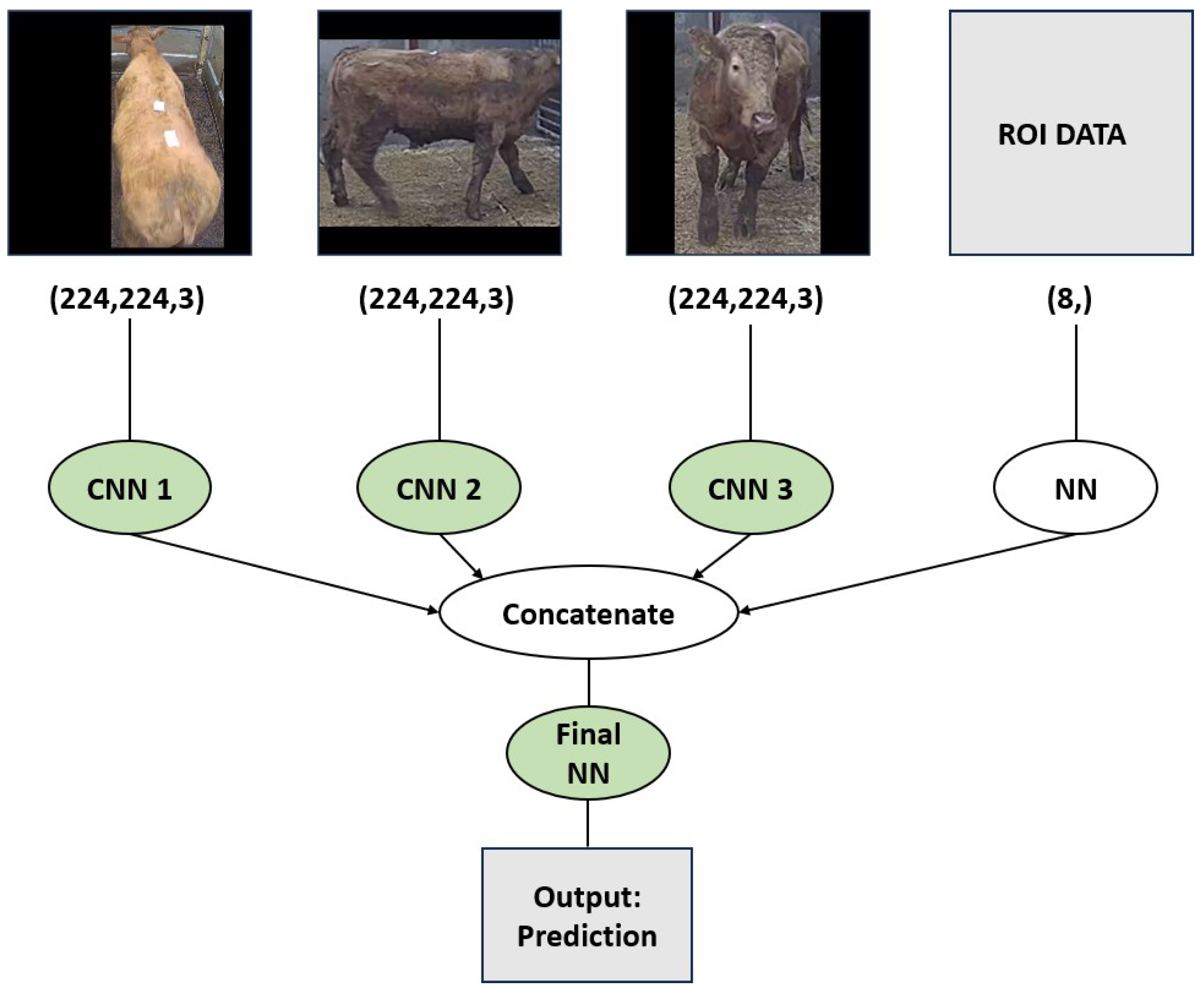
A multi-input architecture is already being considered by including the ROI data defined in the previous section. Multi-Input CNN in this context refers to multiple inputs that have their initial layers before eventually being concatenated with the other Inputs. In Figure 7 above, there exist four inputs in the defined architecture. Inputs 1-3 are images (front, left, and right views), and input 4 is clinical data (descriptive, non-image). Each input 1-3 will all have its own defined architectures, that is, an individual number of convolutional layers and node per layer, stride, pooling, padding, etc. Similar to the advantages of RNNs, this approach can benefit from utilizing multiple frames to make a single prediction. In the context of this paper, a reasonable approach may also be to include four channels (top-down, side view (wide), side view (narrow) and ROI). An example is shown in Figure 8 below.

Here frames are captured, with the object isolated, the frame resized down to 224x224 dimensions and sorted into categories (views) before being fed as inputs to the model. Note that channel 4 has a dimension of just (8), i.e., coordinates of input 2 and input 3 with respect to the original image. The animal of interest here is a 680 kg Charolais bull.

2.7. Statistical Analysis of Data

The primary evaluation method employed in this paper is the utilization of L1 loss/MAE (mean absolute error). This involves calculating the average difference between the animal’s actual weight in kilograms and the weight value predicted by each model. The MAE scores obtained from the training and validation sets will be considered. However, the ultimate measure of success will be based on the accuracy achieved on the holdout test set. The approach of 10-fold cross-validation will be explored for models that demonstrate promising performance. This technique enhances confidence in the model’s ability to effectively learn from the data. Given the significance of the work by Gjergji et al. (2020) as a foundational reference in this research, the MAE error of 23.19 kilograms achieved in their study will serve as a relevant benchmark for comparison. Although it’s important to note that direct comparison may not be entirely equitable due to various factors, it provides a meaningful indication of what can be considered a favorable outcome.

2.8. Model Implementation

The YOLO object detection algorithm is used to detect the animal of interest within the frame. The exact implementation is a custom-made YOLOV8, that is, the algorithm was trained on custom date involving 500 images per camera (top-down and side views) and is looking to detect a single object (the animal). Images were manually annotated using footage from the exact location of the dataset. MakeSense.AI (Skalski, 2023) was the application used to annotate the training data, and the Python package ‘ultralytics’ (Jocher et al., 2023) was used to train the custom YOLOV8 algorithm, given the custom annotated set.

Several pre-processing steps are required before training a model can commence. The initial dataset consists of three lengthy videos, each featuring a varying number of animals (68, 80, and 92), accompanied by associated metadata. This metadata includes the timing of animal entries into each view and their corresponding weights in kg. It is important to note that preliminary data clean-up and general data quality validation were conducted on the original data. Next, the larger videos were divided into individual clips per animal.

As CV methodologies rely on frames/images as inputs, converting each clip into images is essential. However, not all frames within each clip are valuable; in fact, many frames need to be discarded due to the presences of multiple animals in the frame, a “noisy” frame where a human may obstruct the camera view, or the entire or fraction of animal out of frame.

These issues and the need to select specific frames per video for utilization in CV models can be effectively addressed by implementing object detection algorithms using the custom-made and pre-trained YOLO models. The following is a simplified logic flow used to create the CV model inputs:

Once each clip has been processed and useful frames extracted, the next step is to process each image as input for training a deep learning model. This involves defining what animals to be used in training, validation and testing sets, normalizing pixel values, and validating that results are as expected. Figure 9 depicts a random sample of 25 processed images (223,224,3) ready for training.

Following the processing of the 480 videos (240 per view), 1280 images are saved from the top- down view and 18,696 images are saved from the side view. It is important to note that derived images are a function of the constraints placed on what is deemed an acceptable image to be used in training. Such constraints were determined via trial and error. The associated code is available from the authors on request. Note that the actual code applies additional constraints to what frames are deemed acceptable. This includes minimum and maximum ROI height, width and ratio constraints.

Fitting deep learning models to predict the weight of individual animals/bulls is the final step in the workflow. The following is an overview of all the necessary steps that have been outlined to reach this final stage:

Gather raw data, including three extensive video files from three market sales, each accompanied by relevant metadata.
Transform the raw video files into distinct clips for each animal within the dataset, covering both views.
Develop a custom YOLO object detection algorithm to identify the target object (cattle) within the clips.
Integrate a pre-trained YOLO object detection algorithm that detects humans, thereby eliminating extraneous noise.
Establish criteria to determine which frames should be incorporated into the deep learning models.
Define required functions and specify the desired output image size (224, 224, 3) to convert original frames into transformed training images.
Utilize the procedures outlined in steps 3 to 6 to iterate through each clip and extract transformed images, subsequently employed in training the deep learning models.
Perform required data transformations and partition the data into training, testing, and validation sets.

Completing the eight defined steps is a prerequisite before commencing the model fitting process to estimate the weight of Irish livestock.

3. Results

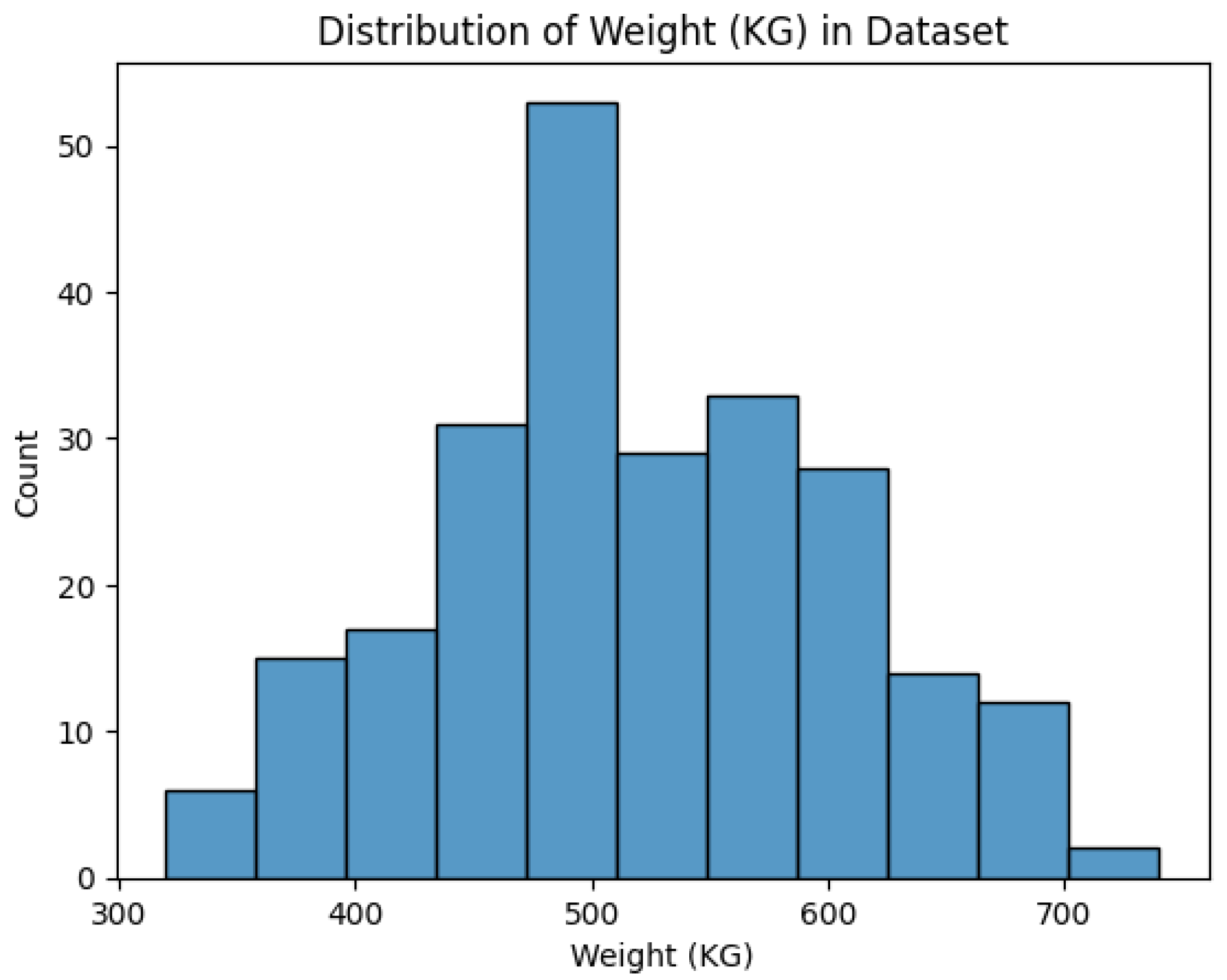
The dataset contains 240 cattle, all of which are bulls (male). The weight of these animals ranges from 320-740 kg, with a mean of 520 kg. The dataset is approximately normally distributed and contains 16 different breeds of bulls, the majority of which are Angus (51), Limousin (45), Charolais (32), Freisian (27), Hereford (17), Simmental (15), Belgian Blue (14) and Holstein (13). There is a variable amount of footage captured per animal per view. This ranges from 5-72 seconds of footage, with an average of 25 seconds captured per view per camera.

Figure 10. Distribution of Weight (kg) in Dataset.

The results are summarized in Table 1 and discussed below.

3.1. Top-Down View Predictions

Two distinct architectural approaches were explored during the development of the top-down view prediction models: 1) CNNs and 2) RNNs. It’s worth noting that while several implementations were experimented with, only the most significant architecture designs and corresponding results will be discussed.

Both transfer learning and models developed from scratch were tested. However, it is noteworthy that the transfer learning models demonstrated relatively poor performance. As a result, the subsequent analysis and reporting will predominantly focus on the models developed from scratch. It is important to note that the top-down view has a much more limited distribution of the types of images deemed acceptable, i.e., all images in this set adopt a uniform top-down perspective of the animal, with the subject gazing directly ahead. The original images also underwent limited cropping, eliminating peripheral left and right views. This type of cropping renders the inclusion of Region of Interest (ROI) data redundant as the ROI is already contained. As a result, the multi-input architecture outlined above is not considered.

3.2. CNN - Model 1

This model has 895 training images and 188 and 197 testing and validation images, respectively. As the model employed is quite complex relative to the number of training examples, regularization was employed via dropout and L2 regularization to avoid overfitting to the training data. The optimal weights were determined via the validation set performance such that this accuracy was similar to that attained in the training set. Note that data augmentation was also explored, but this did not improve model performance.

After some hyper-parameter tuning, the optimal weights were achieved via a validation MAE of 46 kg. This resulted in a testing MAE of 52 kg with a corresponding R² of 0.525.

3.3. RNN - Model 2

Model 2 adopts a hybrid architectural approach by integrating CNN and RNN elements. Although RNNs are predominantly designed to process sequential data in vectorized form, they are unsuitable for handling raw image data. In contrast, CNNs are well-suited for image data processing due to their adeptness at capturing spatial features. In this hybrid model, CNNs extract pertinent feature vectors from images. Subsequently, these extracted feature vectors are fed into RNNs, capable of processing feature sequences and making predictions. This combi- nation of CNNs and RNNs facilitates a comprehensive analysis of image-based data, effectively harnessing both spatial and sequential attributes to enhance predictive performance.

Given that the CNN component (Model 1) has already been developed, the RNN in Model 2 can conveniently leverage the feature vectors extracted from the optimized CNN. Specifically, the flattened vector resulting from the final convolutional layer in Model 1, with dimensions (64, 28, 28), will serve as the input for the RNN. Notably, this input will consist of three images (in sequence) represented by their respective feature vectors. Note that although several RNN architectures were trialed, the final architecture reported on is an LSTM model that utilizes attention. Unfortunately, the RNN (LSTM) model could not outperform the original CNN model. Training MAE could not break 50 kg, while Validation and Testing MAE achieved similar values. This is likely due to the additional data requirement associated with the more complex RNN architecture.

3.4. Side View Predictions

Multiple strategies were trialed to explore side-view predictions. For simplicity, this section is organized into two categories, 1) Architectures that leveraged single-image inputs for training and 2) Architectures that utilized dual image inputs for training. All models trialed incorporate the object detection ROI coordinates. As in the top-down view architectures described in above, a comprehensive investigation involving transfer learning and models built from the ground up was conducted. However, it’s noteworthy that the attempts with transfer learning once again yielded unsatisfactory results. As a result, the subsequent analysis will explore models developed from scratch.

3.5. Single Image with ROI (2 Input Model) - Model 3

Of the 240 animals/clips that make up this dataset, 18,696 images were deemed appropriate for inclusion after processing of video and transformation. 70% of cattle were used for training (13,166 images) and 15% for both testing (2,903 images) and validation (2,627 images). The results obtained from this architecture could only achieve a MAE of 60kg on the testing set. It is important to note that by simply predicting the average weight in the training set, you would attain a MAE of 73kg. In reaching this result, there were three methods were trialed:

9.: Single Image without ROI Coordinated: This preliminary approach achieved a MAE of 72kg on the test set.
10.: Single Image without ROI with Data Augmentation: Incorporating data augmentation techniques led to a performance boost, resulting in a MAE of 66kg on the test set.
11.: Single Image with ROI: Including Region of Interest (ROI) coordinates further refined the model, achieving a MAE of 65kg on the test set.
12.: Final Iteration - Single Image with ROI and Data Augmentation: The final configuration, amalgamating ROI coordinates and data augmentation, culminated in a MAE of 60kg on the test set.

Although the results achieved in this section are underwhelming, it depicts that some learning has occurred. Moreover, the addition of the ROI coordinates and data-augmentation improves accuracy.

3.6. Dual Image with ROI (4 Input Model) - Model 4

The methodology behind this approach involved categorizing images based on the width-to-height ratio of the ROI. Specifically, images with a width/height ratio greater than 1 were categorized as “wide,” while images with a height/width ratio greater than 1 were classified as “narrow.” By employing a random permutation technique for both wide and narrow images, the resulting dataset was composed of 39,662 sets of images for training. The validation and testing sets comprised 8,517 and 7,924 images, respectively. Drawing parallels to the outcomes observed in Model 2, where incorporating a RNN introduced additional complexity without a commensurate increase in training examples; this four-input model failed to surpass the performance achieved by the Single Image iteration detailed in the previous section. The final MAE achieved on testing was 63kg.

3.7. Combination Top-Down and Side View Predictions

The final model trialed uses the side-view and top-down view images in parallel. The previous models clearly show that the top-down view is a better predictor of weight. As a result, Input 5 (top-down input) was the input given the most weight. Similar to the approach taken in Model 4, several permutations of top-down, wide and narrow image sets determined the input (with ROI coordinates for Input 1 and Input 3). This final model achieves the best results with a MAE of 35kg (and an R² of 0.6) on the testing set. It is important to note that this coincides with an MAE of 42kg on training and 45kg on validation, and as a result, this test set accuracy is overly optimistic. Nevertheless, a consistent MAE of less than 45kg across training, validation and testing sets is the best accuracy achieved in this study.

4. Discussion

The paper contributes to the current body of literature surrounding the CV weight estimation of cattle. It addresses several gaps in the current literature while testing to what extent CV can be useful. This paper offers contributions to the literature including a mechanism to control for dataset noise due to in-motion cattle images and the use of image data collected during an active cattle auction. Other unique features of this analysis include the simultaneous use of both side-view and top-down imagery and the use of object detection algorithms to limit the impact of extraneous image features e.g., humans. This paper successfully develops a multi-step process where two custom object detection algorithms were successfully developed, and intricate logic was utilized to process each video frame by frame in order to retain useful images for modelling. The results demonstrate new insights into CV applications in the context of animal weight estimation. The discussion that follows focuses on methods for training data which has excessive variability in its input without the required data quantity to achieve reasonable results, i.e., 240 animal dataset is much too small for a problem of this complexity.

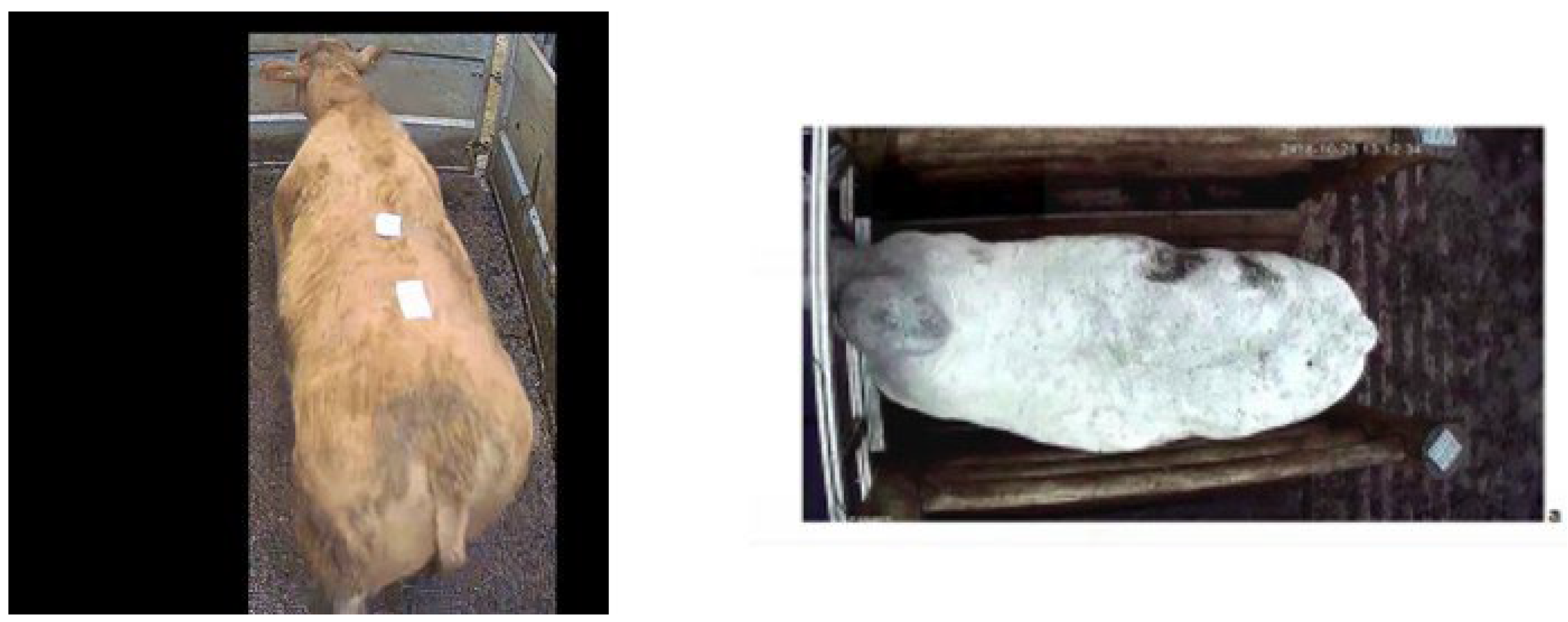
Each of the trialed model types elicited unique and interesting results. The top-down view substantially outperformed the side view. However, it achieved accuracy levels that were lower than those reported in the previous literature. Potential reasons may be that the camera is not directly above the animal, but rather at an angle. There is also significant variability in the images captured as the animal is allowed to roam and there is a large distribution of cattle breeds within the sample dataset. Figure 11 below depicts an example of the input used in this paper (left) and that used by Gjergji et al. (2020) (right) who employ a view directly above the animal and capture a much more standardized view, i.e., the animal cannot roam.

This research provides new insights around the setting of parameters to accept or reject an image for analysis. The approach used here determined that more data (consisting of increased variability between inputs) performed worse than just allowing a strict subset for inclusion. Even though it resulted in a much smaller subset of data, quality images were preferred over a larger quantity of images with a large range of variability. This is a significant result and further emphasizes the requirement for the strict standardization of inputs to achieve accurate results in CV regression tasks. It is not unreasonable to believe that substantially increasing the size of this dataset would result in comparable results to Gjergji et al. (2020).

The side-view predictions performed poorly overall. The issues surrounding the lack of standardization discussed in the top-down view are further exasperated with the side-view predictions. This small sample of inputs shows that the variability/lack of standardization is substantial.

The final models trialed used both side and top-down views in parallel in a multi-input architecture. While this final model performed the best, the drawbacks of the earlier models remain. The current paper supports earlier research by demonstrating that the top-down view can be a good predictor. This paper suggests that in the correct context, the addition of a standardized side-view to be used in parallel could bolster this accuracy.

The results of this study highlight the limitations of CV and the requirement for appropriate data quantity given problem complexity, i.e., lack of standardization in inputs for CV tasks. This study also suggests that much more complex model architectures are required, and such architectures require much more data. However, CV can provide somewhat reliable weight estimates in cattle despite the poor accuracy obtained in certain CV models. The most accurate CV implementations utilizing standard imaging can achieve a MAE accuracy of approximately 23kg which can be of value in certain use cases. The final hurdle for CV weight estimates is in terms of generalization. Moreover, the extent to how well these CV models can generalize to new environments still needs to be tested.

This paper underscores the complexity of the CV generalization problem. Moreover, in order to achieve generalizable results, a large number of animals/training data is required (much greater than the 240 animals in this study). This study also suggests that the lack of motion and increased standardization of inputs will likely result in more accurate results.

The current paper was initially motivated to determine the feasibility of creating a phone application where the user would capture a video of cattle and could obtain a reasonable estimate of that animal’s weight. This could have significant economic benefits by potentially lowering transaction costs associated with time and effort in transporting livestock from the seller’s location to a centralized market to be weighed before being transported to the buyer’s location. The current paper outlines the challenging procedure to solve such a problem. Implementation would require a considerably large dataset and large computing and memory resources to process and fit such an implementation. Additionally, higher-quality imaging equipment may be a prerequisite for such an application’s success.

4.1. Limitations and Future Work

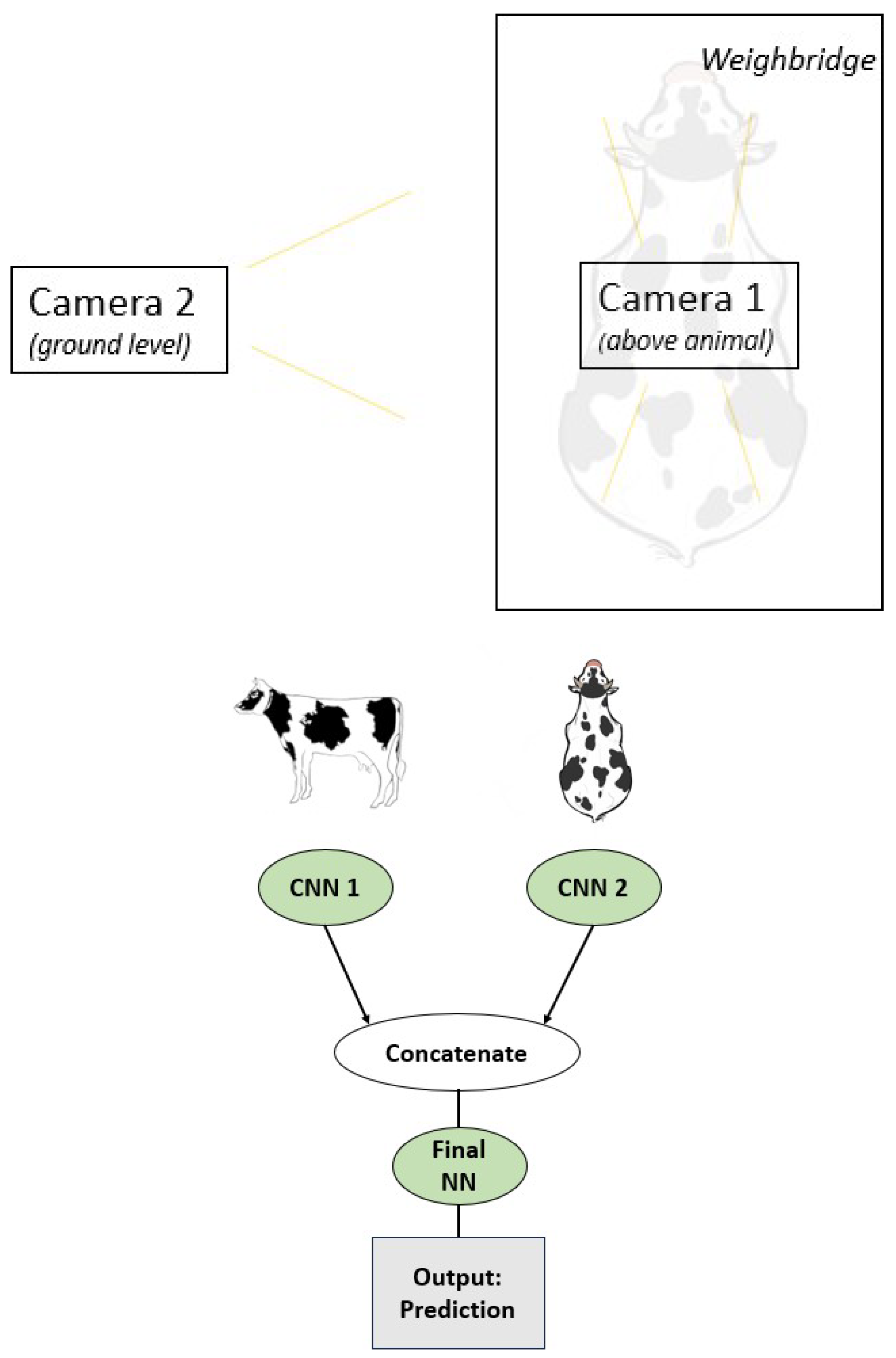
While the multi-step data flow developed this paper works quite well, higher model accuracy could be achieved if the feed-in dataset was enhanced. The following section outlines the key lessons learned from this study to recommend how an enhanced dataset could be collected and processed. Figure 12 proposes an improved data collection strategy. Similar to this study, there are two views (side and top-down). However, unlike this study, both views are captured simultaneously. Camera 1 should be placed directly over the midpoint of the animal once they enter the weighbridge. Moreover, the weighbridge should be wide enough to accommodate each animal and narrow enough to ensure the animal cannot roam freely. The accuracy of the weighbridge should be able to achieve weights to the nearest kg (or better). Camera 2 should be placed on ground level (animal level) and in line with camera 1 (center of animal). Unlike the dataset used in this study, the variability allowed via this setup is significantly reduced. It is an obvious conclusion that relying solely on a single 2D view is losing much of the information required to obtain accurate weight estimates. Utilizing both sides and top-down in a standardized fashion, could yield promising results. Lastly, a large dataset with varied breeds and weight distribution is preferred to maximize the generalizability of such data collection.

4.2. Contribution

The primary contribution of the current paper is in creating a robust data pipeline which uses as inputs sizeable raw video files and, by using several interoperable technologies, including pre-trained and custom object detection algorithms, transforms video into appropriate feed-in data to train deep learning models. It contributes to the literature by demonstrating the limitation of CV for regression problems and the requirement for large datasets, especially when considering a complex problem where the inputs have much variability. There is a clear requirement for large datasets which incorporate more than a single view in a standardized fashion to further the field of research. For this technology to become mainstream, studies must report much-improved accuracy and demonstrate the ability to generalize well to new environments. Only then can one expect farmers to embrace CV methods and, in turn, relinquish their tried and trusted tape measures.

Author Contributions

Writing – original draft, methodology, formal analysis. J. Garvey: Writing – review and editing, supervision, implications, conceptualization. F. O’Brien: Conceptualization, supervision, methodology. E. Knapp: Writing – review and editing.

Funding

This research received no specific grant from any funding agency, commercial, or not-for-profit organization.

Data Availability Statement

The data that support the study findings are available from the corresponding author upon request.

Conflicts of Interest

The authors declare no conflicts of interest involved in this study. Declaration of Generative AI and AI-Assisted Technologies in the Writing Process: The authors declare that no AI or AI-assisted technologies were used during the writing of this work. Makesense.ai (Skalski, 2023) was used to annotate the model training data as part of the data preparation for this study.

References

Berry, D.P. , Buckley, F., Dillon, P., Evans, R.D., Rath, M., Veerkamp, R.F., 2002. Genetic parameters for level and change of body condition score and body weight in dairy cows. Journal of Dairy Science, 85, 2030–2039. [CrossRef]
Brandl, N. , Jørgensen, E., 1996. Determination of live weight of pigs from dimensions measured using image analysis. Computers and Electronics in Agriculture, 15, 57-72. [CrossRef]
Brody, S. , Davis, H.P. and Ragsdale, A.C., 1937. Growth and development with special reference to domestic animals. XLI, Relation between live weight and chest girth in dairy cattle of unknown age. University of Missouri, College of Agriculture, Agricultural Experiment Station.
Carreira, J. , Agrawal, P., Fragkiadaki, K., Malik, J., 2015. Human Pose Estimation with Iterative Error Feedback. 2016 IEEE Conference on Computer Vision and Pattern Recognition (CVPR), 4733-4742.
Chougule, S. , Koznek, N., Ismail, A., Adam, G., Narayan, V., Schulze, M. 2019. Reliable Multilane Detection and Classification by Utilizing CNN as a Regression Network. In: Leal-Taixé, L., Roth, S. (eds) Computer Vision – ECCV 2018 Workshops. ECCV 2018. Lecture Notes in Computer Science(), vol 11133. Springer, Cham. [CrossRef]
Cominotte, A. , Fernandes, A. F. A., Dorea, J. R. R., Rosa, G. J. M., Ladeira, M. M., Van Cleef, E. H. C. B.,... & Neto, O. M. 2020. Automated computer vision system to predict body weight and average daily gain in beef cattle during growing and finishing phases. Livestock Science, 232, 103904.
Danker, J. 2022. A brief introduction to recurrent neural networks. Available at: https:// towardsdatascience.com/a-brief-introduction-to-recurrent-neural-networks-638f64a61ff4.
Domecq, J.J. , Skidmore, A.L., Lloyd, J.W., Kaneene, J.B., 1997. Relationship between body condition scores and conception at first artificial insemination in a large dairy herd of high yielding Holstein cows. Journal of Dairy Science, 80, 113–120. [CrossRef]
Enevoldsen, C. , Kristensen, T., 1997. Estimation of body weight from body size measurements and body condition scores in dairy cows. Journal of Dairy Science, 80, 1988–1995. [CrossRef]
Fang, B. , Klabjan, D., 2019. Convergence analyses of online Adam algorithm in convex setting and two-layer ReLU neural network. arXiv preprint. arXiv:1905.09356.
Fernández-Carrión, E. , Barasona J.Á., Sánchez, Á., Jurado, C., Cadenas-Fernández E., Sánchez-Vizcaíno, J.M., 2020. Computer Vision Applied to Detect Lethargy through Animal Motion Monitoring: A Trial on African Swine Fever in Wild Boar. Animals, 10, 2241. [CrossRef]
Gjergji, M. , de Moraes Weber, V., Ot’avio Campos Silva, L., da Costa Gomes, R., Luis Alves Campos de Arau´jo, T., Pistori, H., Alvarez M., 2020. Deep learning techniques for beef cattle body weight prediction. International Joint Conference on Neural Networks (IJCNN), July.
Grandin, T. , Shivley, C., 2015. How Farm Animals React and Perceive Stressful Situations Such As Handling, Restraint, and Transport. Animals: an open access journal from MDPI, 5, 1233–1251. [CrossRef]
Hansen, M.F. , Smith, M.L., Smith, L.N., Abdul Jabbar, K., Forbes, D., 2018. Automated monitoring of dairy cow body condition, mobility and weight using a single 3D video capture device. Computers in Industry, 98, 14–22. [CrossRef]
Heinrichs, A.J. , Rogers, G.W., Cooper, J.B., 1992. Predicting body weight and wither height in Holstein heifers using body measurements. Journal of Dairy Science, 75, 3576–3581. [CrossRef]
Huh, M. , Agrawal, P., Efros, A.A., 2016. What makes imagenet good for transfer learning? arXiv preprint. arXiv:1608.08614.
Jiang, P. , Ergu, D., Liu, F., Cai, Y., Ma, B., 2022. A Review of Yolo Algorithm Developments. Procedia Computer Science, 199, 1066–1073. [CrossRef]
Jocher, G. , Chaurasia, A., Qiu, J., 2023. Ultralytics yolov8. Available at: https://github. com/ultralytics/ultralytics.
LeCun, Y. , Bengio, Y., Hinton, G., 2015. Deep learning. Nature, 521(7553), 436–444. [CrossRef]
Lesosky, M. , Dumas, S., Conradie, I., Handel, I.G., Jennings, A., Thumbi, S., Toye, P., Bronsvoort, B.M., 2013. A live weight-heart girth relationship for accurate dosing of east African shorthorn zebu cattle. Tropical Animal Health and Production, 45, 311–316. [CrossRef]
Meer, P. , Mintz, D., Rosenfeld, A., Kim, D.Y., 1991. Robust regression methods for computer vision: A review. International Journal of Computer Vision, 6, 59-70. [CrossRef]
Mushtaq, A. , Qureshi, M.S., Khan, S., Habib, G., Swati, Z.A., Rahman, S.U., 2012. Body Condition Score as a Marker of Milk Yield and Composition in Dairy Animals. Journal of Animal and Plant Sciences, 22, 169-173. [CrossRef]
Nabokov, V. , Novopashin, L., Denyozhko, L., Sadov, A., Ziablitckaia, N., Volkova, S., Speshilova, I., 2020. Applications of feed pusher robots on cattle farming and its economic efficiency. International Transaction Journal of Engineering, Management, & Applied Sciences & Technologies, 11:1–7.
Oliveira, D.A.B. , Pereira, L.G.R., Bresolin, T., Ferreira, R E.P., & Dorea, J.R.R., 2021. A review of deep learning algorithms for computer vision systems in livestock. Livestock Science, 253, 104700.
Ozkaya, S. , Bozkurt, Y., 2009. The accuracy of prediction of body weight from body measurements in beef cattle. Archives Animal Breeding, 2009, 52, 371–377. [CrossRef]
Ozkaya, S. , 2013. The prediction of live weight from body measurements on female holstein calves by digital image analysis. The Journal of Agricultural Science, 151, 570–576. [CrossRef]
Pethick, D.W. , Hocquette, J.F., Scollan, N.D., Dunshea, F.R., 2021. Review: Improving the nutritional, sensory and market value of meat products from sheep and cattle. Animal : an international journal of animal bioscience, 15, Suppl 1, 100356. [CrossRef]
Qiao, Y. , Kong, H., Clark, C., Lomax, S., Su, D., Eiffert, S., & Sukkarieh, S., 2021. Intelligent perception for cattle monitoring: A review for cattle identification, body condition score evaluation, and weight estimation. Computers and Electronics in Agriculture, 185, 106143.
Razavian, A.S. , Azizpour, H., Sullivan, J., Carlsson, S., 2014. CNN Features Off-the-Shelf: An Astounding Baseline for Recognition. 2014 IEEE Conference on Computer Vision and Pattern Recognition Workshops, 512-519.
Redmon, J. , Divvala, S.K., Girshick, R.B., Farhadi, A., 2016. You Only Look Once: Unified, Real-Time Object Detection. IEEE Conference on Computer Vision and Pattern Recognition (CVPR), 779-788.
Rezende, M. P. G. , Malhado, C. H. M., Biffani, S., Carrillo-Tabakman, J. A., Fabbri, M. C., Crovetti, A., Carneiro, P. L. S., & Bozzi, R., 2022. Heritability and genetic correlation of body weight and Kleiber ratio in Limousin and Charolais beef cattle breeds. Animal : an international journal of animal bioscience, 16(5), 100528. [CrossRef]
Roche, J.R. , Kay, J.K., Friggens, N.C., Loor, J.J., Berry, D.P., 2013. Assessing and managing body condition score for the prevention of metabolic disease in dairy cows. The Veterinary clinics of North America. Food Animal Practice, 29, 323–336. [CrossRef]
Roth, A.E., 2018. Marketplaces, Markets, and Market Design. American Economic Review, 108, 1609-58. [CrossRef]
Sánchez-Cauce, R. , Pérez-Martín, J., Luque, M., 2021. Multi-input convolutional neural network for breast cancer detection using thermal images and clinical data. Computer methods and programs in biomedicine, 204, 106045. [CrossRef]
Sathe, P.M. , Venitz, J., 2003. Comparison of neural network and multiple linear regression as dissolution predictors. Drug Development and Industrial Pharmacy, 29, 349–355. [CrossRef]
Sermanet, P. , Eigen, D., Zhang, X., Mathieu, M., Fergus, R., LeCun, Y., 2013. OverFeat: Integrated Recognition, Localization and Detection using Convolutional Networks. CoRR, abs/1312.6229.
Sharma, S. , Sharma, S., Athaiya, A., 2017. Activation functions in neural networks. Towards Data Science, 6, 310–316. http://www.ijeast.com.
Sherstinsky, A. , 2020. Fundamentals of recurrent neural network (rnn) and long short-term memory (lstm) network. Physica D: Nonlinear Phenomena, 404, 132306. [CrossRef]
Skalski, P. 2023. makesense.ai. (alpha). Available at: https://makesense.ai.
Tan, M. , Le, Q.V., 2019. EfficientNet: Rethinking Model Scaling for Convolutional Neural Networks. ArXiv, abs/1905.11946.
Tasdemir, S. , Ozkan, I. A., 2019. ANN approach for estimation of cow weight depending on photogrammetric body dimensions. International Journal of Engineering and Geosciences, 4:36–44. [CrossRef]
Vapnik, V. , Levin, E., Le Cun, Y., 1994. Measuring the vc-dimension of a learning machine. Neural computation, 6, 851–876. [CrossRef]
Vedaldi, A., Lenc K., 2015. Matconvnet: Convolutional neural networks for Matlab. In Proceedings of the 23rd ACM international conference on Multimedia, 689–692.
Wang, Z., Shadpour, S., Chan, E., Rotondo, V., Wood, K.M., Tulpan, D., 2021 Asas-nanp symposium: Applications of machine learning for livestock body weight prediction from digital images. Journal of Animal Science, 99, skab022. [CrossRef]
Wangchuk, K. , Wangdi, J., Mindu, M., 2018. Comparison and reliability of techniques to estimate live cattle body weight. Journal of Applied Animal Research, 46:349–352. [CrossRef]
Wathes, D. , Fenwick, M., Cheng, Z., Bourne, N., Llewellyn, S., Morris, D., Kenny, D., Murphy, J., Fitzpatrick, R., 2007. Influence of negative energy balance on cyclicity and fertility in the high producing dairy cow. Theriogenology, 68, S232–S241. [CrossRef]
Weber, V.A. , Weber, F.D., Gomes, R.D., Oliveira, A.D., Menezes, G.V., Abreu, U.G., Belete, N.A., Pistori, H., 2020. Prediction of Girolando cattle weight by means of body measurements extracted from images. Revista Brasileira De Zootecnia, 49. [CrossRef]
Weinstein, B.G. , 2018. A computer vision for animal ecology. Journal of Animal Ecology, 87, 533–545. [CrossRef]
Ying, X. , 2019. An overview of overfitting and its solutions. Journal of physics: Conference series, volume 1168, page 022022. IOP Publishing.
Zargar, S. , 2021. Introduction to sequence learning models: Rnn, lstm, gru. Department of Mechanical and Aerospace Engineering, North Carolina State University, Raleigh, North Carolina, 27606.
Zheng, Q. , Yang, M., Yang, J., Zhang, Q., Zhang, X., 2018. Improvement of generalization ability of deep cnn via implicit regularization in two-stage training process. IEEE Access, 6:15844–15869.

Figure 1. Data Collection; Top-down view.

Figure 2. Data Collection; Side view (people in frame removed).

Figure 3. YOLO Algorithm (Redmon et al., 2016).

Figure 4. Basic CNN Architecture (Vedaldi and Lenc, 2015).

Figure 5. Basic Unfolded RNN Architecture (Danker, 2022).

Figure 6. EfficientNet Architecture (Tan and Le, 2019).

Figure 7. Multi Input CNN with the addition of descriptive attributes (Sánchez-Cauce et al., 2021).

Figure 8. Example Multi Channel Architecture.

Figure 9. Sample Images for Training.

Figure 11. Paper Input vs Gjergji et al. (2020).

Figure 12. Future Work: Appropriate Modelling Architecture.

Table 1. Summary Results.

Model	Type	View	Description	MAE (KG)
1	CNN	Top-down	Single input image	52
2	RNN	Top-down	Sequence of 3 images flattened using model 1 architecture	53
3	2 input CNN	Side	Image and ROI of animal as a dual input	60
4	4 input CNN	Side	2 image input of animal with corresponding ROI’s	63
5	5 input CNN	Top-down/Side	Combination of Model 1 & 4	42

Disclaimer/Publisher’s Note: The statements, opinions and data contained in all publications are solely those of the individual author(s) and contributor(s) and not of MDPI and/or the editor(s). MDPI and/or the editor(s) disclaim responsibility for any injury to people or property resulting from any ideas, methods, instructions or products referred to in the content.

© 2024 by the authors. Licensee MDPI, Basel, Switzerland. This article is an open access article distributed under the terms and conditions of the Creative Commons Attribution (CC BY) license (http://creativecommons.org/licenses/by/4.0/).

Copyright: This open access article is published under a Creative Commons CC BY 4.0 license, which permit the free download, distribution, and reuse, provided that the author and preprint are cited in any reuse.

MDPI Initiatives

Important Links

Choose an area of interest and we will send you notifications of new preprints at your preferred frequency.

Disclaimer