1. Introduction
On September 2015, the UN General Assembly approved the 2030 Agenda, and its goals cover three dimensions of sustainable development: economic growth, inclusion, and environmental protection [
1]. By implementing these objectives, the intention is to decouple economic growth from an intensive use of resources, energy and by reducing emissions and waste from the extraction, production, consumption, and disposal of goods. The diversity of discourses related to sustainable development, the complexity and multidimensionality of the concept, and the different worldviews and values make it impossible to establish a single correct interpretation of the term. Thus, [
2] identify four interpretations of the concept of sustainable development that hinder its implementation in organizations and governments, mainly due to the disparity in interpretations of the same concept.
On the other hand, a strategic initiative was launched at the Hanover Fair in 2011 by the German Government known as Industry 4.0 [
3], which promoted a new approach aimed at empowering and transforming the manufacturing industry through the use of cyber-physical systems, the Internet of Things, and cloud computing [
4]. In parallel with the two previous initiatives, the concept of strategic asset management is developed, guaranteeing the creation and maintenance of value throughout the life cycle of the assets. Thus, the EN16646 standard [
5] shows the important relationships between operations and the maintenance of value throughout the life cycle of the physical assets.
The combination of traditional statistical tools has been used to develop prediction methods for preventive maintenance. Autoregressive moving average (ARMA) [
6], autoregressive integrated moving average (ARIMA) [
7], exponential smoothing [
8] are commonly used in statistical forecasting methods. These methods are typically limited as they rely on a sole time series, whereas methods based on deep learning are capable of incorporating numerous variables as input. This development is characterized by the use of cyber-physical systems, and although there are many definitions [
9,
10,
11,
12], all of them have in common the integration or collaboration of computer systems with physical systems (mechanical, electrical, and/or human) to perform a specific function (communication and/or control) and perform real-time calculations (analysis). Their utilization in industrial environments requires the capture, processing, analysis, and storage of huge amounts of data.
Organizations are forced to adapt to a new and changing environment as a result of the introduction of these new types of tools, which presents both opportunities and challenges. The implementation of this type of solution requires careful consideration and resolution of several difficulties, including the choice of technology to invest in, the management of current knowledge, its transfer, and the acquisition of new expertise [
13] and [
14] describes the implementation of a roadmap that optimizes the likelihood that these tools will be applied successfully.
Neural networks provide a promising solution for handling massive data [
15], and they are characterized by multiple layers that enable complex feature abstraction from data points [
16]. Industry 4.0 has the potential to transform manufacturing by enhancing flexibility, mass customization, quality, and productivity by introducing the nine pillars of industrial internet of things, big data, horizontal and vertical integration, simulations, cloud, augmented reality, autonomous robots, 3D printing, and cybersecurity. The use of high technology, and sustainability requires changes in the management of organizations, including policies and strategies within asset maintenance [
17,
18]. Moreover, [
19] indicates that smart maintenance within Industry 4.0 is oriented towards self-learning, failure prediction, diagnosis, and triggering maintenance programs. At the same time, [
20] identifies the suitability of its application since the utilization of supervised models for making forecasts will ensure that the process operates correctly and efficiently without incurring high maintenance costs and reducing product quality degradation.
Based on the aforementioned information, it can be identified that predictive maintenance is the most appropriate strategy of action in the context of Industry 4.0 and that predicting an asset’s state is essential for preventing or minimizing catastrophic failures as well as achieving the goal of zero-downtime in industrial systems [
21]. You can refer to [
22] to have a deeper understanding of the different machine learning strategies and how they connect with predictive maintenance in the context of sustainable manufacturing.
This paper aims to address the prediction of the behavior of a hydrogen compressor in the petrochemical industry, specifically in the production of caprolactam used in the manufacture of nylon 6 fibers. This is a continuous manufacturing process, which means that a failure in any component of the facility could result in the entire production being stopped. An unplanned shutdown can cause a series of unwanted inconveniences for the organization, such as possible deterioration or breakage of other manufacturing process components like sensors, control valves, and pipelines, and the potential failure to meet delivery dates for customers. It can also cause additional costs for spare parts and maintenance staff overtime. Furthermore, it is essential for control room operators to monitor the compressor’s behavior and prevent it from operating outside the pre-established working ranges for the output variable. The company’s objectives include increasing the equipment’s uptime, so the over-managers considered to use machine learning techniques to enhance the compressor’s performance and predict possible undesirable operating states.
Machine learning refers to the set of techniques and methods used by computers to autonomously extract complex patterns and relationships from large datasets and make decisions or predictions about real-world events [
23]. The concepts used in machine learning are cross-disciplinary and come from computer science, statistics, mathematics, and engineering. The main types of machine learning were outlined by [
24] as supervised learning, unsupervised learning, and reinforcement learning. Predictions are made based on new or unanticipated data [
25], unlike unsupervised learning, in which an algorithm is trained using an unlabeled dataset [
26]. Effective policies for complex tasks that typically require many interactions can be learned using reinforcement learning [
27].
Deep learning is a branch of machine learning that focuses on the learning of data representations and of hierarchical features. In order to extract features, deep learning algorithms employ a system comprising numerous layers of nonlinear processing identities (neurons) that aid in data abstraction [
28]. One of the main issues that this technique presents is distinguishing when the generated model is not overfitted to the training data and is able to generalize well when new data is presented. The difficulty in reading and comprehension of deep learning models might limit their practical application to non-qualified personnel. The primary drawbacks of using this methodology within organizations may be the management of large quantities of data, the utilization of expensive resources, necessity of large computational processing power, and a precise interpretation of the outcomes. Additionally, a sophisticated understanding of mathematical and statistical concepts is required. Due to the aforementioned factors, its implementation in small and medium-sized enterprises may prove to be challenging.
Time series prediction holds significant importance in assisting decision-makers, not only in well-known aspects such as product or service demand, but also in predicting the functioning of equipment aimed at enhancing the reliability, productivity, and quality of products or services. Hence, traditional prediction systems that are based on Industry 4.0 necessitate timely analysis and treatment of data, thereby enabling the incorporation of trained machine learning models to improve the accuracy of such predictions. Although recurrent neural networks in their various forms have traditionally been used, architectures equipped with attention mechanisms commonly used in natural language processing, which are more complex and have a higher number of trainable parameters, should provide better results [
29]. The full discussion of Transformer-based neural networks for time series prediction can be found in [
30].
Although the concepts presented in this paper are obvious to neural network specialists, they can be complex for those who are not familiar with them, making their implementation and parameterization complicated, frustrating, and sometimes impossible. Using statistical tools, this article simplifies the most innovative neural networks that can be employed and, focuses on identifying the hyperparameters of a neural network that are significant for the process of forecasting and how to adjust them to obtain adequate predictions and facilitate its replication in real-world processes.
1.1. Contribution of the Paper
A summary of recent advances in supervised learning applied to time series forecasting will help non-qualified personnel implement sophisticated neural networks in maintenance processes. The main goals of this paper are listed below:
A Transformer-based deep learning network is used to make temporal predictions about the outlet pressure of a hydrogen compressor, by utilizing compressor current consumption data as input.
Identifying the primary parameters of the neural network and their optimal settings that minimize the prediction error through the utilization of statistical tools.
1.2. Structure of the Document
The structure of this paper is as follows: The description of the origin of Industry 4.0, sustainable manufacturing and the maintenance function, and their potential use in a real-world problem have been included in
Section 1. Statistical tools that optimize the neural network are presented in
Section 2, which outlines the design of experiments. In
Section 3, the main characteristics of the facilities are detailed, as are the data gathering from the device. The short explanation of the neural network Transformer-based can be found in
Section 4, and the statistical results are described in
Section 5. Finally, the conclusions and future directions are explained in detail in
Section 6.
2. The Concepts and Procedures for the Utilization of Design of Experiments (DoE)
Most practical situations where it is intended to control the output or response of a real process are conditioned by the existence of controllable variables (factors) and other unknown factors. The DoE is a methodology proposed by Ronald A. Fisher in the 1920s and 1930s and it encompasses a set of mathematical and statistical techniques that seek the effects on a measured response variable (Y) by manipulating simultaneously some input variables (Xs).
In the application of DoE techniques, the main guidelines may include the following: (1) stating the objectives of the research, (2) defining the response variable(s), (3) determining factors and levels, (4) deciding the experimental design type, (5) conducting the experiment, (6) data analysis and (7) validation of the results. In order to estimate first and second order effects and cross-product, two-level factorial designs are used, and the polynomial function must contain quadratic terms. An orthogonal design is shown in the equation below:
where k is the number of variables,
is the constant term,
represents the coefficients of the linear parameters,
represents the variables,
represents the coefficients of the quadratic parameters,
represents the cross-product, and
is the residual associated with the experiment (random error).
The variables are usually expressed in different units and vary in different ranges, which makes it necessary to code them. If this is not accomplished, it is impossible to assess the relevance of a factor through the magnitude of the model coefficients. As a result, all factor levels are set at two levels (-1, +1) with equal spaced intervals between them.
Hence, the factorial experiments with multiple factors with two levels (“high” and “low”), suggest that the complexity of the model grows exponentially (2k), and the experiment requires a lot of resources and time. Since a low number of main effects and lower order interactions are significant to the response variable, and higher order interactions are not significant, a Fractional Factorial Design may be chosen.
The resolution of an experiment (expressed in Roman numbers) is a measure of clarity, in which the effects of factors can be estimated without confusion due to the interference of other factors. Resolution IV indicates that the no main effect or two-factor interaction is aliased with any other main effect or two-factor interaction, but two-factor interactions are aliased with three-factor interactions.
3. Description of the Equipment, Facilities, and Data Collection
A multistage (4-stages) hydrogen compressor is used to compress the gas from 0.35 kg/cm² to 285 kg/cm², cooling the hydrogen after each stage to prevent its temperature from reaching above 150 ºC (423 K). According to [
31], the present level of preventive maintenance corresponds to level 3, as there exists a monitoring and alarm system that alerts operators in the event of any anomalies, in addition to the mandatory preventive maintenance every three months.
The objective is to implement Industry 4.0 technologies with the aim of enhancing maintenance up to level 4 and reducing the over maintenance through the utilization of real-time data monitoring based on predictive techniques. The acquisition of knowledge involves the training of a neural network that employs self-attention mechanisms to identify the hyperparameter configuration that most effectively aligns with the type of data generated by the equipment. Due to the enormous volume of real-time sensor data generated in facility operations, a highly specialized distribution control system is implemented in order to enable efficient analysis and decision-making.
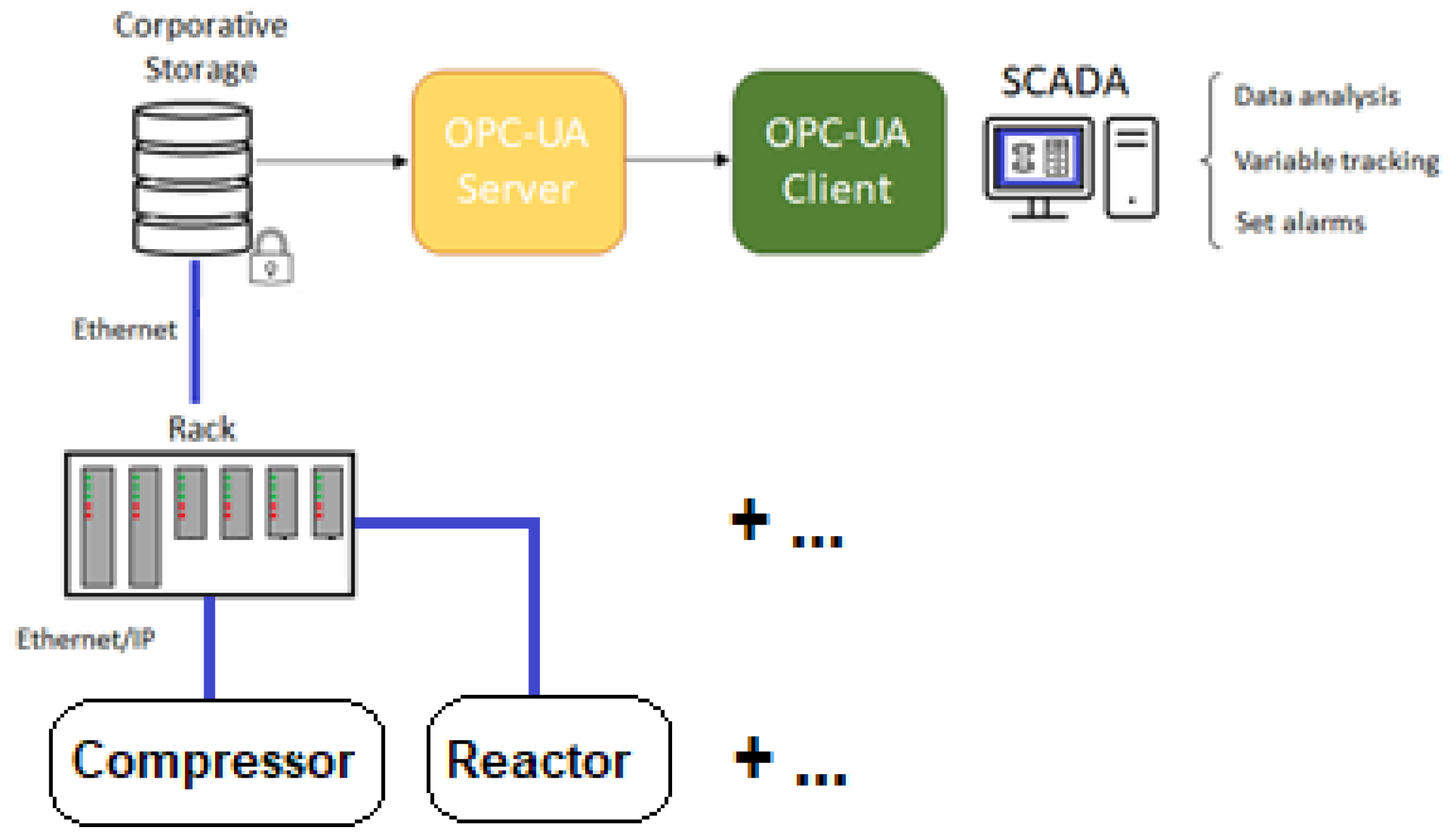
Figure 1 illustrates how data is collected through the asset’s sensors and connected via Ethernet to the control racks, which then send the signal to the unique database, which then shares the data through the OPC-UA server for subsequent processing by users. In the absence of a fog layer, the raw sensor data is transmitted directly to clients, who process the monitoring in real-time through a SCADA system and adjust variable values as required to prevent out-of-range operating situations. At present, the training processes for control operators are extensive due to the absence of any technological support for decision-making. Each action necessitates consultation with the most experienced operators until the requisite knowledge and security are acquired for a proper evaluation of the situation by trainees and to prevent the shutdown of the entire installation.
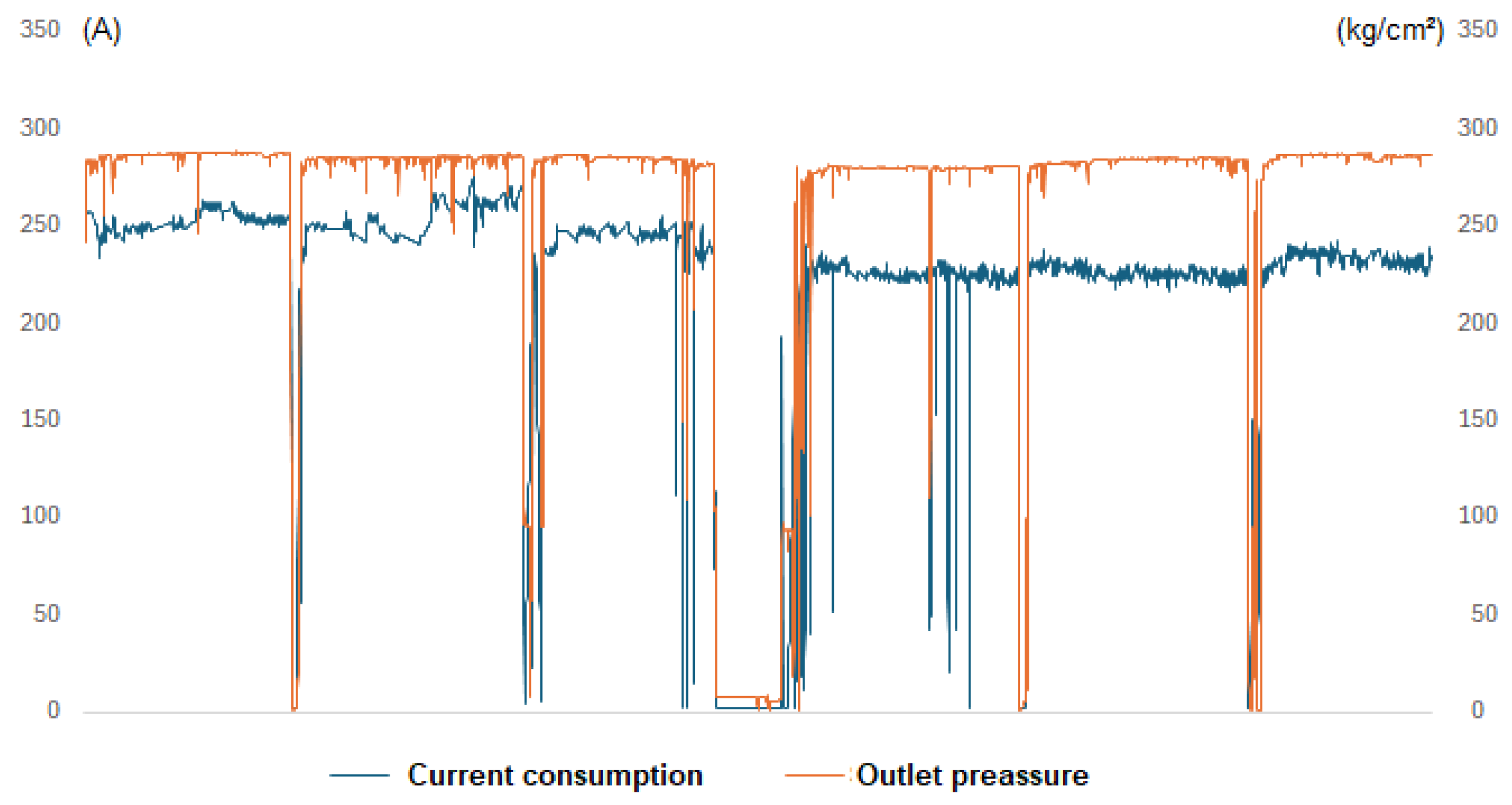
The equipment produces data points every minute, with the output pressure nominally set at 285 kg/cm² and controlled within limits of 265 and 305 kg/cm². With the objective of stabilize the process and improve the predicting capacities of the neural network, its necessary to operate on an hourly basis, and it is imperative to adjust the control limits to align with the new average values. This makes it easier to predict the next few hours of operation, as opposed to predicting the equipment’s behavior over the next few minutes. By applying the central limit theorem, the new limits have been established at 282.5 and 287.5 kg/cm² utilizing the expression σ= (305-265)/(6√60) to estimate the new standard deviation. Thus, the new limits control will be set at ±3 σ. The data depicted in
Figure 2 corresponds to the hourly average of the outlet hydrogen pressure and the current consumption by the main motor. As can be observed, there are five scheduled equipment shutdowns (preventive maintenance), and the longest stoppage occurs during the summertime.
4. Self-Attention Neural Network
The network known as Transformer, originally designed for natural language processing, uses only attention mechanisms to predict the output sequence instead of Long Short-Term Memory (LSTM) networks along with attention mechanisms of type [
32] or [
33] as were previously implemented in these types of solutions. The innovative approach of Transformers employs three distinct attention architectures: self-attention for input data in the encoder, masked attention for the predicted sequences in the decoder, and finally, cross-attention, wherein the information from the encoders and the decoders, specifically from masked attention, are combined.
The model inspired by [
34] captures dependencies between distinct points in the time sequence, although instead of employing all parts of the Transformer network, including encoders and decoders, to predict the behavior of time series values, only the self-attention mechanism of the encoder is used along a feed-forward layer to obtain the output tensor.
Therefore,
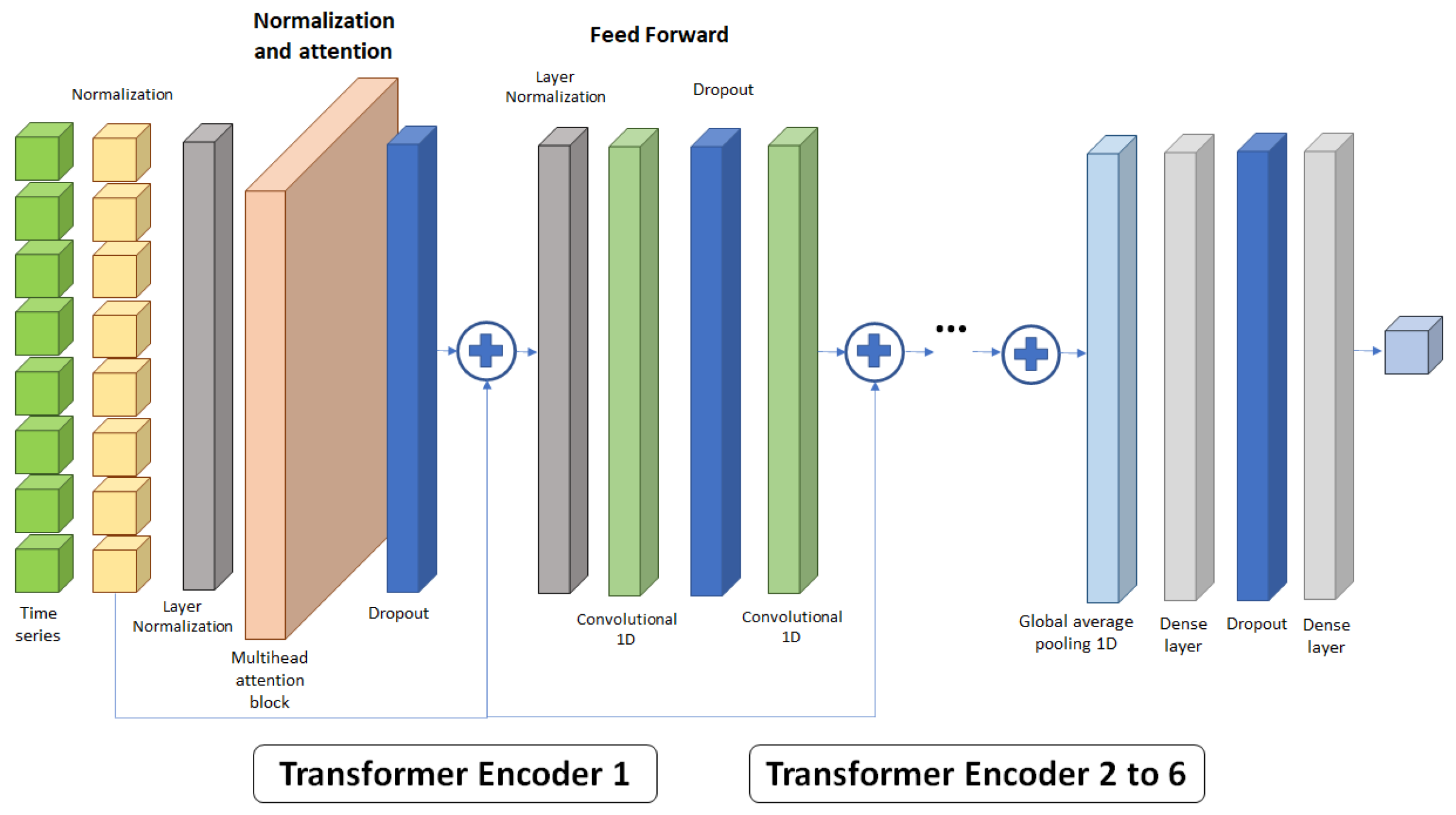
Figure 3 shows the network used, in which the normalized sequence of data to be predicted is introduced into a normalization layer before it enters multi-head attention block. Batch normalization is a regularization technique that is applied to input layers consisting of normalizing the activation values of the units in that layer so that there is a mean of 0 and a standard deviation of 1 [
35]. This improves stability and facilitates the convergence speed while avoiding problems such as exploding or vanishing gradients. You should not confuse batch normalization with input data normalization, which involves scaling input data to a specific range to improve numerical representation.
The attention block uses three independent networks: query (Q), key (K), and value (V) to acquire information from the input data and obtain a proper representation of it. The block calculates the attention weight by dividing the dot product between the query and key vectors by a scaling factor (d), transforming it using the softmax function to obtain numerical values between 0 and 1, and finally multiplying it by the value vector (Equation 3) to condense the information into a vector for each data point or token.
This set of layers and blocks forms the normalization and multi-head attention block. Multiple attention blocks can be used to detect further associations and relationships among data points and/or groups of data across different levels. These vectors are then combined using an additional neural network into a single compressed vector. Furthermore, a dropout layer is applied to its output [
36] in order to prevent excessive overfitting of the model.
The obtained vector is then added to the normalized input sequence and introduced into the Feed Forward layers, which consist of a normalization layer, a dropout layer, and two 1D convolutional layers. Finally, the output is added to the input of this layer, forming the encoder structure. Due to their feature extraction capability, convolutional networks are commonly used in data from numerical series.
Convolutional networks are a type of dense, feed-forward neural networks that have been successfully applied in many domains [
37], such as classification problems or time series classification [
38]. This structure of the model allows to recognize specific patterns and abstract information from the input sequence. This architecture is called an encoder, and it can be repeated up to six times in succession. A global average polling 1D layer (GAP1D) is added to the output of the encoders for polling, preserving all relevant information in a single layer that is easily understood by dense layers equipped with another dropout layer to obtain the time series forecast.
Once the self-attention mechanism network architecture has been defined, it is necessary to empirically analyze it and determine the value of hyperparameters that maximize the result (lower MAE or RMSE) with the lowest computational cost. Statistical analysis allows only considering relevant factors, which result in a simpler model to train.
5. Design of Experiment
This approach is based on historical data, the value of the hyperparameters is simultaneously modified to identify which ones are significant in the network’s performance, in an attempt to minimize their outputs. In this case the mean absolute error (MAE), defined by
, the root mean square error (RMSE), defined by
, the trainable number of parameters and training time, where yt is the true output, ŷt is the estimation, and T the number of data points. Many times, some type of reduction has to be selected to reduce the number of runs and save resources and computing time, since the complexity of the DoE depends on the quantity of hyperparameters considered.
Table 1 contains the factors considered in the study to determine the optimal size of the network to minimize the prediction error for the supplied data. Please note that these values are presented as normalized and encoded values of -1 and 1.
Sequence size (A) indicates the number of data points from the temporal sequence that will be used in network training to obtain the forecast. Head size (B) refers to the number of neurons that are part of each head. The number of heads (C) is the number of hidden neural networks inside the transformer block. Feed-forward dimension (D) is number of the 1D convolutional layers. The number of encoder blocks (E) is the number of encoders that make up the network. mlp units (multi-layer perceptron units - F) are the number of neurons that compose the dense network, and the learning rate (G) determines the step size at each iteration, moving towards the minimum of the loss function.
To reduce the computational requirements of the hardware, relevant hyperparameters are adjusted at the optimal point, while irrelevant factors are tuned to their lowest values. The neural network is then trained using historical data while new data are collected from the compressor, and the model makes a prediction showing a time series. Based on their training, predicted data, and their experience, the control room technicians analyze the consequences of potential equipment out-of-range operability or unplanned stoppages and then make decisions according to operational procedures.
Due to the large number of factors being considered (7), the use of a fractional factorial design is deemed necessary. The resolution of a design depends on the number of runs desired and the level of acceptable aliasing among the factors and their second, third, or higher-order interactions. Therefore, IV is the smallest possible resolution for obtaining the most relevant attributes and the second order interactions. According to the assumptions, this is the best design, 27-3, although there is aliasing between the factors and second order interactions. Due to the chosen design, only 16 trials are needed to be conducted instead of the 128 and no replications are considered. The high or low values of the factors and the four response values are presented on
Table 2.
After a regression analysis has been conducted for both the linear and quadratic models,
Table 3 displays the significant factors for each response variable. The quadratic model has a higher determination coefficient, which suggest that it explains the variability better than the linear one. Furthermore, their values are higher in both cases, indicating that the selected factors adequately explain the different response variables.
It is easily deduced from the results obtained that, depending on the response variable considered, the results vary significantly. Consequently, the variables that affect the prediction capacity of the model (MAE and RMSE) are the sequence size and the mlp_unit. None of the factors affect the training time, and the number of trainable parameters depends on the complexity of the neural network, specifically the number of encoder blocks, head size and number of heads.
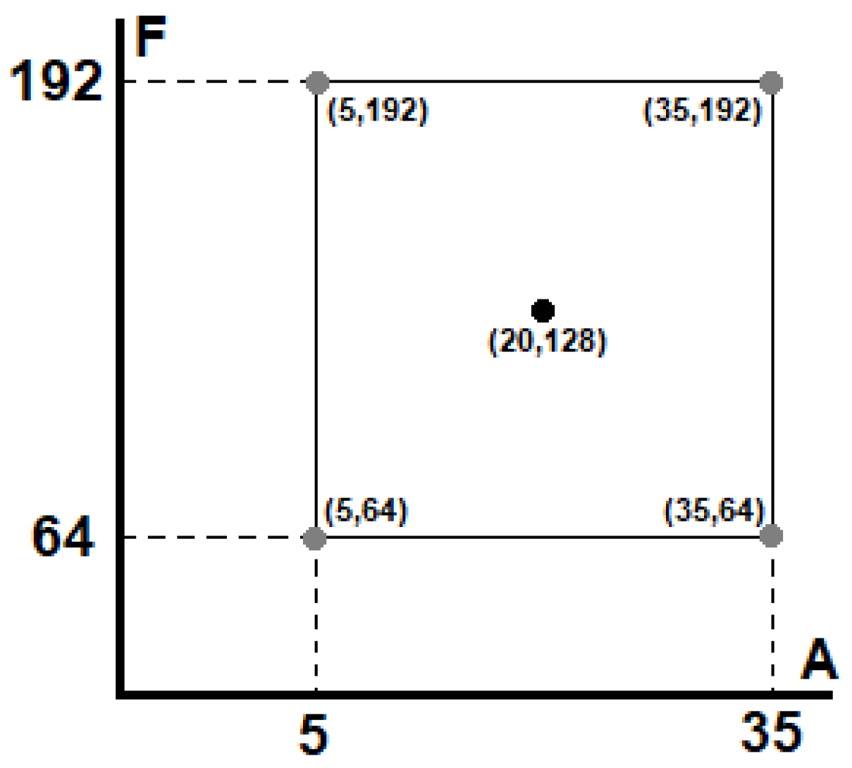
After a screening has been conducted and the two variables that mainly affect the predictive capacity of the network have been determined, a second order complete factorial experiment is performed, adding the central point to identify if there is a curvature in the model.
Figure 4 depicts this approach.
Taking advantage of the fact that the remaining factors have no impact on the prediction capacity of the model, they are adjusted to their lower value (-1) in order to reduce the computational effort and processing time. The results obtained are shown in
Table 4.
Both in the linear and quadratic models, the only significant factor that minimizes the MAE is the size of the sequence, being significant only in the linear model of the RMSE. In this manner, the transformer architecture model that optimizes the prediction of the gas outlet pressure from the electric current consumed in the motor is defined by: Sequence size (5), Head size (64), No. heads (2), FF dimension (2), No. encoder blocks (2), mlp units (64) and learning rate (0.0015).
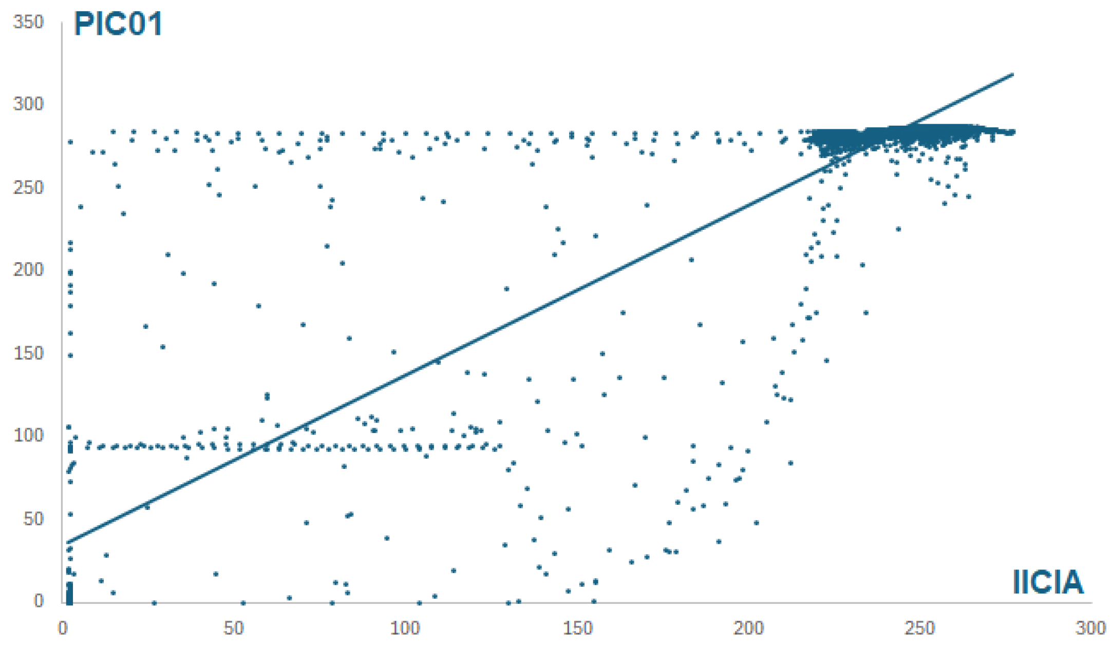
Figure 5 shows a scatter diagram between motor consumption and output pressure for the training data. Their relationship being determined by y = 1.0274x + 34.24 (R² = 0.8654). The MAE of the test data in the regression model is 18.995 compared to 7.005 obtained by the neural network. This indicates that the prediction capacity is superior to that obtained by using more basic tools.
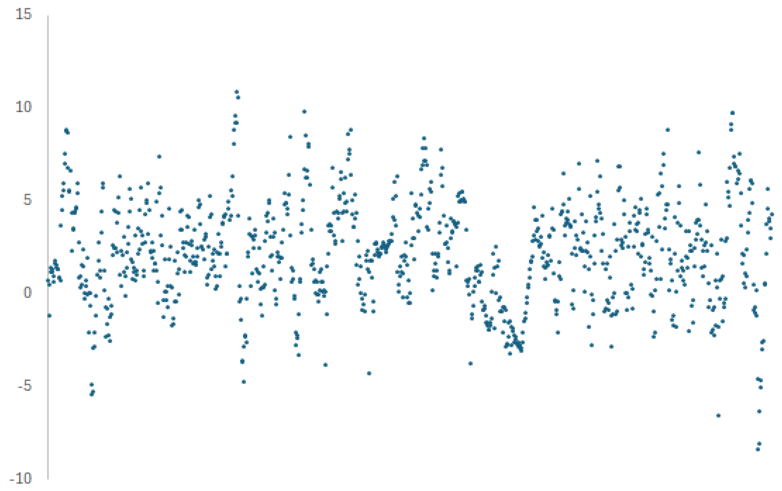
If only the last 1,000 data points of the time series are considered, the results improve since the series is more stable, which reduce the mean absolute error to 2.848. The residuals, understood as the difference between the real value and the predicted value, present a bias, since they do not have a mean of zero, but rather 2,205, as is illustrated on
Figure 6. According to [
39], biases in machine learning are primarily attributed to the nature of the data utilized and can be classified into three distinct categories: covariate shift, sample selection bias, and imbalance bias. They can be summarized as a certain feature is not uniformly covered throughout the dataset, there is no clear correlation between a value and its label, or there are few samples for certain labeled values. The residuals exhibit a normal distribution of the data, with a standard deviation of 2.744. Therefore, the estimate given by the network can be modified by adding 2.205. In this manner, the MAE is reduced to 2.147.
If a continuous reduction of prediction error is performed, an overfitting of the test data can be observed. Thus [
40] suggest that the possible causes of this overfitting could be the use of excessively complex networks, the design, and use of models with a high number of features, or the use of few training data.
6. Conclusions
Reducing unplanned stops, needless maintenance, and preventing high asset deterioration are all part of improving the sustainability of industrial equipment. Thus, predicting their behavior using neural networks may seem counterintuitive, since the utilization of more intricate neural networks does not necessarily yield superior outcomes in terms of minimizing the prediction error in time series. Therefore, technicians and managers should not rush into the generation and design of intricate models in order to obtain better predictions (less error), since, as demonstrated in this paper, simpler architectures better capture the structure of the data.
For the given time series and the defined network, the most important hyperparameter is the length of the input sequence to the network. The shorter the sequence, the lower the error. This implies that there is no autocorrelation between lag data points and that long sequences do not add relevant any information. This situation may be attributed to the fact that the control room operators manually adjust the values of the variables prior to any type of issue or critical circumstance arising. Therefore, the appearance of bias in the predicted data suggests that there is an ambiguous relationship between the compressor engine consumption and the hydrogen outlet pressure. In other words, it is not necessarily true that the lower the consumption, the lower the pressure, and vice versa.
Neural networks designed can foresee compressor activity with a relatively low prediction error, even though the operators’ behavior is not optimal for process management because it creates bias and obscures the compressor’s true behavior.
Author Contributions
S.P.: conceptualization, methodology, investigation, writing—original draft preparation, and visualization; C.G-G.: conceptualization, methodology, investigation, writing—review and supervision; M.A.S.: conceptualization, methodology, investigation, writing—review and supervision. All authors have read and agreed to the published version of the manuscript.
Acknowledgments
This paper has been produced within the scope of the doctoral activities carried out by the lead author at the International Doctorate School of the Spanish National Distance-Learning University (EIDUNED_ Escuela Internacional de Doctorado de la Universidad Nacional de Educación a Distancia). The authors are grateful for the support provided by this institution.
Conflicts of Interest
The authors declare no conflict of interest.
References
- United Nations. Transforming Our World: The 2030 Agenda for Sustainable Development. Resolution Adopted by the General Assembly on 25 September 2015, 42809, 1-13.
- Pope, J., Bond, A., Hugé, J., & Morrison-Saunders, A. Reconceptualising sustainability assessment. Environmental impact assessment review, 2017, pp. 205-215.
- Kagermann, H., Wahlster, W., & Helbig, J. Recommendations for implementing the strategic initiative Industrie 4.0. Frankfurt: Acatech-National Academy of Science and Engineering, 2013.
- Wang Z, Yan W, Oates T. Time series classification from scratch with deep neural networks: A strong baseline. In 2017 International joint conference on neural networks IEEE 2017, pp. 1578-1585.
- EN 16646. Maintenance. Maintenance within physical asset management. European Committee for Standardization. 2014.
- Baptista, M., Sankararaman, S., de Medeiros, I. P., Nascimento Jr, C., Prendinger, H., & Henriques, E. M. Forecasting fault events for predictive maintenance using data-driven techniques and ARMA modeling. Computers & Industrial Engineering, 2018, 115, 41-53.
- Francis, F., & Mohan, M. Arima model based real time trend analysis for predictive maintenance. In 2019 3rd International conference on Electronics, Communication and Aerospace Technology -ICECA. IEEE, 2019, pp. 735-739.
- Rodrigues, J. A., Farinha, J. T., Mendes, M., Mateus, R., & Cardoso, A. M. Short and long forecast to implement predictive maintenance in a pulp industry. Eksploatacja i Niezawodność, 2022, 24, 1.
- Lee, E.A. Cyber physical systems: Design challenges. In 2008 11th IEEE international symposium on object and component-oriented real-time distributed computing IEEE 2008, pp. 363-369.
- Jazdi, N. Cyber physical systems in the context of Industry 4.0. In 2014 IEEE international conference on automation, quality and testing, robotics IEEE. 2014, pp. 1-4.
- Alguliyev R, Imamverdiyev Y, Sukhostat L. Cyber-physical systems and their security issues. Computers in Industry 100. 2018, pp 212-223.
- Monostori L, Kádár B, Bauernhansl T, Kondoh S, Kumara S, Reinhart G, Sauer O, Schuh G, Sihn W, Ueda K. Cyber-physical systems in manufacturing. Cirp Annals, 2016, 65(2), pp 621-641.
- Cotrino A., Sebastián M. A., & González-Gaya C. Industry 4.0 HUB: a collaborative knowledge transfer platform for small and medium-sized enterprises. Applied Sciences, 2021, 11(12), 5548.
- Cotrino A., Sebastián M. A., & González-Gaya C. Industry 4.0 roadmap: Implementation for small and medium-sized enterprises. Applied sciences, 2020, 10(23), 8566.
- Jan B, Farman H, Khan M, Imran M, Islam IU, Ahmad A, et al. Deep learning in big data Analytics: a comparative study. Comput Electr Eng, 2019, 75, 275-87.
- Wason, R. Deep learning: evolution and expansion. Cognit Syst Res, 2018, 52, 701-8.
- Kumar U, Galar D. Maintenance in the era of industry 4.0: issues and challenges. Quality, IT and Business Operations: Modeling and Optimization, 2018, pp 231-250.
- Ghaleb, M., & Taghipour, S. Evidence-based study of the impacts of maintenance practices on asset sustainability. International Journal of Production Research, 2023, 61(24), 8719-8750.
- Kanawaday A, Sane A. Machine learning for predictive maintenance of industrial machines using IoT sensor data. In 2017 8th IEEE international conference on software engineering and service science IEEE 2017, pp 87-90.
- Zeng, A., Chen, M., Zhang, L., & Xu, Q. Are transformers effective for time series forecasting? In Proceedings of the AAAI conference on artificial intelligence, 2023, 37, 9, pp. 11121-11128.
- Wang, Y., & Zhao, Y. Multi-scale remaining useful life prediction using long short-term memory. Sustainability, 2022, 14(23), 15667.
- Abidi, M. H., Mohammed, M. K., & Alkhalefah, H. Predictive Maintenance Planning for Industry 4.0 Using Machine Learning for Sustainable Manufacturing. Sustainability, 2022, 14, 3387.
- Greener, J. G., Kandathil, S. M., Moffat, L., & Jones, D. T. A guide to machine learning for biologists. Nature Reviews Molecular Cell Biology, 2022, 23(1), 40-55.
- Murphy, K. P. Machine learning: a probabilistic perspective. MIT press, 2012.
- Zhou, L., Pan, S., Wang, J., & Vasilakos, A. V. Machine learning on big data: Opportunities and challenges. Neurocomputing, 2017, 237, 350-361.
- Li, N., Shepperd, M., & Guo, Y. A systematic review of unsupervised learning techniques for software defect prediction. Information and Software Technology, 2020, 122, 106287.
- Kaiser, L., Babaeizadeh, M., Milos, P., Osinski, B., Campbell, R. H., Czechowski, K., … & Michalewski, H. Model-based reinforcement learning for Atari. arXiv preprint, 2019, arXiv:1903.00374.
- Sultan, H. H., Salem, N. M., & Al-Atabany, W. Multi-classification of brain tumor images using deep neural network. IEEE access, 2019, 7, 69215-69225.
- Goldberg, Y. Neural network methods for natural language processing. Springer Nature, 2022.
- Ahmed, S., Nielsen, I. E., Tripathi, A., Siddiqui, S., Ramachandran, R. P., & Rasool, G. Transformers in time-series analysis: A tutorial. Circuits, Systems, and Signal Processing, 2023, 1-34.
- Haarman, M., Mulders, M., Vassiliadis, C. Predictive maintenance 4.0: Predict the unpredictable. In PwC documents, no. PwC & mainnovation, 2017, p. 31.
- Bahdanau D, Cho K, Bengio Y. Neural machine translation by jointly learning to align and translate. arXiv preprint, 2014. arXiv:1409.0473.
- Luong, M. T., Pham, H., & Manning, C. D. Effective approaches to attention-based neural machine translation. arXiv preprint 2015, arXiv:1508.04025.
- Vaswani A, Shazeer N, Parmar N, Uszkoreit J, Jones L, Gomez AN, Kaiser Ł, Polosukhin I. Attention is all you need. Advances in neural information processing systems, 2017, 30.
- LeCun, Y., Bottou, L., Bengio, Y., & Haffner, P. Gradient-based learning applied to document recognition. Proceedings of the IEEE 1998, 86(11), pp 2278-2324.
- Wang, Z., Yan, W., & Oates, T. Time series classification from scratch with deep neural networks: A strong baseline. In 2017 International joint conference on neural networks IEEE, 2017, pp. 1578-1585.
- Ioffe, S., & Szegedy, C. Batch normalization: Accelerating deep network training by reducing internal covariate shift. In International conference on machine learning, 2015, pp. 448-456.
- Zaremba, W., Sutskever, I., & Vinyals, O. Recurrent neural network regularization. arXiv preprint, 2014, arXiv:1409.2329.
- Gu, J., & Oelke, D. Understanding bias in machine learning. arXiv preprint, 2019, arXiv:1909.01866.
- Ying, X. An overview of overfitting and its solutions. In Journal of physics: Conference series. IOP Publishing, 2019, Vol. 1168, No. 2, p. 022022.
|
Disclaimer/Publisher’s Note: The statements, opinions and data contained in all publications are solely those of the individual author(s) and contributor(s) and not of MDPI and/or the editor(s). MDPI and/or the editor(s) disclaim responsibility for any injury to people or property resulting from any ideas, methods, instructions or products referred to in the content. |
© 2024 by the authors. Licensee MDPI, Basel, Switzerland. This article is an open access article distributed under the terms and conditions of the Creative Commons Attribution (CC BY) license (https://creativecommons.org/licenses/by/4.0/).
