Submitted:
01 August 2024
Posted:
02 August 2024
You are already at the latest version
Abstract
Keywords:
1. Introduction
2. Literature Review
2.1. Current Research Status of Emergency Material Distribution
2.2. Current Research Status of Vehicle-UAV Integrated Delivery Path Optimization
2.3. Current Research of Solving Methods for Routing Optimization Problem
3. Research Methodology
3.1. Modeling Ideas
3.1.1. Objective Functions
3.1.2. Constraints
4. Results and Discussions
4.1. Data Preprocessing for UAV Delivery to Customers
4.1.1. UAV Customer Clustering Processing Based on DBSCAN Algorithm
4.1.2. Dual Objective Processing in the Model
4.1.3. Artificial Bee Colony Algorithm Initialization and Neighborhood Search Strategy
4.1.5. Adaptive Probability Design for Following Bees
4.2. A Demonstrative Case
4.3. Discussions
5. Improved Artificial Bee Colony
5.1. Results Analysis
6. Conclusions and Discussions
6.1. Conclusions
6.2. Future Work
Author Contributions
Funding
Data Availability Statement
Conflicts of Interest
References
- Li, X. F. (2022). Analysis of Implementing the National Emergency System Plan for the 14th Five Year Plan [J] Labor Protection. (04): 30-32.
- Lee, M., Choi, M., Yang, T., Kim, J., Kim, J., Kwon, O., & Cho, N. (2024). A Study on the Advancement of Intelligent Military UAVs: Focusing on Reconnaissance Operations. IEEE Access.
- Fan, B., Li, Y., Zhang, R., & Fu, Q. (2020). Review on the technological development and application of UAV systems. Chinese Journal of Electronics, 29(2), 199-207. [CrossRef]
- Dorling, K., Heinrichs, J., Messier, G. G., & Magierowski, S. (2016). Vehicle routing problems for UAV delivery. IEEE Transactions on Systems, Man, and Cybernetics: Systems, 47(1), 70-85.
- Scott, J. E., & Scott, C. H. (2019). Models for UAV delivery of medications and other healthcare items. Unmanned aerial vehicles: Breakthroughs in research and practice, 376-392.
- Maharana, A., Amutorine, M., Sengeh, M. D., & Nsoesie, E. O. (2021). COVID-19 and beyond: Use of digital technology for pandemic response in Africa. Scientific African, 14, e01041. [CrossRef]
- Sudbury, A. W., & Hutchinson, E. B. (2016). A cost analysis of amazon prime air (UAV delivery). Journal for Economic Educators, 16(1), 1-12.
- Pressroom, U. P. S. (2020). UPS flight forward, CVS To Launch residential UAV delivery service in Florida retirement community to assist in coronavirus response. UPS Pressroom, 27.
- Bamburry, D. (2015). UAVs: Designed for product delivery. Design Management Review, 26(1), 40-48.
- Ahmed, J. U., Islam, Q. T., Islam, S., Ahmed, A., & Mim, K. P. (2022). Last-Mile UAV Delivery: Is Wing's Business Model Sustainable?. SAGE Publications: SAGE Business Cases Originals.
- Demuyakor, J. (2020). Ghana go digital Agenda: The impact of zipline UAV technology on digital emergency health delivery in Ghana. Humanities, 8(1), 242-253.
- Reddy, T. B. S., Teja, P. H., Teja, R. P., & Praneeth, T. (2019). Adaptive Autonomous Technology in Unmanned Aerial Vehicles for Parcel Delivery. [CrossRef]
- Liu, Y., Liu, Z., Shi, J., Wu, G., & Pedrycz, W. (2020). Two-echelon routing problem for parcel delivery by cooperated truck and UAV. IEEE Transactions on Systems, Man, and Cybernetics: Systems, 51(12), 7450-7465.
- Jung, H., & Kim, J. (2022). UAV scheduling model for delivering small parcels to remote islands considering wind direction and speed. Computers & Industrial Engineering, 163, 107784.
- Hu, Z. J. (2018). Research on the dispatch and transportation optimization of emergency materials for urban flood disasters [D] Shenyang: Shenyang University of Technology.
- Deng Xiuqin, Ni Weihong, etc. Research on emergency logistics and material support system based on blockchain under the COVID-19 [J] Logistics Technology and Applications, 2020, 25 (10): 176-179.
- Julie, Cao Jie, Gu Jun. A Study on the Dynamic Allocation of Emergency Supplies for Fair Relief of Trauma in Disaster Victims [J] Systems Engineering Theory and Practice, 2020, 40 (9): 2427-2437.
- Qin J., Xu J. L. (2023). Research on Optimization of Emergency Support Service Network for Livelihood Materials under the Background of Sudden Infectious Disease Epidemic [J]. Journal of Railway Science and Engineering, 20 (6): 1-11.
- Yu, G. H. (2012). Research on the Occupying Path Problem of Unconventional Disaster Emergency Logistics Based on Complex Networks [D] Guangzhou: South China University of Technology.
- Wu, T., He, L., & Yu, H. (2022). Online traveling salesman problem with time cost and non-zealous server. Journal of Combinatorial Optimization, 1-24. [CrossRef]
- Su B., Geng X. Y., (2022). Research on the unpredictable emergency material distribution path selection for service requests at demand points [J] Chinese Management Science, 30 (11): 1-10.
- Wohlsen, M. (2014). The Next Big Thing You Missed: Amazon’s Delivery UAVs Could Work—They Just Need Trucks. Wired: Business, Jun, 10.
- Yurek, E. E., & Ozmutlu, H. C. (2018). A decomposition-based iterative optimization algorithm for traveling salesman problem with UAV. Transportation Research Part C: Emerging Technologies, 91, 249-262.
- de Freitas, J. C., & Penna, P. H. V. (2018). A randomized variable neighborhood descent heuristic to solve the flying sidekick traveling salesman problem. Electronic Notes in Discrete Mathematics, 66, 95-102.
- Sacramento, D., Pisinger, D., & Ropke, S. (2019). An adaptive large neighborhood search metaheuristic for the vehicle routing problem with UAVs. Transportation Research Part C: Emerging Technologies, 102, 289-315.
- Cavani, S., Iori, M., & Roberti, R. (2021). Exact methods for the traveling salesman problem with multiple UAVs. Transportation Research Part C: Emerging Technologies, 130, 103280.
- Murray, C. C., & Raj, R. (2020). The multiple flying sidekicks traveling salesman problem: Parcel delivery with multiple UAVs. Transportation Research Part C: Emerging Technologies, 110, 368-398.
- Liu, W. S., Li, W., Zhou, Q. (2021). Optimization model and algorithm for "UAV-vehicle" delivery path[J]. Department of Transportation Unified Engineering and Information, 21(6): 176-186.
- Leibo, Y. A. N. G., & Jun, Z. H. O. U. (2023). Research on Distribution Path Problem of Truck Combined with UAV in Restricted Area. Journal of Computer Engineering & Applications, 59(12).
- Tamke, F., & Buscher, U. (2023). The vehicle routing problem with UAVs and UAV speed selection. Computers & Operations Research, 152, 106112.
- Moshref-Javadi, M., Hemmati, A., & Winkenbach, M. (2020). A truck and UAVs model for last-mile delivery: A mathematical model and heuristic approach. Applied Mathematical Modelling, 80, 290-318.
- Lin, M., Lyu, J. Y., Gao, J. J., & Li, L. Y. (2020). Model and hybrid algorithm of integrated distribution system with multiple UAVs and a truck. Scientific Programming, 2020, 1-16.
- Zhang, R., Dou, L., Xin, B., Chen, C., Deng, F., & Chen, J. (2023). A review on the truck and UAV cooperative delivery problem. Unmanned Systems, 1-25.
- Boyd, S., & Mattingley, J. (2007). Branch and bound methods. Notes for EE364b, Stanford University, 2006, 07.
- Yufeng, L., & Jun, L. (2012). Dynamic programming heuristic algorithm for solving time-varying vehicle scheduling problems [J]. Systems Engineering Theory and Practice, 32, 1712-1718.
- Ou, W., Jiao L (2011). A dynamic planning algorithm for the vehicle path problem under Ping contingency[J]. Computer Simulation, 28(08):354-358.
- Lin, S., & Kernighan, B. W. (1973). An effective heuristic algorithm for the traveling-salesman problem. Operations research, 21(2), 498-516. [CrossRef]
- Solomon, M. M. (1987). Algorithms for the vehicle routing and scheduling problems with time window constraints. Operations research, 35(2), 254-265. [CrossRef]
- Lin, S. (1965). Computer solutions of the traveling salesman problem. Bell System Technical Journal, 44(10), 2245-2269. [CrossRef]
- Vigo, D. (1996). A heuristic algorithm for the asymmetric capacitated vehicle routing problem. European Journal of Operational Research, 89(1), 108-126.
- Sun, X. J., Jie K. W. (2018). An improved ant colony algorithm for solving dynamic vehicle routing problems with time windows [J] Journal of Dalian University of Technology, 58 (05): 539-546.
- Wei, M., Jin W. Z. (2010). Discrete particle swarm optimization algorithm for solving vehicle routing problems [J] Computer Science, 37 (04): 187-191.
- Qian, J. B., Zhang, J. X., Yao, D. W. (2022). A Particle Swarm Optimization Algorithm Based on Improved Inertial Weights [J] Computer and Digital Engineering, 50 (08): 1667-1670.
- Feng Tao. Enacting UAV flight management law-clarifying flight management authorities [N]. Legal Daily.2022-9-20.
- Huang J, Hu Yueli et al. Implementation of combined navigation system on a quadcopter UAV[J]. Electronic Technology Application, 2015, 41(05):167- 170.
- Zhou Jiajun, Wan Ran. Problems and Countermeasures Analysis of Urban Logistics UAV Delivery[J]. Information System Engineering.2021, 5(09):142-144. Path Optimization Research on Cooperative Distribution of Emergency Supplies by Vehicles and UAVs.
- Zhou Lang. Optimization study of rural e-commerce logistics distribution "delivery truck + UAV" path [D]. Hubei:Wuhan University of Technology, 2017.
- Kirk, J. Fixed Endpoints Open Traveling Salesman Problem - Genetic Algorithm [J]. Acta Universitatis Carolinae. medica monographia, 1973, 56(2):7-20.
- Hassanalian, M., & Abdelkefi, A. (2017). Classifications, applications, and design challenges of UAVs: A review. Progress in Aerospace sciences, 91, 99-131.
- Yang, Su. Research and Application of Vehicle Path Problem Based on Improved Artificial Bee Colony Algorithm [D]. Chongqing:Chongqing University. 2018.
- Li Jiahui. Research on Path Optimization Method of Urban Logistics and Distribution Vehicles [D]. Jilin:Changchun University of Science and Technology, 2021.
- Osman I, H. Metastrategy simulated annealing and tabu search algorithms for the vehicle routing problem [J]. Annals Ops Res, 1993, 41(4):421-451.
- Xiong Chuanming. Research on Scheduling and Path Planning Algorithm Based on Cooperative Delivery by UAV and Truck [D]. Hubei:Huazhong Science University of Technology, 2018.
- Ester, M., Kriegel, H. P., Sander, J., & Xu, X. (1996, August). Density-based spatial clustering of applications with noise. In Int. Conf. knowledge discovery and data mining (Vol. 240, No. 6).
- Zhang, J. H. Application of simulated annealing ant colony algorithm in optimal path selection[J]. Journal of Huaihua College, 2022. 41(05) :68-75.
- Metropolis N, Rosenbluth A W, Rosenbluth M N. Equation of State Calculations by Fast Computing Machines [J]. Journal of Chemical Physics, 2004, 21(6):1087-1092. [51]Kirkpatrick S, Vecchi M P. Optimization by simulated annealing [M]. Readings in computer vision: issues, problems, principles, and paradigms. Morgan Kaufmann Publishers Inc. 1987:339-348.
- Metropolis, N., Rosenbluth, A. W., Rosenbluth, M. N., Teller, A. H., & Teller, E. (1953). Equation of state calculations by fast computing machines. The journal of chemical physics, 21(6), 1087-1092. [CrossRef]
- Kirkpatrick, S., Gelatt Jr, C. D., & Vecchi, M. P. (1983). Optimization by simulated annealing. science, 220(4598), 671-680.
- Rubinstein, R. Y., & Kroese, D. P. (2016). Simulation and the Monte Carlo method. John Wiley & Sons.
- Ryan E, P. A universal adaptive stabilizer for a class of nonlinear systems [J]. Systems & Control Letters, 1991, 16(3):209-218.
- Kang, L.-S. Non-numerical Parallel Algorithm-Simulated Annealing Algorithm [M]. Beijing:Science Press, 1994.
- XU Xiaoping, ZHU Qiqiu. Improved simulated annealing algorithm for solving TSP[J]. Computer System Applications, 2015. 24(12):152-156.
- WANG Yu, SHIN Hyun-kyung et al. An artificial bee colony algorithm for solving the shortest path problem in transportation networks[J]. Journal of Jilin University, 2021, 59(5): 1144-1150.
- Jiang, M.Y., Yuan D.F.. Artificial bee colony algorithm and its application [M]. Beijing:Science Press, 2014.

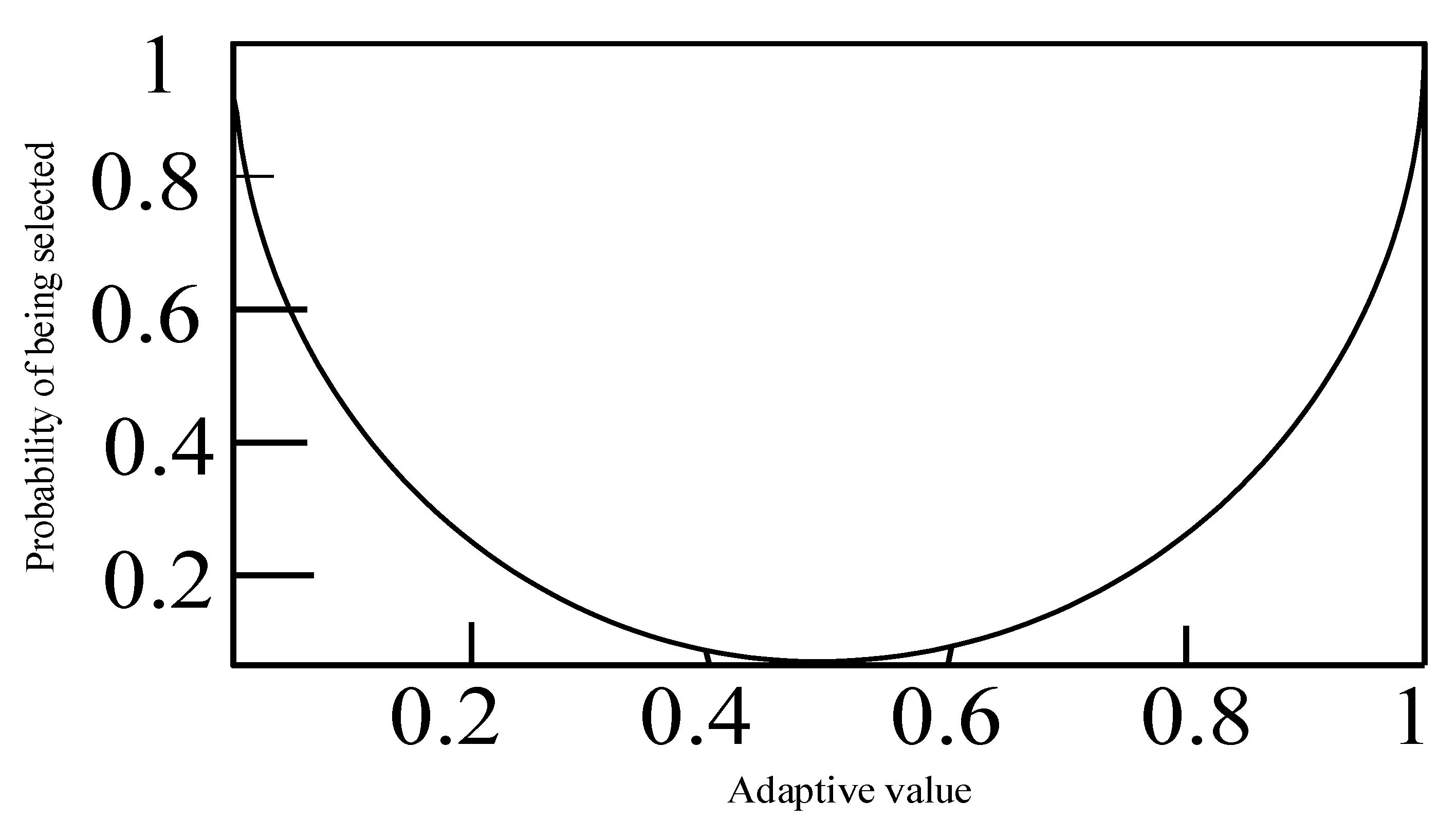
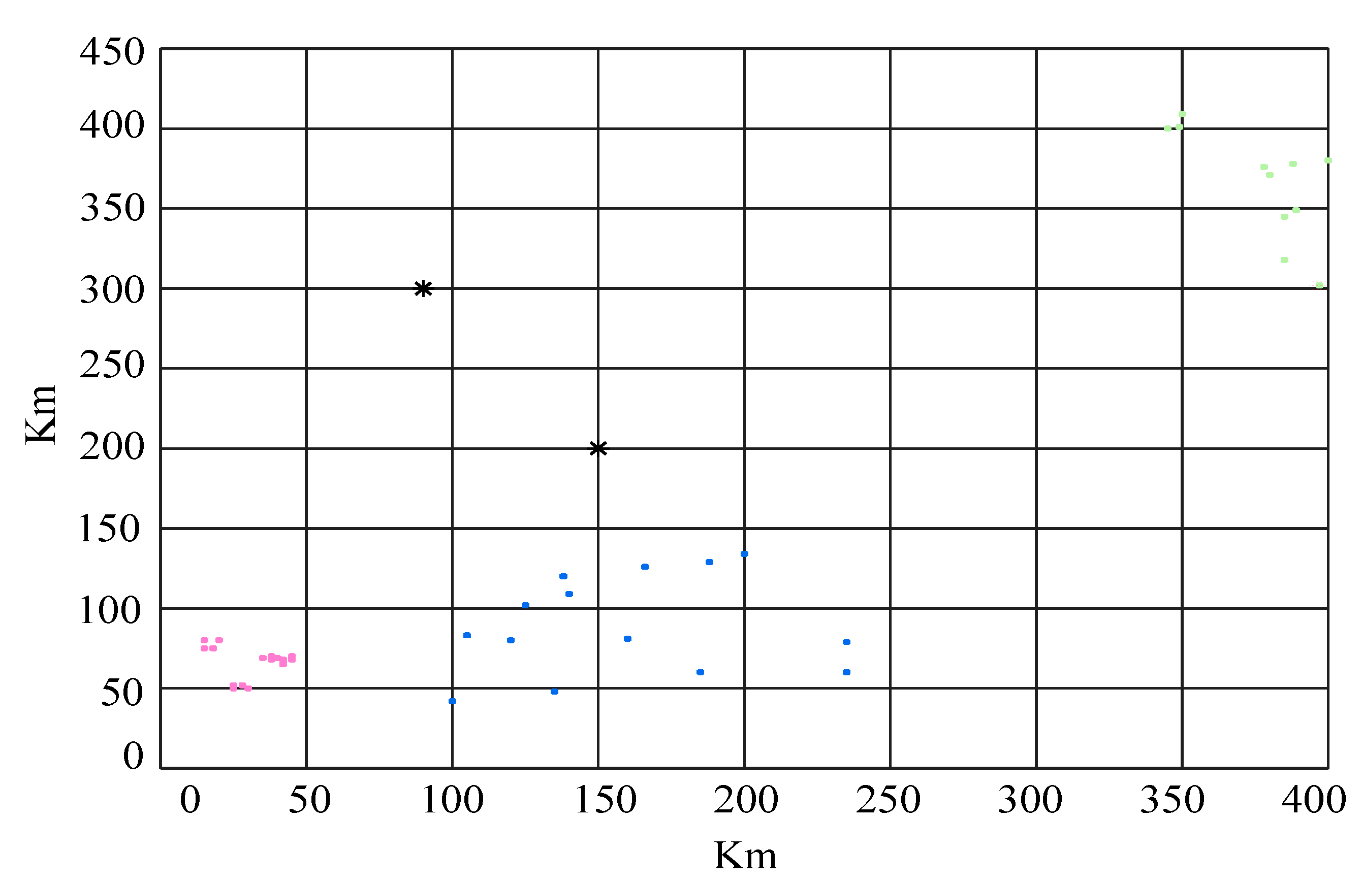
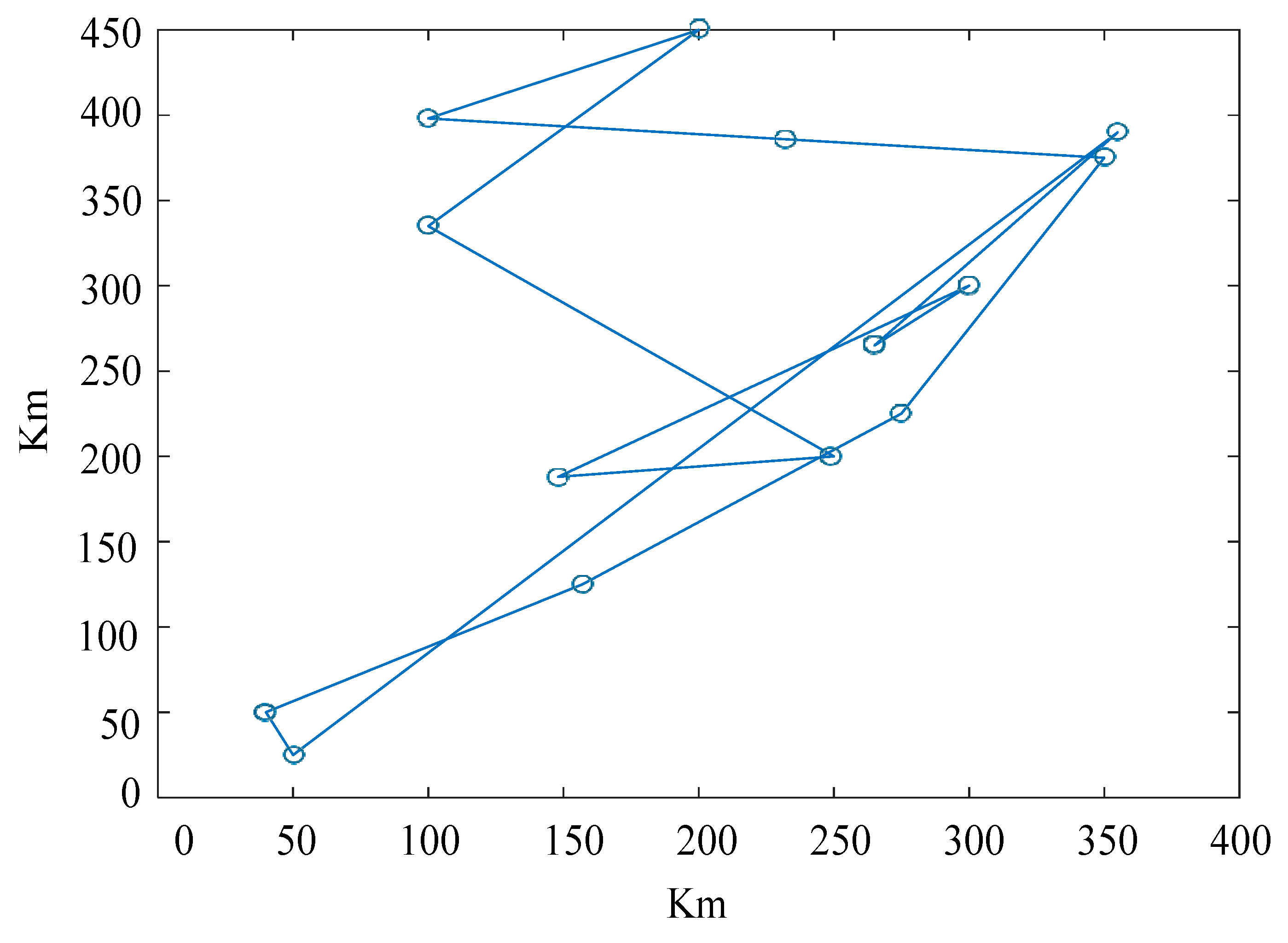
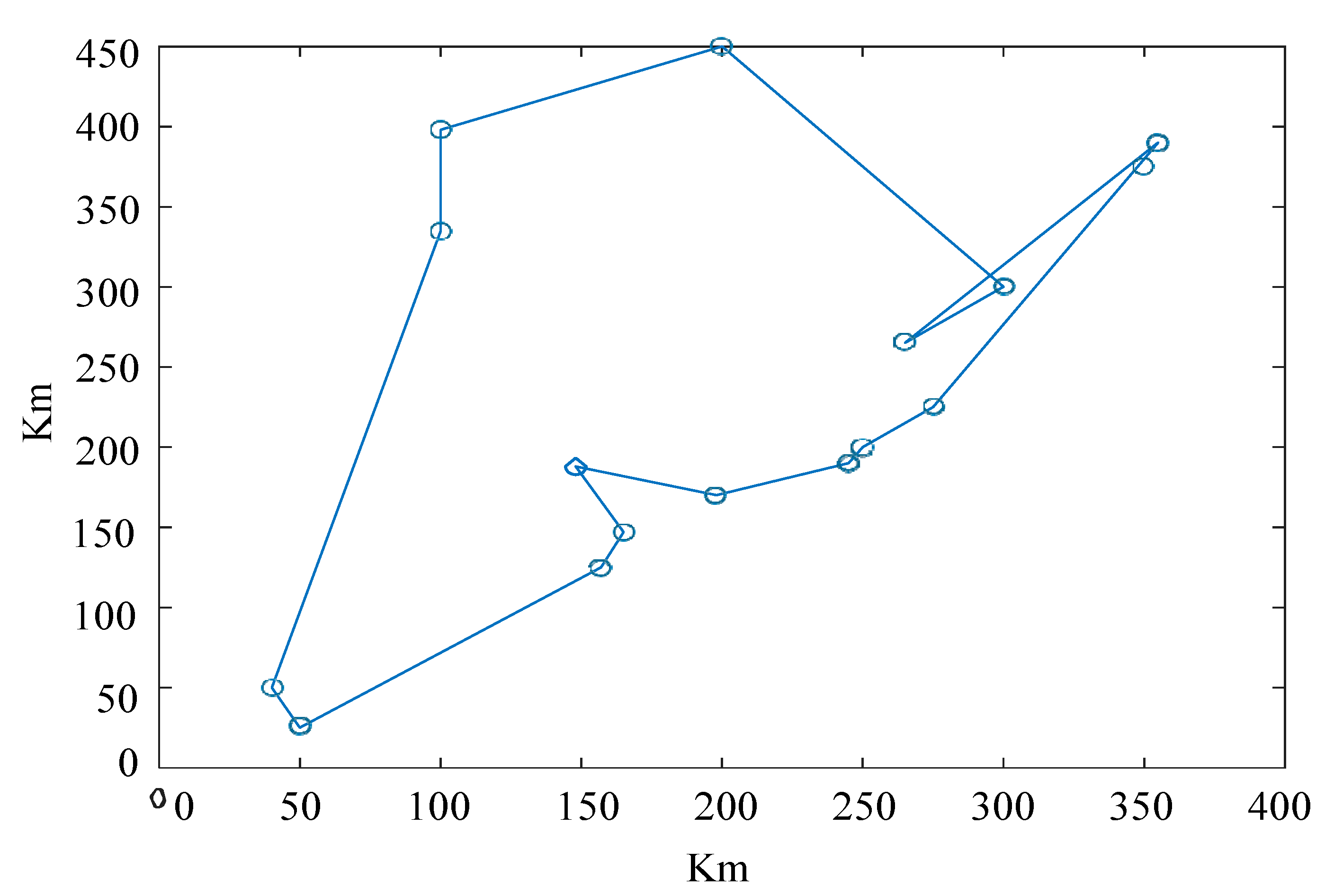
| Basic parameters | Basic parameters |
| Number of vehicles used/vehicle 1 | Number of available UAVs 4 |
| Customer point service time/min 20 | Maximum capacity of UAV/kg 200 |
| Bee colonies 40 | The farthest flying distance of UAVs/km 50 |
| Exchange probability 0.15 | UAV violation of capacity constraint penalty coe fficient 10 |
| Insertion probability 0.35 | Average vehicle speed/km/h 80 |
| Reverse order probability 0.5 | UAV flying speed/km/h 150 |
| Delivery point | X-axis coordinates | Y-axis coordinates | Demand (kg) | Earliest expected arrival time (min) | Latest expected arrival time (min) | |
| Vehicles can get to passengers |
0 | 50 | 25 | 0 | 0 | 1000 |
| 1 | 157 | 125 | 40 | 70 | 140 | |
| 2 | 355 | 390 | 70 | 180 | 720 | |
| 3 | 100 | 335 | 60 | 300 | 500 | |
| 4 | 148 | 188 | 20 | 100 | 360 | |
|
Vehicles can get to passengers |
5 | 40 | 50 | 30 | 80 | 180 |
| 6 | 165 | 147 | 50 | 90 | 200 | |
| 7 | 350 | 375 | 90 | 300 | 500 | |
| 8 | 300 | 300 | 30 | 260 | 560 | |
| 9 | 275 | 225 | 60 | 190 | 700 | |
| 10 | 250 | 200 | 20 | 200 | 480 | |
| 11 | 245 | 190 | 35 | 290 | 750 | |
| 12 | 198 | 170 | 40 | 190 | 640 | |
| 13 | 265 | 265 | 50 | 240 | 590 | |
| 14 | 200 | 450 | 70 | 220 | 800 | |
| 15 | 250 | 400 | 90 | 560 | 950 | |
| 16 | 100 | 398 | 65 | 630 | 900 | |
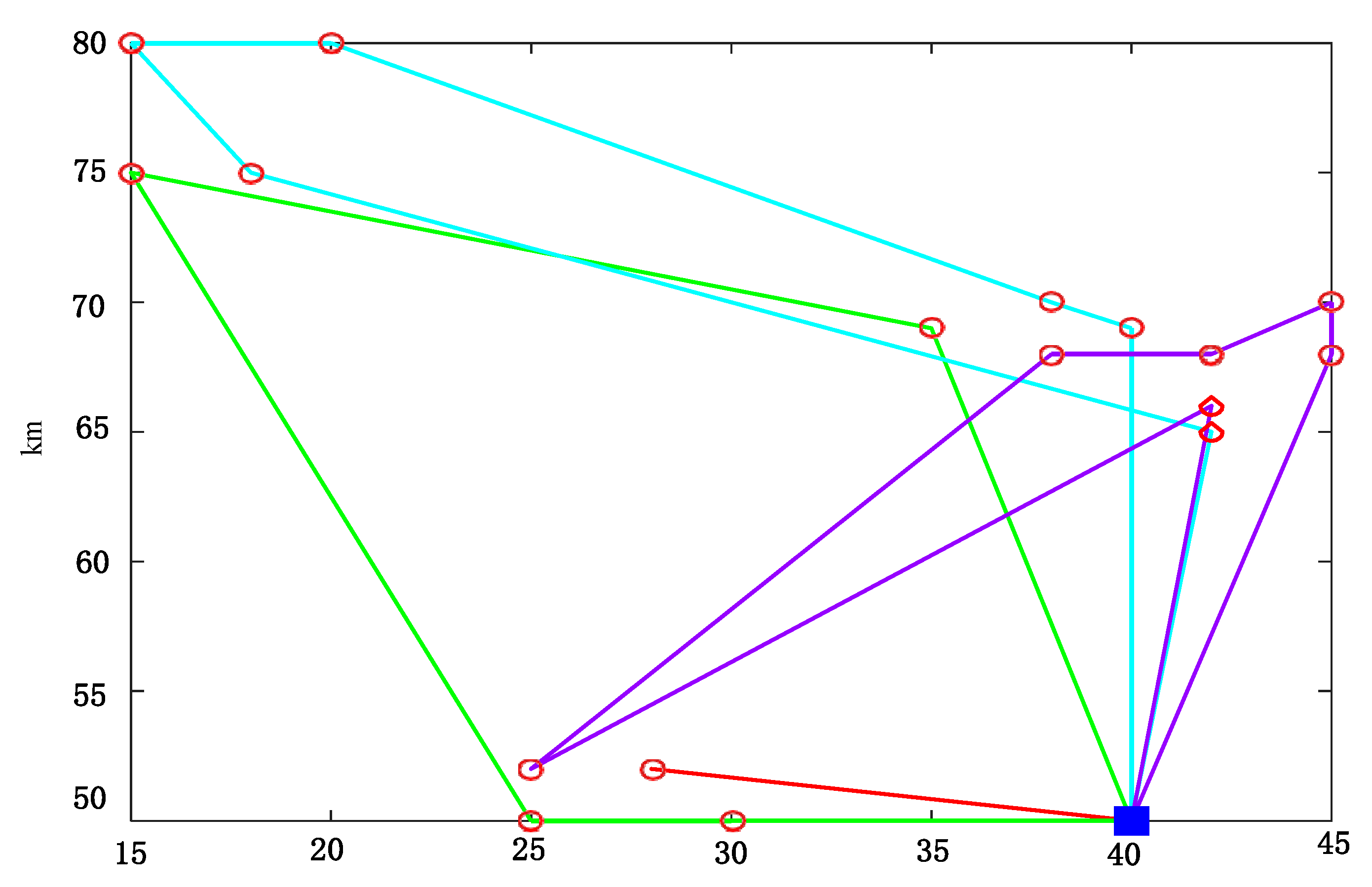
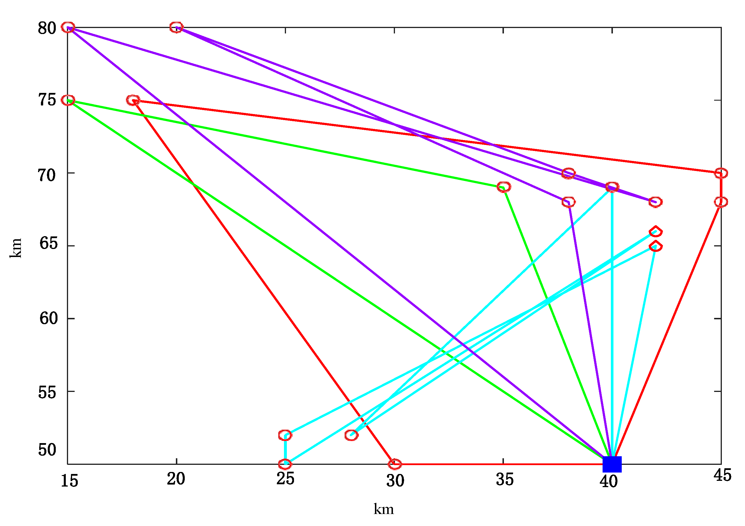
| Delivery UAVs | 1 | 45 | 68 | 10 | 912 | 967 |
| 2 | 45 | 70 | 30 | 825 | 870 | |
| 3 | 42 | 66 | 10 | 65 | 146 | |
| 4 | 42 | 68 | 10 | 727 | 782 | |
| 5 | 42 | 65 | 10 | 15 | 67 | |
| 6 | 40 | 69 | 20 | 621 | 702 | |
| 7 | 38 | 68 | 20 | 255 | 324 | |
| 8 | 38 | 70 | 10 | 534 | 605 | |
| 9 | 35 | 69 | 10 | 448 | 505 | |
| 10 | 20 | 80 | 40 | 384 | 429 | |
| 11 | 18 | 75 | 20 | 99 | 148 | |
| 12 | 15 | 75 | 20 | 179 | 254 | |
| 13 | 15 | 80 | 10 | 278 | 345 | |
| 14 | 30 | 50 | 10 | 10 | 73 | |
| 15 | 28 | 52 | 20 | 812 | 883 | |
| 16 | 25 | 50 | 10 | 65 | 144 | |
| 17 | 25 | 52 | 40 | 169 | 224 | |
| 18 | 135 | 48 | 10 | 812 | 867 | |
| 19 | 185 | 60 | 30 | 525 | 570 | |
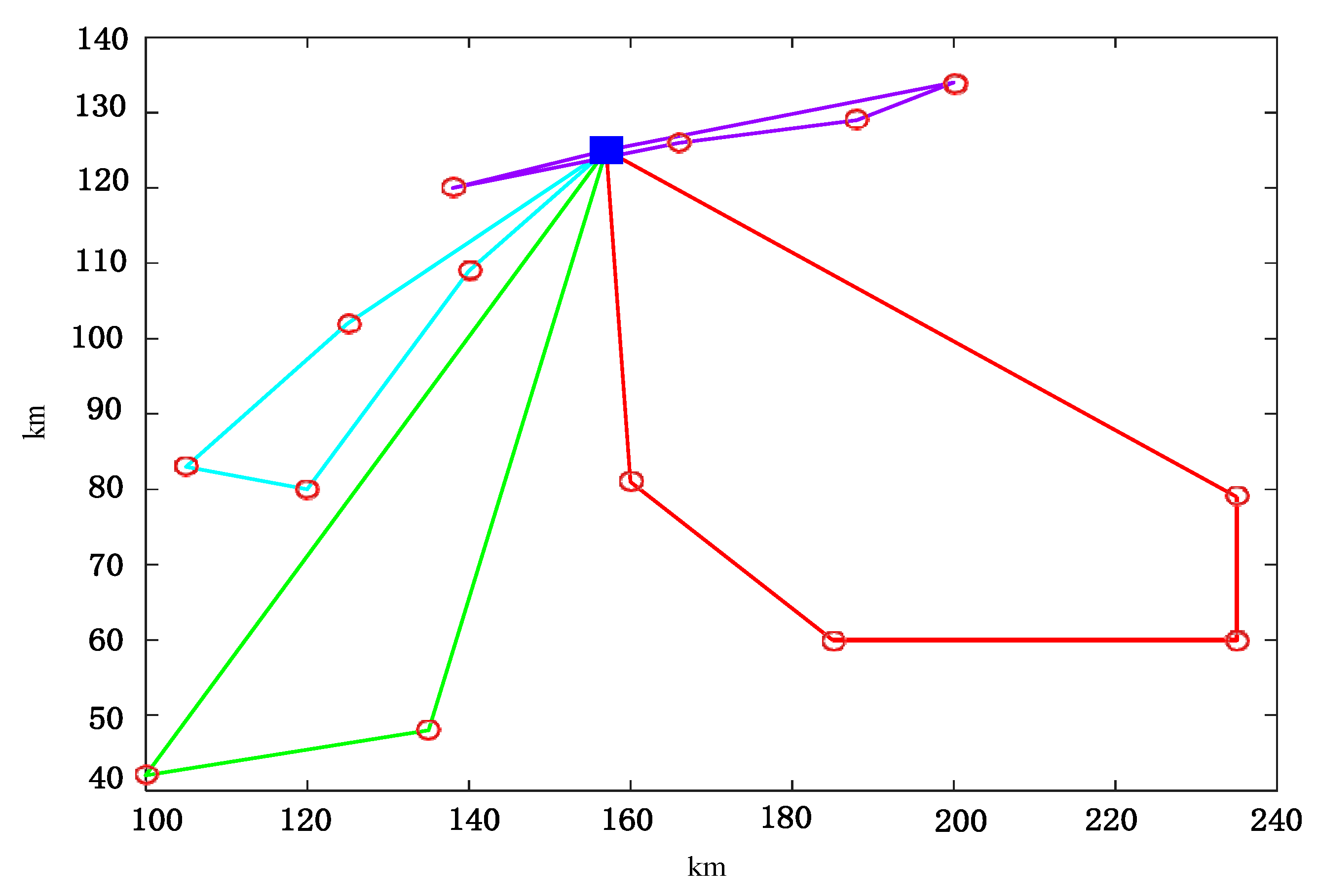
| 20 | 166 | 126 | 10 | 85 | 126 | |
| 21 | 120 | 80 | 10 | 327 | 442 | |
| 22 | 140 | 109 | 20 | 531 | 602 | |
| 23 | 200 | 134 | 10 | 534 | 605 | |
| 24 | 235 | 60 | 10 | 348 | 405 | |
| 25 | 188 | 129 | 40 | 284 | 329 | |
| 26 | 125 | 102 | 20 | 179 | 254 | |
| 27 | 105 | 83 | 10 | 278 | 345 | |
| 28 | 235 | 79 | 10 | 40 | 93 | |
| 29 | 160 | 81 | 20 | 712 | 803 | |
| 30 | 138 | 120 | 10 | 35 | 104 | |
| 31 | 100 | 42 | 40 | 119 | 164 | |
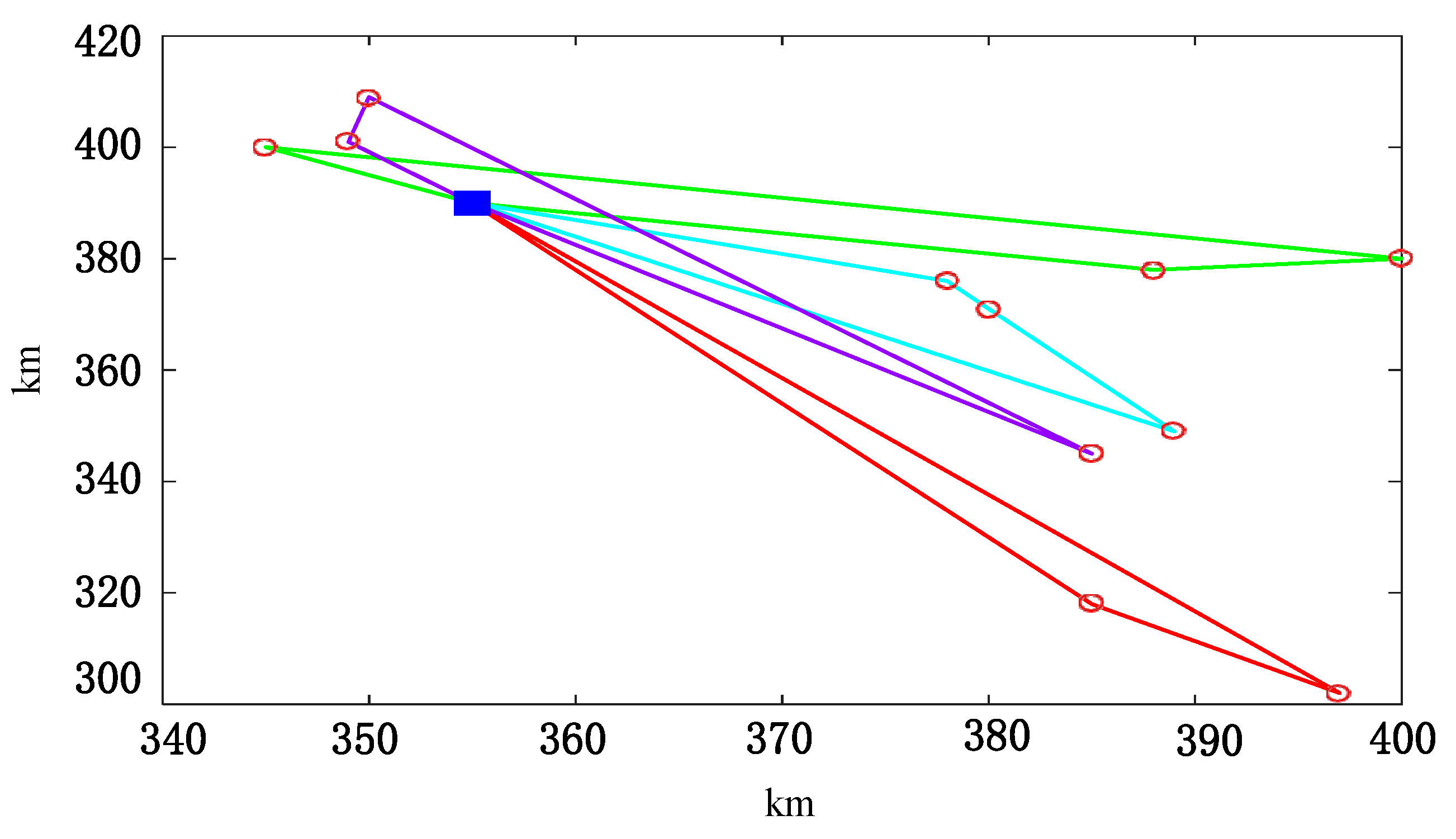
| 32 | 385 | 318 | 40 | 812 | 867 | |
| 33 | 380 | 371 | 30 | 525 | 570 | |
| 34 | 385 | 345 | 10 | 612 | 657 | |
| 35 | 397 | 302 | 40 | 525 | 570 | |
| 36 | 345 | 400 | 20 | 225 | 246 | |
| 37 | 350 | 409 | 50 | 387 | 432 | |
| 38 | 388 | 378 | 10 | 415 | 467 | |
| 39 | 389 | 349 | 20 | 301 | 382 | |
| 40 | 400 | 380 | 30 | 185 | 224 | |
| 41 | 378 | 376 | 50 | 428 | 505 | |
| 42 | 349 | 401 | 30 | 254 | 289 | |
| 43 | 90 | 300 | 20 | 554 | 689 | |
| 44 | 150 | 200 | 10 | 855 | 867 |
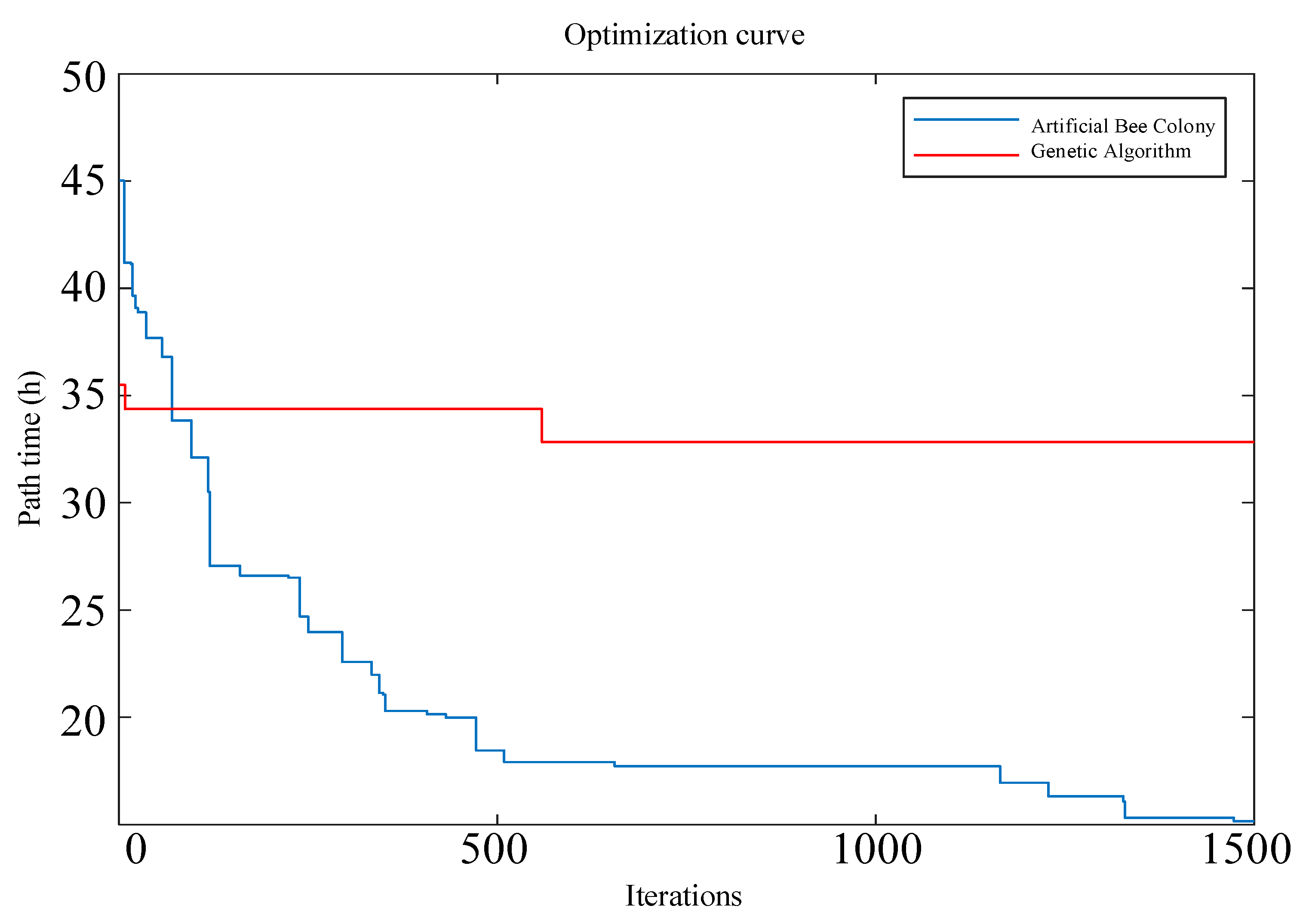
| Genetic algorithm | Artificial Bee Colony (ABC) | |
| Iterations | 1500 | 1500 |
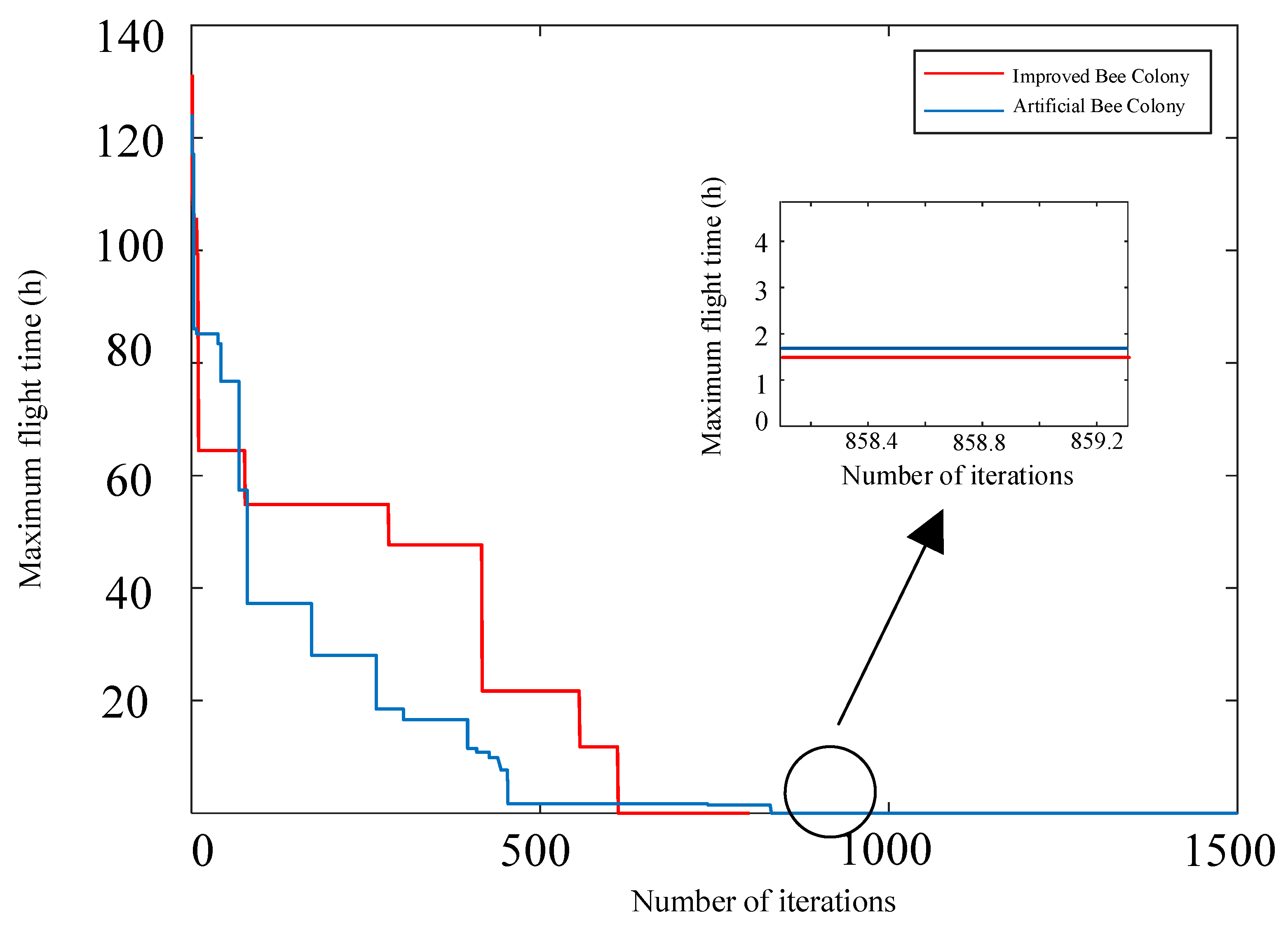
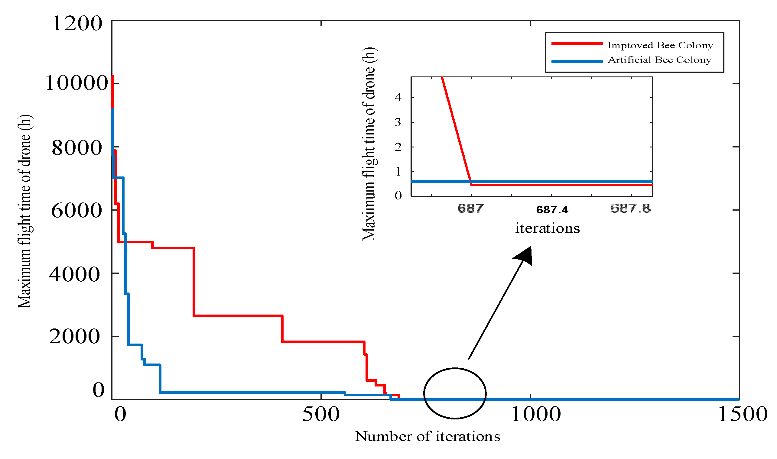
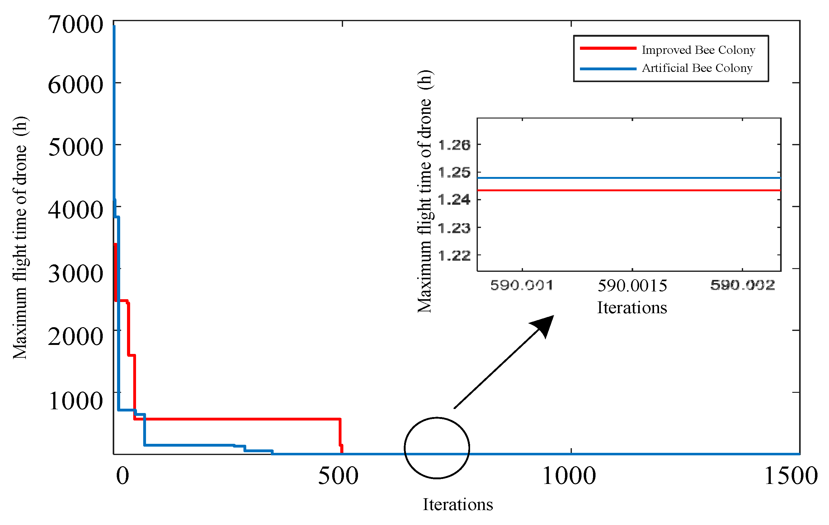
| Total delivery time of vehicles and UAVs/h | 58 | 21.8 |
| Algorithm average running time/s | 24 | 14 |
| Algorithm name | Path sequence | Path time/h | Iterations | Algorithm time/s |
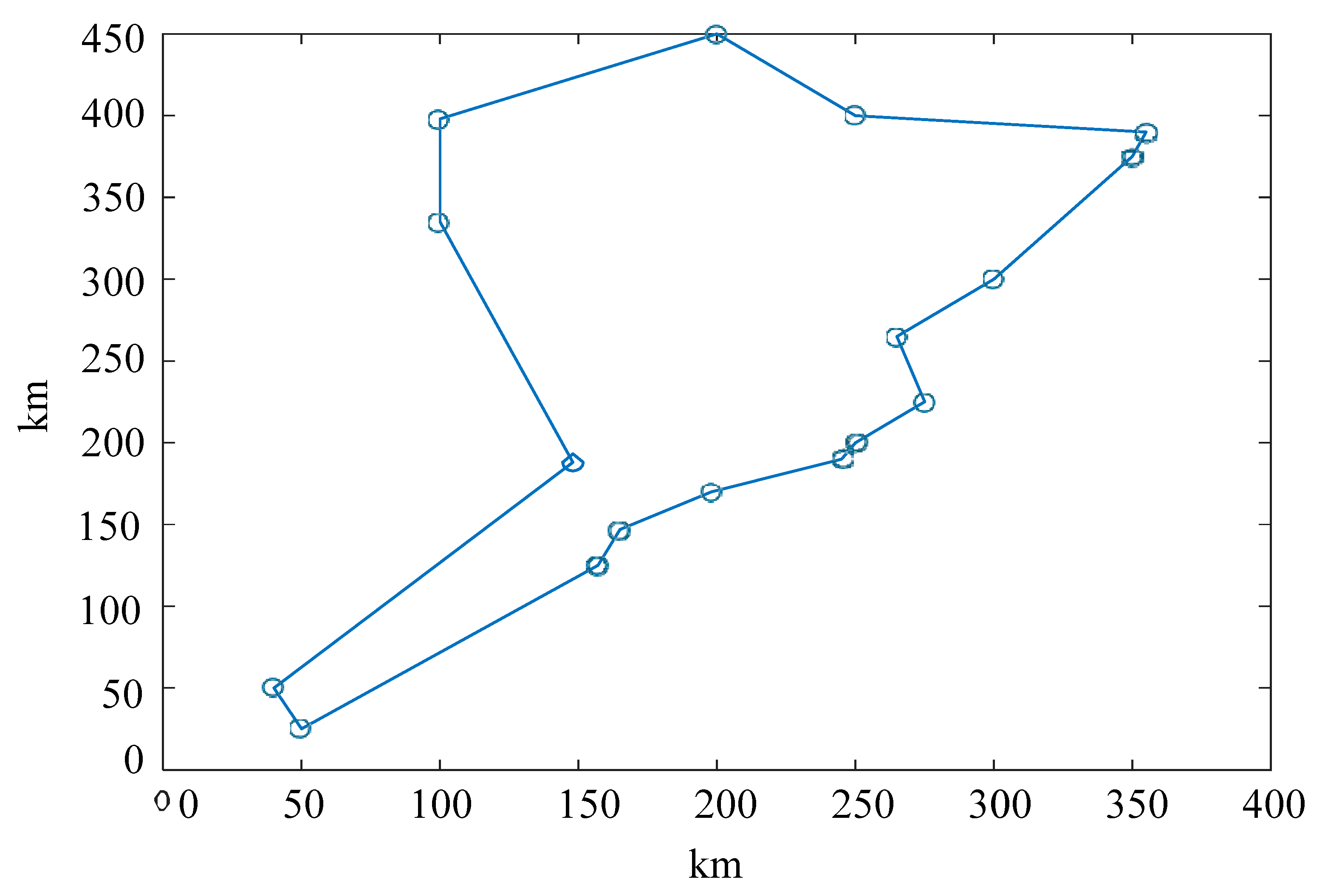
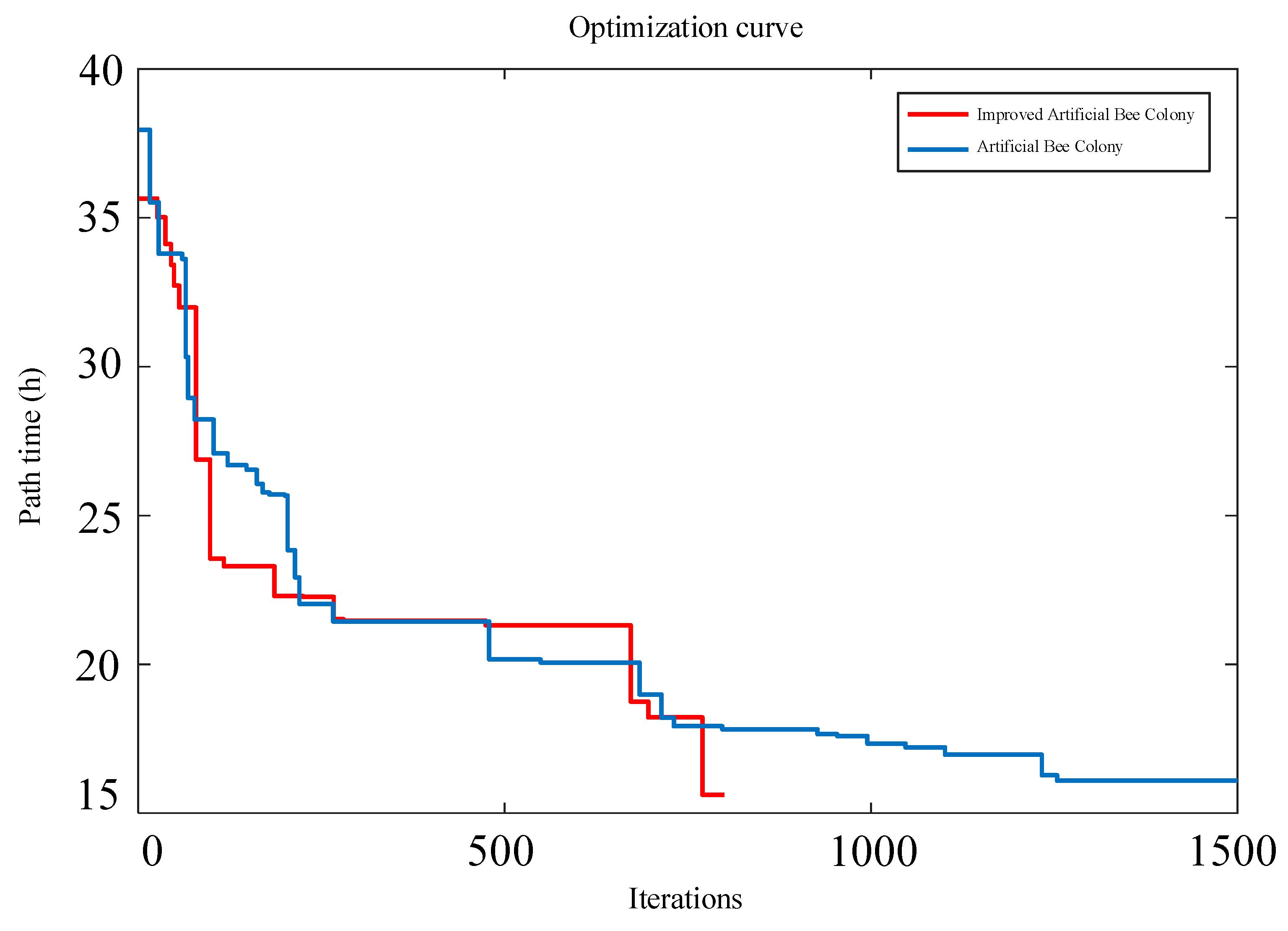
| Artificial bee colony | 0 1 6 12 13 8 11 10 9 2 7 15 14 16 3 4 5 | 17.8631 | 1500 | 10.5 |
| Improved bee colony | 0 5 4 3 16 14 15 2 7 8 13 9 10 11 12 6 1 | 15.1601 | 800 | 6.3 |
| Index | Artificial bee colony algorithm | Improving the bee colony algorithm |
| Vehicle-UAV total path time/h | 21.8 | 18.2 |
| Iterations | 1500 | 800 |
| Algorithm average running time/s | 14 | 7.5 |
Disclaimer/Publisher’s Note: The statements, opinions and data contained in all publications are solely those of the individual author(s) and contributor(s) and not of MDPI and/or the editor(s). MDPI and/or the editor(s) disclaim responsibility for any injury to people or property resulting from any ideas, methods, instructions or products referred to in the content. |
© 2024 by the authors. Licensee MDPI, Basel, Switzerland. This article is an open access article distributed under the terms and conditions of the Creative Commons Attribution (CC BY) license (http://creativecommons.org/licenses/by/4.0/).


