Designing the Chemical Composition of Steel with Required Hardenability Using Computational Methods

This paper introduces an innovative approach that enables automated and precise prediction of the steel's chemical composition based on the desired Jominy curve. The microstructure, and in fact the presence of martensite, is decisive for the hardness of the steel, so the study considered the occurrence of this phase at particular distances from the quenched-end of the Jominy sample. Steels for quenching and tempering and case hardening were investigated. With representative collected dataset of hardness values from quenched-end of Jominy specimen, microstructure and chemical composition of steels, the complex regression model was made using supervised artificial neural networks. The balance between cost and required hardenability can be achieved through optimizing the chemical composition of steel. This model of designing steel with required hardenability can be of great benefit in the mechanical engineering and manufacturing industry. The model is verified experimentally.

Keywords:

Subject: Engineering - Mechanical Engineering

1. Introduction

The selection of steel for the specific machine parts, tools or constructions is preceded by the definition of the required properties. The required properties of steels, such as hardenability, are achieved by a specific chemical composition and manufacturing process. For machine parts and tools during material production process it would be very beneficial if according to the required hardenability chemical composition of steel is known.

Hardenability is defined as the ability of ferrous alloys to acquire hardness after austenitization and quenching. This includes the ability to reach the highest possible hardness and hardness distribution within a cross section [1]. The maximum hardness of heat-treated steel depends primarily on the carbon content. Alloying elements have little effect on the maximum hardness, but they significantly affect the depth to which this maximum hardness can be developed. Thus, one of the first decisions to be made is what carbon content is necessary to obtain the desired hardness. The next step is to determine what alloy content will give the proper hardening response in the section size involved [2].

Jominy and Boegehold developed the end-quench hardenability test that characterizes the hardenability of a steel from a single specimen in the year 1938 [3]. It is still used worldwide and known as Jominy test and is part of many standards such as EN ISO 642: 1999, ASTM A255 and JIS G 0561 [4,5,6]. The result of Jominy test is the Jominy curve, which shows the measured hardness values at different distances from the quenched-end. Chemical composition of steel, as mentioned, has significant influence on the hardenability and thus numerous attempts have been made to characterize the hardenability from its chemical composition. An accurate model to calculate the hardenability (Jominy curve) in an early stage of the steel production could result in control of hardenability of the final product. Grossmann characterized hardenability by defining ideal critical diameter as the largest diameter of a cylindrical specimen which transforms into at least 50% of martensite when quenched with an infinitely large cooling rate at the surface [7]. In his later work, Grossmann proposed multiplying coefficients for alloying elements for calculation of the critical diameter [8]. Numerous studies followed trying to characterize the hardenability from its chemical composition [9,10,11,12,13,14,15,16,17,18].

Nevertheless, the relationship between the chemical composition of steel and the resulting values obtained after the Jominy end-quench test, and via versa, cannot be defined, precise enough, by any mathematical function. More complex regression analysis is necessary. Developments in computers and software have positioned artificial neural networks at the forefront in technical science in general, including material science [19,20,21,22,23,24].

Deep learning is a powerful tool for finding patterns in multi-dimensional data. Deep learning, as a subset of machine learning, uses algorithms such a computer can learn from empirical dataset by modelling nonlinear relationships between the material properties and influencing factors [25]. Artificial neural networks (ANNs) are widely used in modeling steel and metal alloy issue due to their efficiency in handling regression tasks. ANNs are characterized by their ability to learn from labeled dataset and are, therefore, well suited for supervised learning applications. The creation of representative dataset is crucial for development of an effective model based on artificial neural networks [26,27].

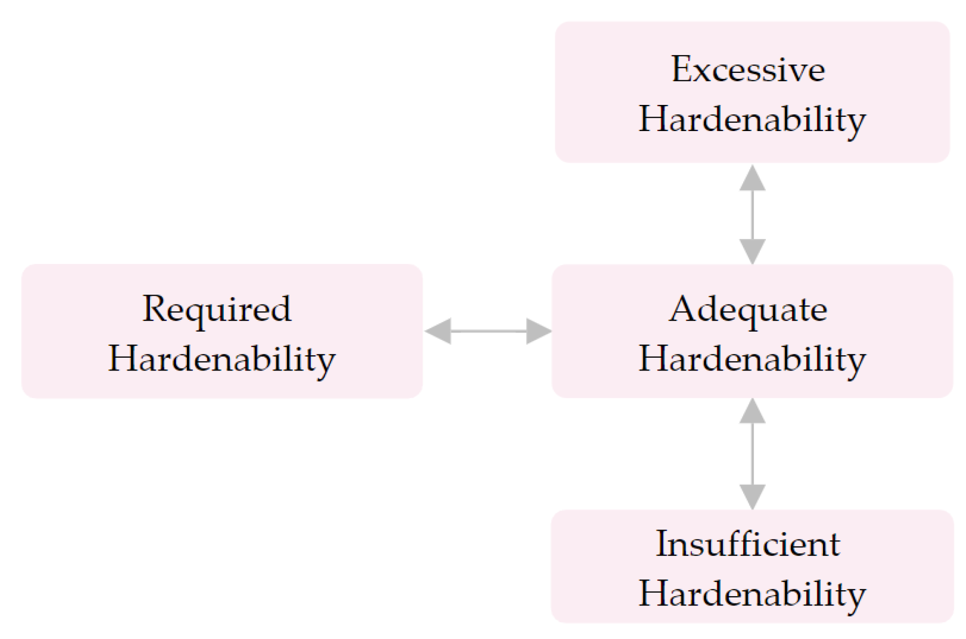
Designing the chemical composition of the steel having the required properties is the crucial task from the manufacturing point of view. Knowing the required hardenability for machine parts or tools enables designing the steel with optimal chemical composition. Such a steel will have adequate, for particular application, hardenability. Quenching and tempering of steels with insufficient hardenability, regarding its application, does not provide appropriate hardness in deeper layers and can cause functional problems. Excessive hardenability indicates usage of surplus of alloying elements and thus increasing the cost (Figure 1).

The content of alloying elements should not be higher than necessary for ensuring adequate hardenability.

In this paper an innovative approach is introduced that enables automated and precise prediction of the steel’s chemical composition based on the Jominy curve respecting microstructure at different distances from the quenched-end of Jominy specimen. Steels for quenching and tempering and case hardening were investigated. It is known that during the Jominy test, areas closer to the quenched-end are cooled faster. The result is that different microstructures are achieved at different distances from quenched-end of Jominy specimen. Steels with different chemical compositions can achieve the same microstructure (e.g. 99.9% martensite) but due to the different chemical composition (primarily carbon content) hardness values will be different [1,28]. It implies that hardness values are the result of microstructure as well as chemical composition. Considering minimization of possible errors in the input data regarding microstructure, the presence of martensite was considered. The limit is set at 50% of martensite in the microstructure. Hardness is dependent primarily on carbon content and values of hardnesses are known for different carbon content and different ratio of martensite in the microstructure [29,30]. Some authors successfully use following relation to calculate hardness with 50% of martensite in the microstructure regarding achieved maximum hardness [31,32]:

HRC_50%M = 0.73 ∙ HRC_max

(1)

The research included supervised learning of artificial neural networks so that the dataset was structured in such a way that between the predictors (hardnesses in Rockwell hardness scale C – HRC and microstructure, at specific distances from quenched-end of Jominy specimen) and responses (chemical compositions of 7 alloying elements, renumerate alloying elements) excellent relations were established. Through collecting data, modeling and optimizing regression models, the optimal artificial neural network model for designing chemical composition of steel is established.

2. Materials and Methods

2.1. Analysis of Dataset

In this research, steels for quenching and tempering and case hardening were investigated, from standards EN 10083-2, EN 10083-3, EN 10084 and similar [33,34,35]. Dataset consisted of Jominy curves, presented as the consecutive hardness values at 13 distances from the quenched-end of Jominy specimen and wt% content of alloying elements C, Si, Mn, Cr, Ni, Mo and Cu. It was assumed that the heat treatment of steel for the collected data is made under standard conditions that confirm to ASTM standard [5]. The grain size according to ASTM scale is 7. The dataset contains data of hardnesses (Rockwell hardness scale C - HRC) at distances of 1.5, 3, 5, 7, 9, 11, 13, 15, 20, 25, 30, 40 and 50 mm from quenched-end of Jominy specimen (Table 1).

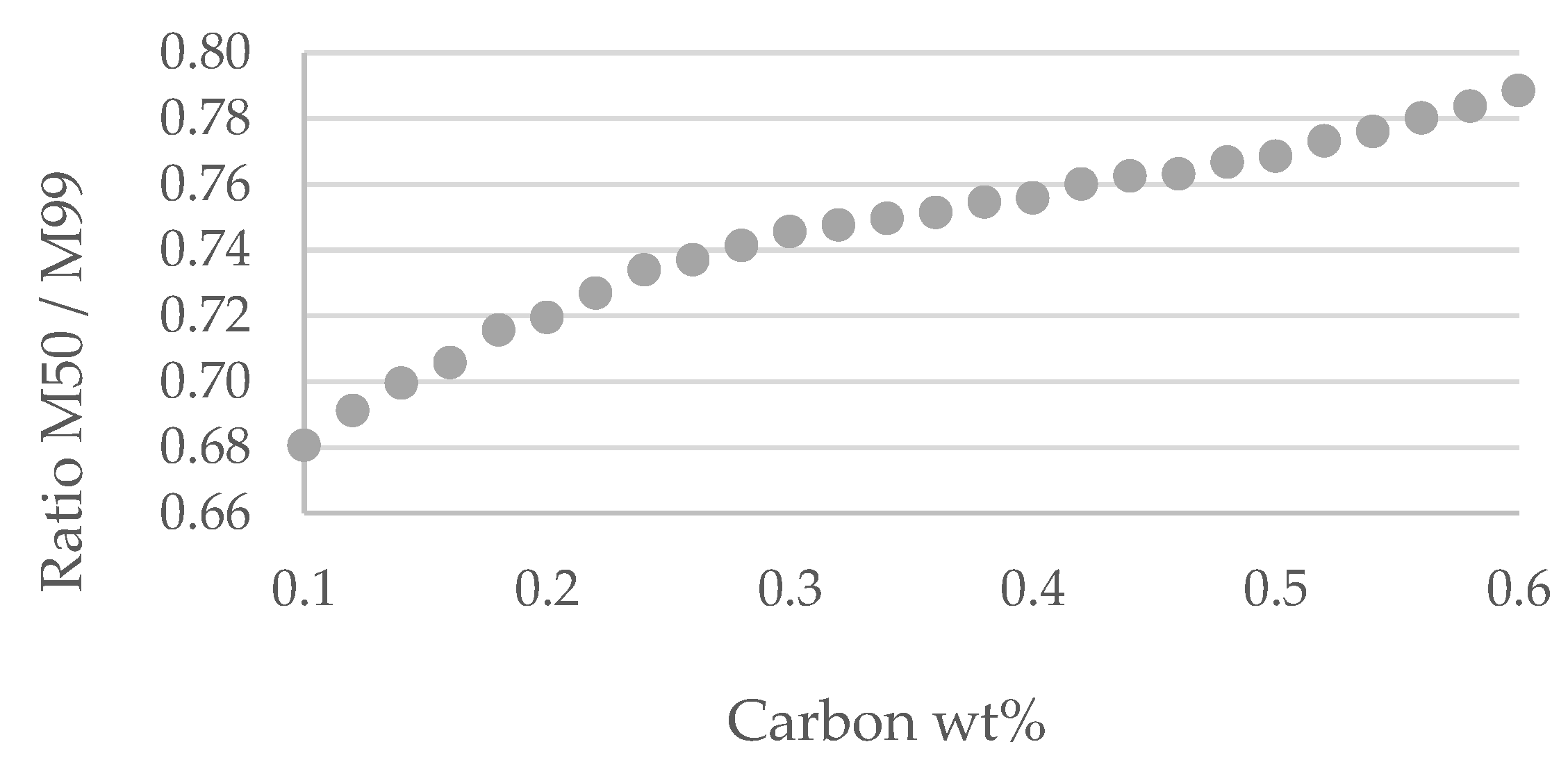
Dataset also contains information on the percentage of mass concentration of the seven alloying elements, namely C, Mn, Si, Cr, Ni, Mo and Cu. Complete homogeneity of the steel is not realistic to expect. Small deviation in homogeneity can significantly affect the microstructure distribution along the Jominy specimen. The presence of martensite was considered. The limit is set at 50% of martensite in the structure. Ratio of hardness of steel with 50% martensite in the microstructure and 99% of martensite in the microstructure for different carbon content is shown in Figure 2 [29].

For calculating the hardness value with 50% martensite (HRC_50%M), according to maximum hardness, HRC_max it is used following relation:

HRC_50%M = k ∙ HRC_max

(2)

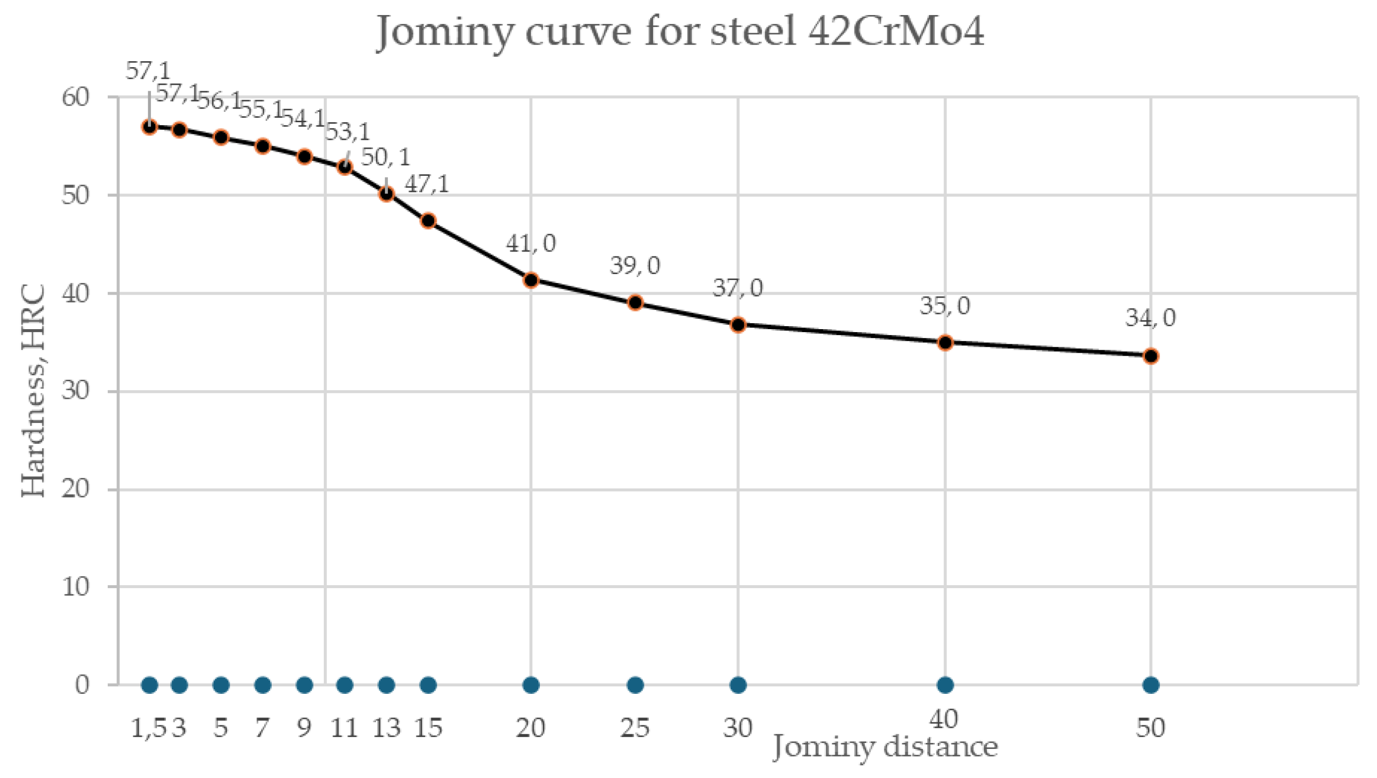
Where k is function of carbon wt%. For the distances on Jominy specimen with values of hardness greater than k ∙ HRC_max, value 1 is assign (more than 50% of martensite is presented in the microstructure). For the hardnesses lower than k ∙ HRC_max, value 0 is assign (less than 50% of martensite is presented in the microstructure). The explained procedure was performed on 470 different steels. Example of predictors for steel 42CrMo4 is shown in Table 2 and in Figure 3.

Response for the same steel is shown in Table 3.

The dataset is divided into two different subsets: a training set, which is used to determine the model parameters, and a separate test dataset (validation set). The training set is used for model parameterization, while the validation was used as an independent dataset for evaluating the model’s performance. Data partitions are done in MATLAB, using the cvpartition function. A typical application of this function is holdout validation, where the dataset is partitioned into a training set and a test set. It generates a random, non-stratified partition for holdout validation on a dataset. The proportion of observations assigned to the test set is set to 5%, while the remaining data form the training set [36].

The training dataset must be a representative sample of the data. The Kolmogorov-Smirnov (KS) test is used to evaluate the goodness of fit of the training and test dataset [37]. It checks whether the distribution of the training and test sets vary significantly. Results of Kolmogorov-Smirnov test are presented in Table 4 and Table 5.

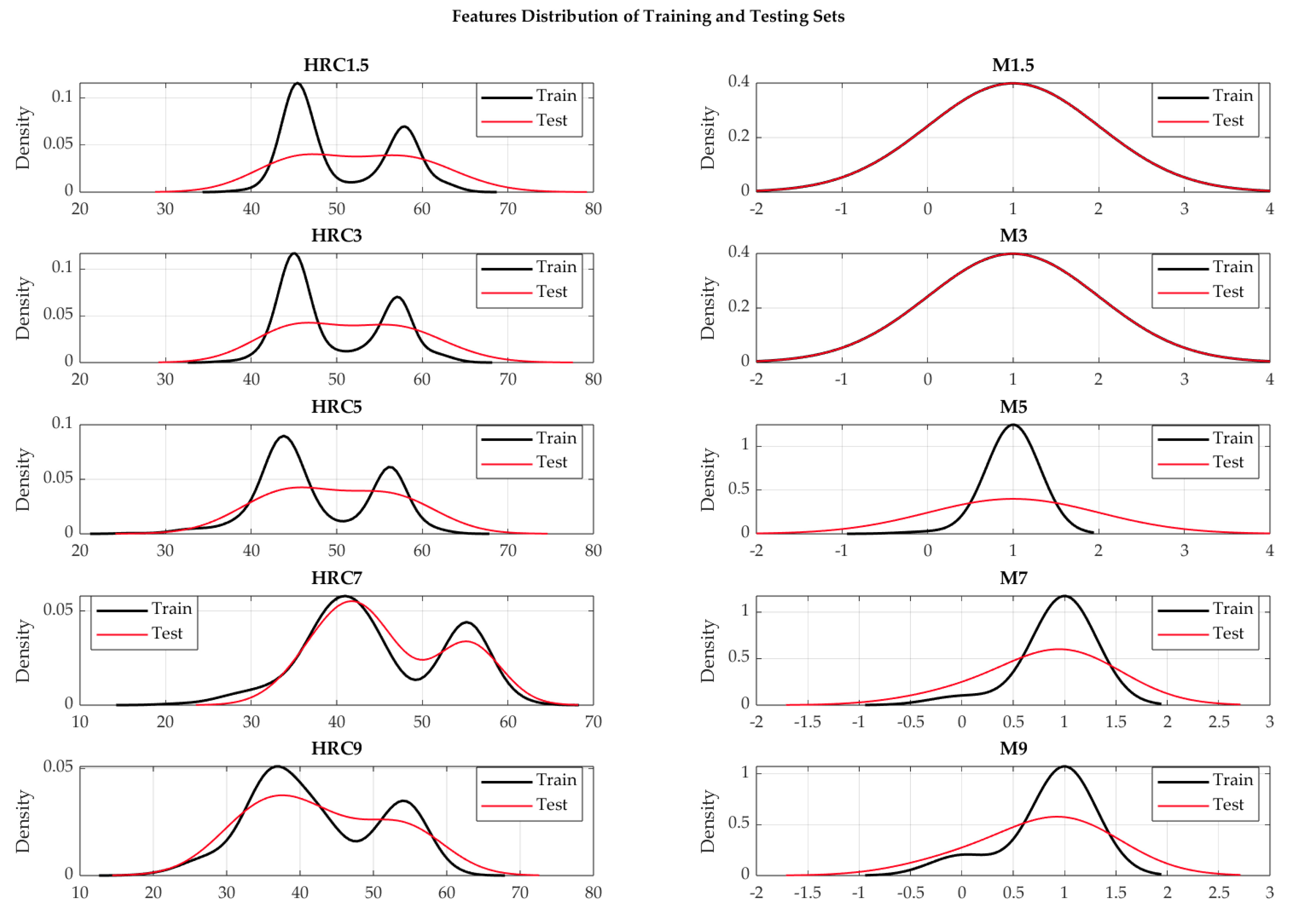
We conducted Kolmogorov-Smirnov (KS) tests for each feature at a 5% significance level to assess the similarity of feature distributions between the training and test datasets. The KS test values were calculated for the features of hardness (HRC) and microstructure at specific distances from quenched-end of Jominy specimen. The obtained KS test values are between 0.09 and 0.167 for hardness and between 0 and 0.161 for microstructure. In addition, p-values were calculated for each test, in range from 0.57 and 0.99 (hardness) and 0.96 and 1 (microstructure), indicating no substantial evidence to reject the null hypothesis of similarity between the distributions. These results that model is likely to generalize well to the unsee test dataset (Figure 4).

2.2. Experimental Setup

For regression, Machine Learning and Deep Learning Toolbox from MATLAB R2023b is used. To train neural network regression models Regression Learner App is used. For protecting overfitting, 10-fold cross-validation during the training is used. Training and test phase of model development are done for each of seven alloying elements separately. Training is done by using five deferent architectures of artificial neural networks: ‘trilayered’, ‘bilayered’, ‘narrow’, ‘medium’ and ‘wide’ neural network as well as optimized neural network. The architectures of neural networks are as follow:

trilayered [10, 10, 10], with ReLU activation function;
bilayered [10, 10], with ReLU activation function;
narrow [10], with ReLU activation function;
medium [25], with ReLU activation function;
wide [100], with ReLU activation function.

The architecture and activation function of Optimized neural networks vary.

The model with the smallest test root mean square error (RMSE) is evaluated as the best model because low RMSE can ensure that the selected model generalizes well to a new dataset. In addition to RMSE, mean square error (MSE), mean absolute error (MAE), and coefficient of determination (R²) are used to evaluate the model during the test performance analysis.

3. Results

In order to select the best-performing model for prediction chemical composition of steel, this paragraph offers a thorough overview of model evaluation and selection, performance analysis and training. The training was done separately for each chemical element. Thus, all the neural networks have input layer with 26 nodes (13 hardnesses at distances of 1.5, 3, 5, 7, 9, 11, 13, 15, 20, 25, 30, 40 and 50 mm from quenched-end of Jominy specimen and 13 values that indicate presence of martensite, higher or lower than 50%) and output layer with 1 node (chemical element).

3.1. Experimental Results Analysis

3.1.1. Experimental Result Analysis for Carbon

The artificial neural network models are placed in the table according to the lowest RMSE (Table 6).

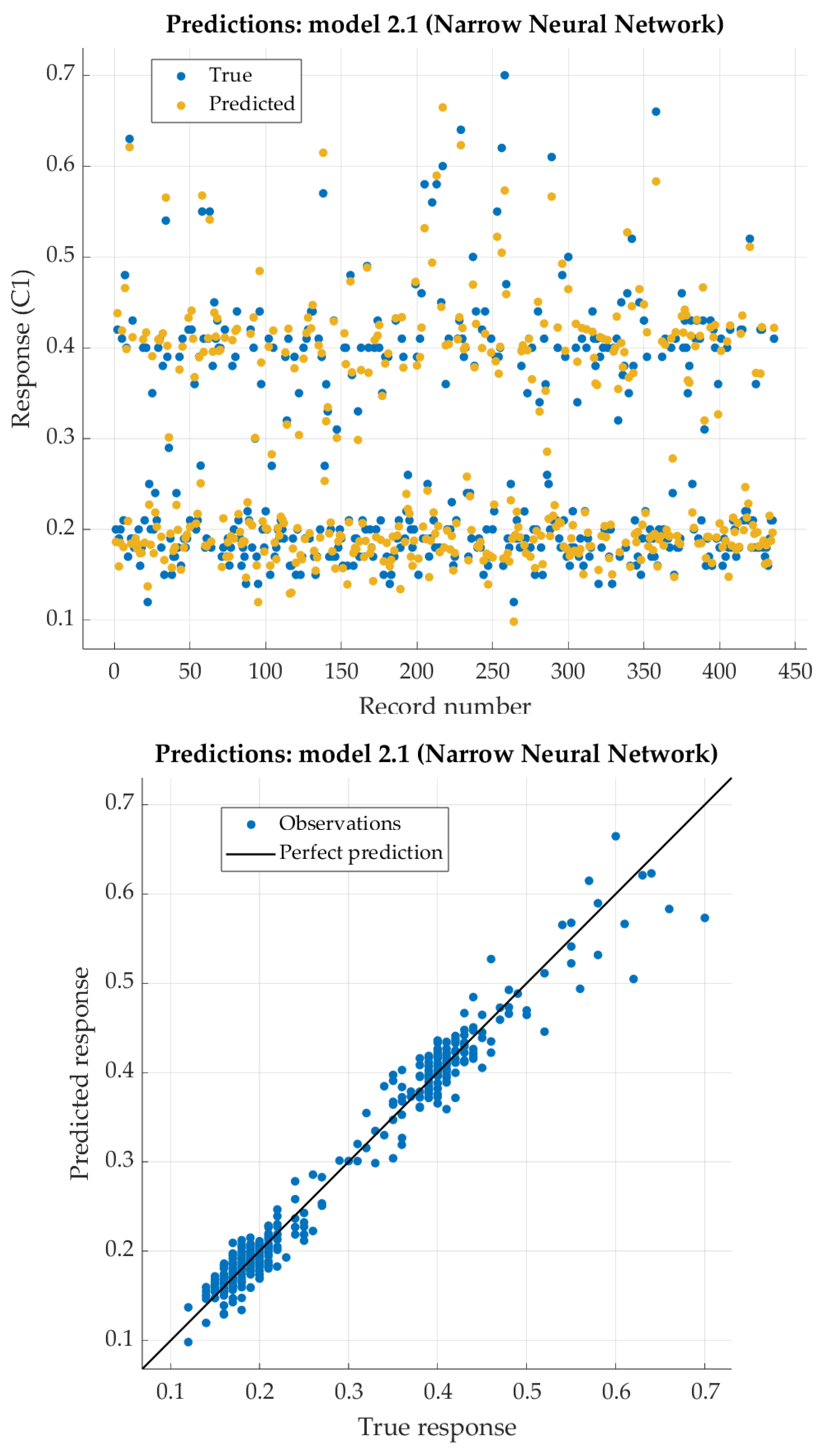
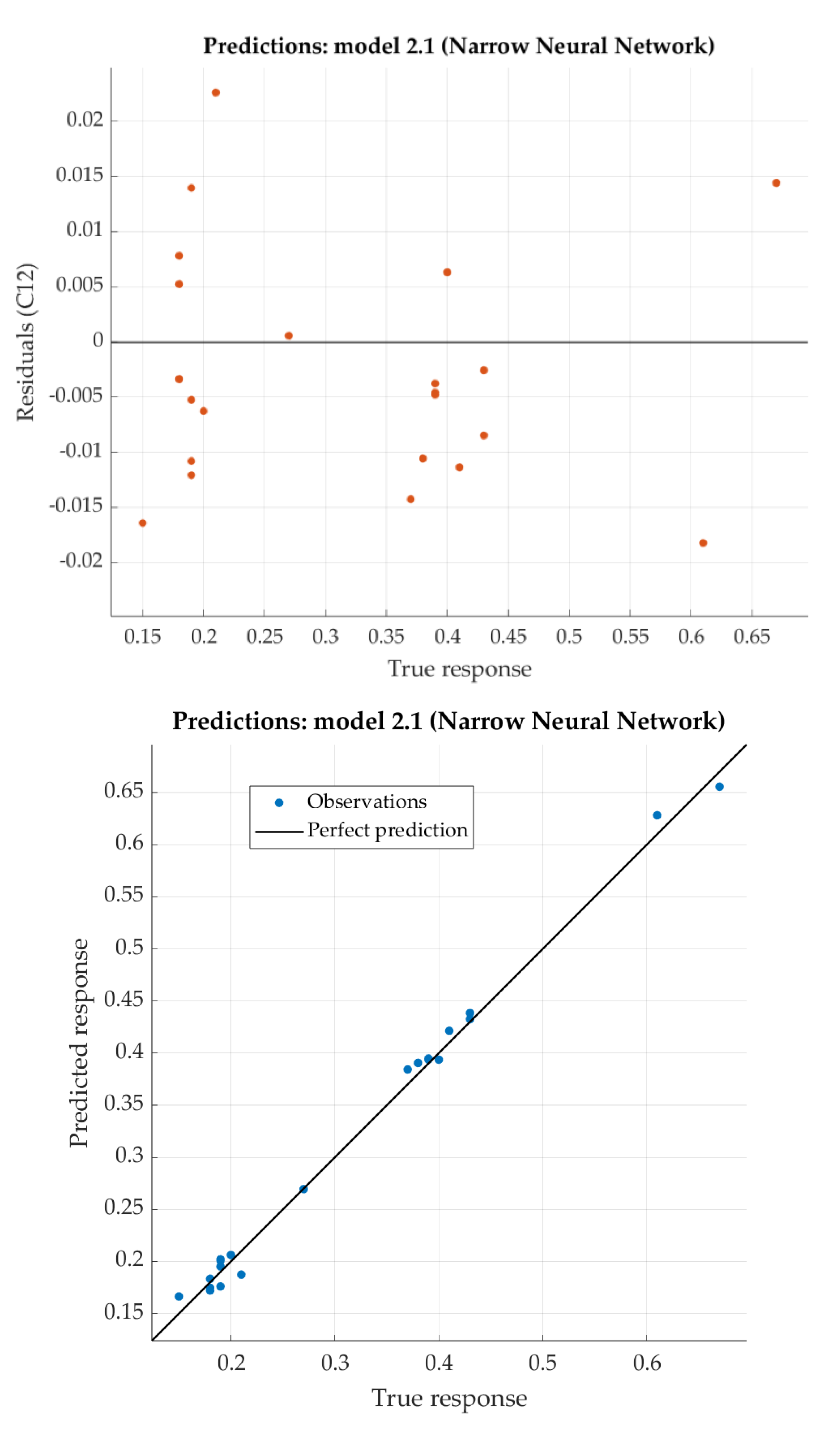
The Narrow Neural Network model has the best results (with one hidden layer with 10 nodes). For that model, the predicted response vs. the experimental data, for each observation (from the training dataset), is shown in Figure 5. For the same model, the predicted response vs. the experimental unseen data (the test dataset) are shown in Figure 6. In Figure 6 relation between residuals (difference between predicted response and experimental data) and true data are shown too. The best neural network model shows excellent results with very low RSME, as well as extremely high R² (close to 1).

3.1.2. Experimental Result Analysis for Manganese

The artificial neural network models for manganese are placed in Table 7 according to the lowest RMSE as well.

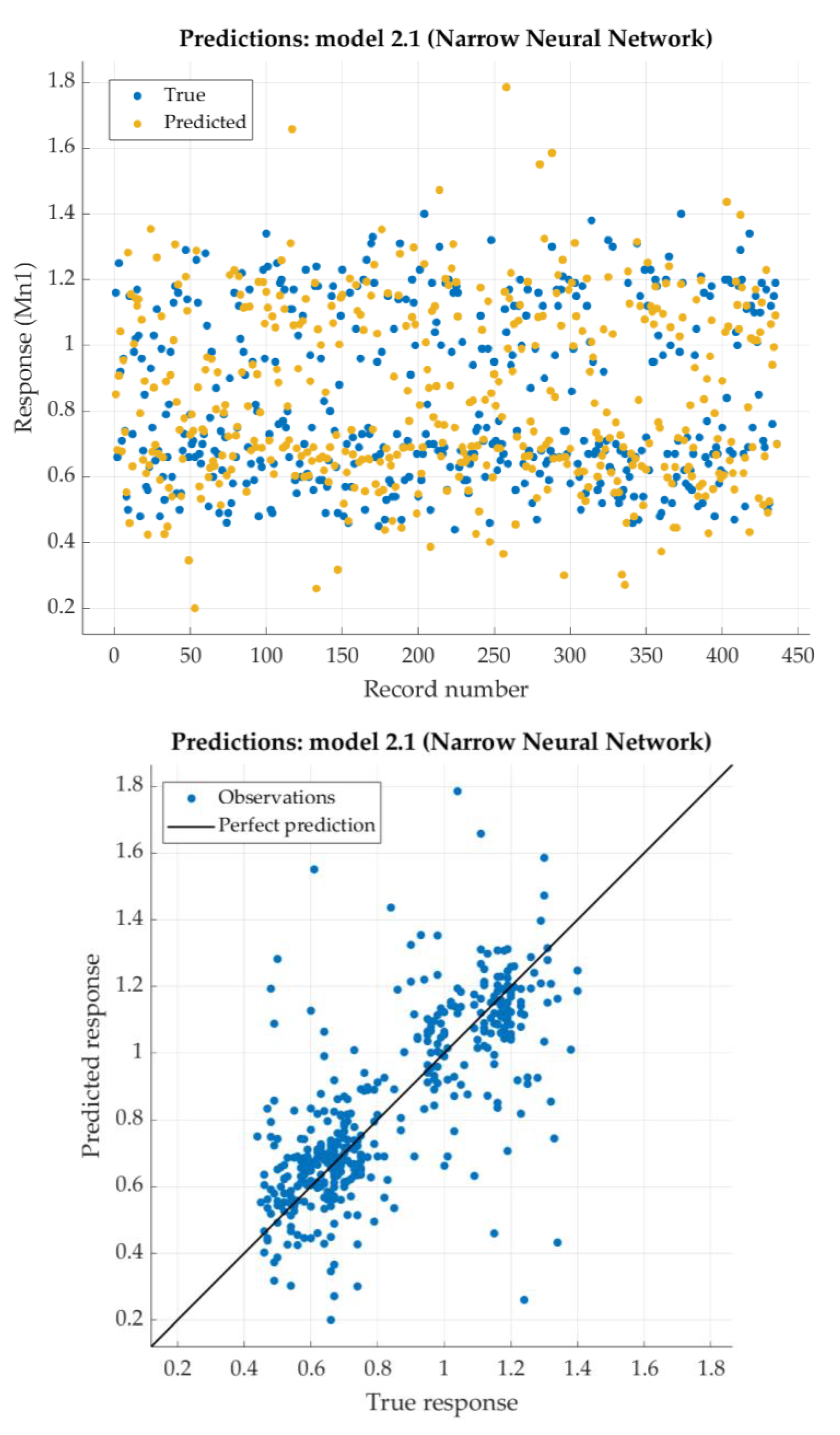
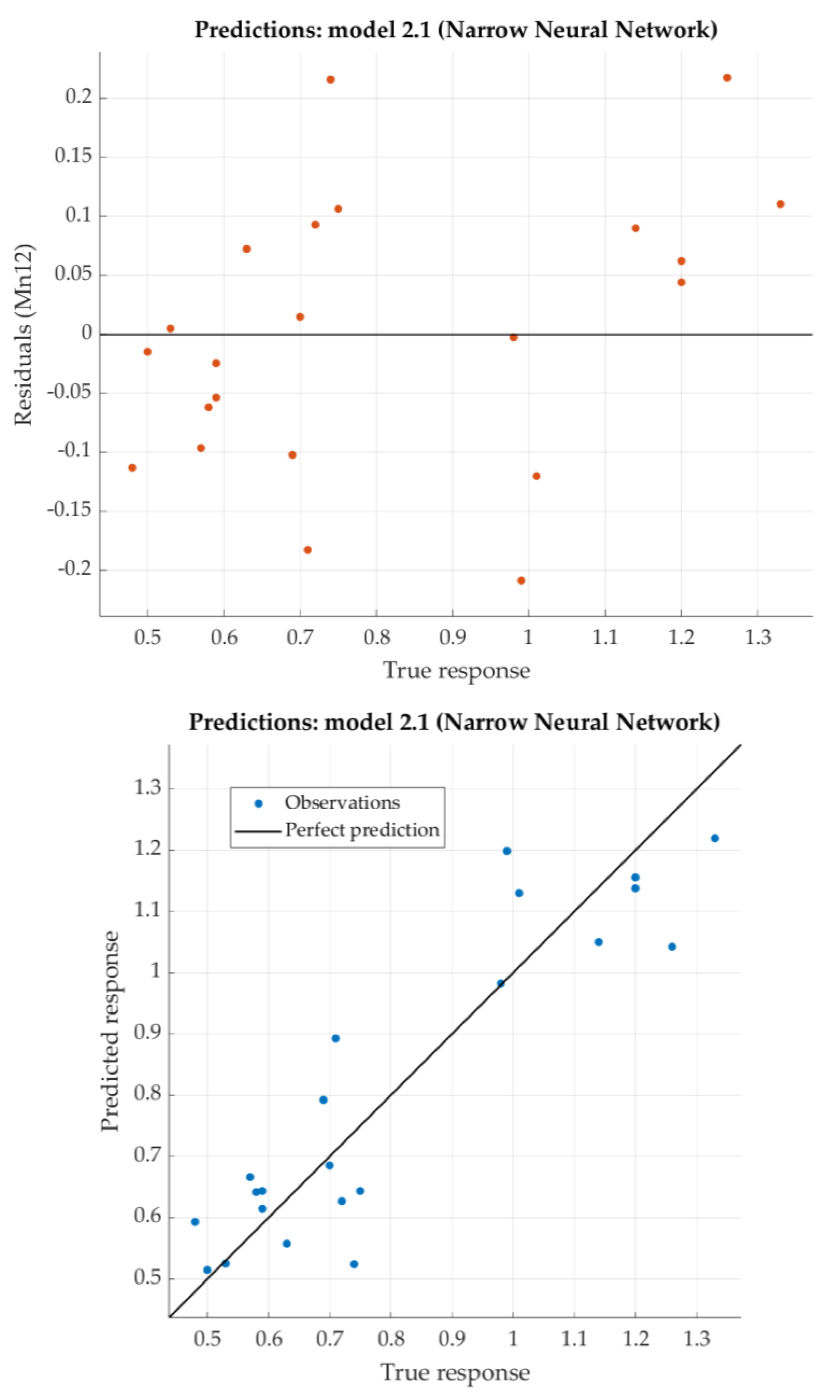
Like the results for carbon, the Narrow Neural Network model has the best results. The predicted response vs. the experimental data, for each observation (from the training dataset), is shown in Figure 7. For the same model, the predicted response vs. the experimental unseen data (the test dataset) are shown in Figure 8. In Figure 8, the relation between residuals and true data are shown too. The best neural network model shows good results with relatively low RSME, as well as with satisfying R².

3.1.3. Experimental Result Analysis for Silicon

The artificial neural network models for silicon are placed in Table 8 according to the lowest RMSE as well.

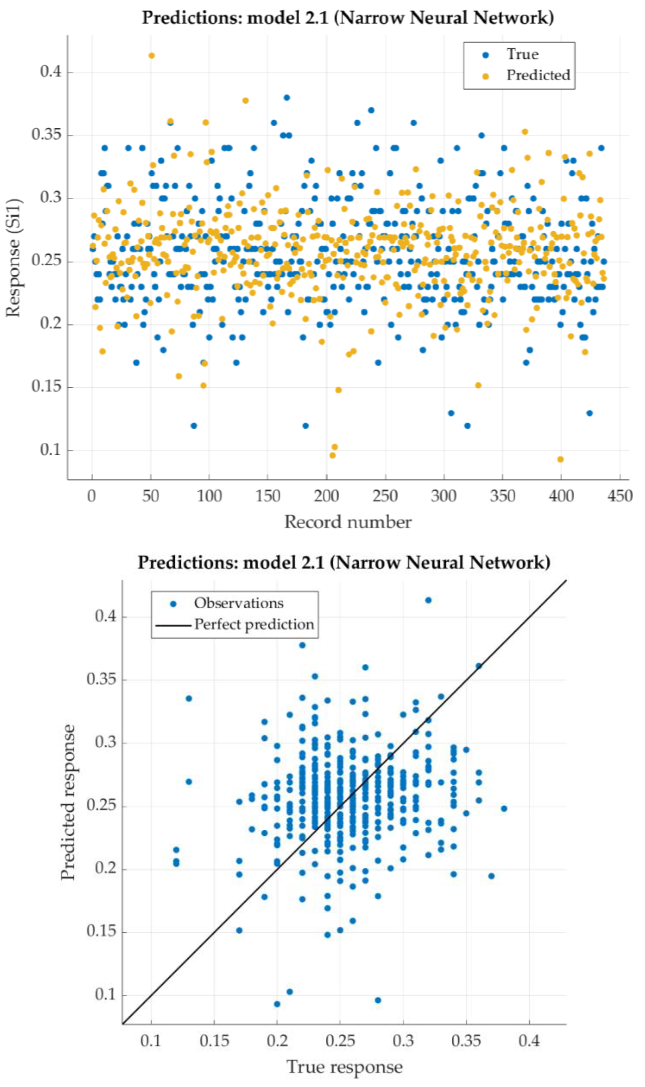
According to the given criterion (lowest RMSE), Optimizable Neural network is placed in first row (Table 8). However, predicted values of this model are concentrated around the mean value of trained dataset. Due to that, the best model is chosen the Narrow Neural Network model. For that model, the predicted response vs. 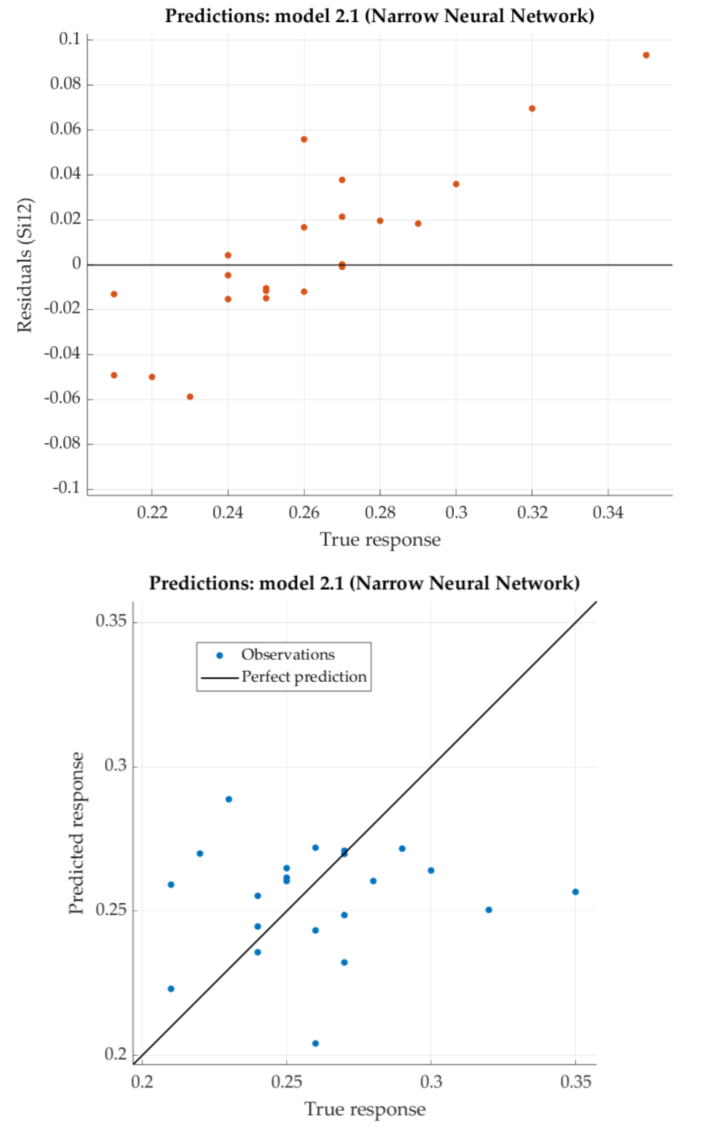the experimental data, for each observation from the training dataset, is shown in Figure 9. For the same model, the predicted response vs. the experimental unseen data is shown in Figure 10. In Figure 10, the relation between residuals and true data are shown too.

The Narrow Neural Network has very low RSME, so one can conclude that the model is very good. At the same time, the coefficient of determination R² is negative. By the definition, coefficient of determination can be negative, but it shows that the regression performed poorly, even worse when the regression model explains none of the variability of the response data around its mean [38]. Nevertheless, residuals in Figure 10 show very small figures. It means that predicted values are similar to the experimental data and that predicted data for silicon are within the given steel standard.

3.1.4. Experimental Result Analysis for Chromium

The artificial neural network models for chromium are placed in Table 9 according to the lowest RMSE as well.

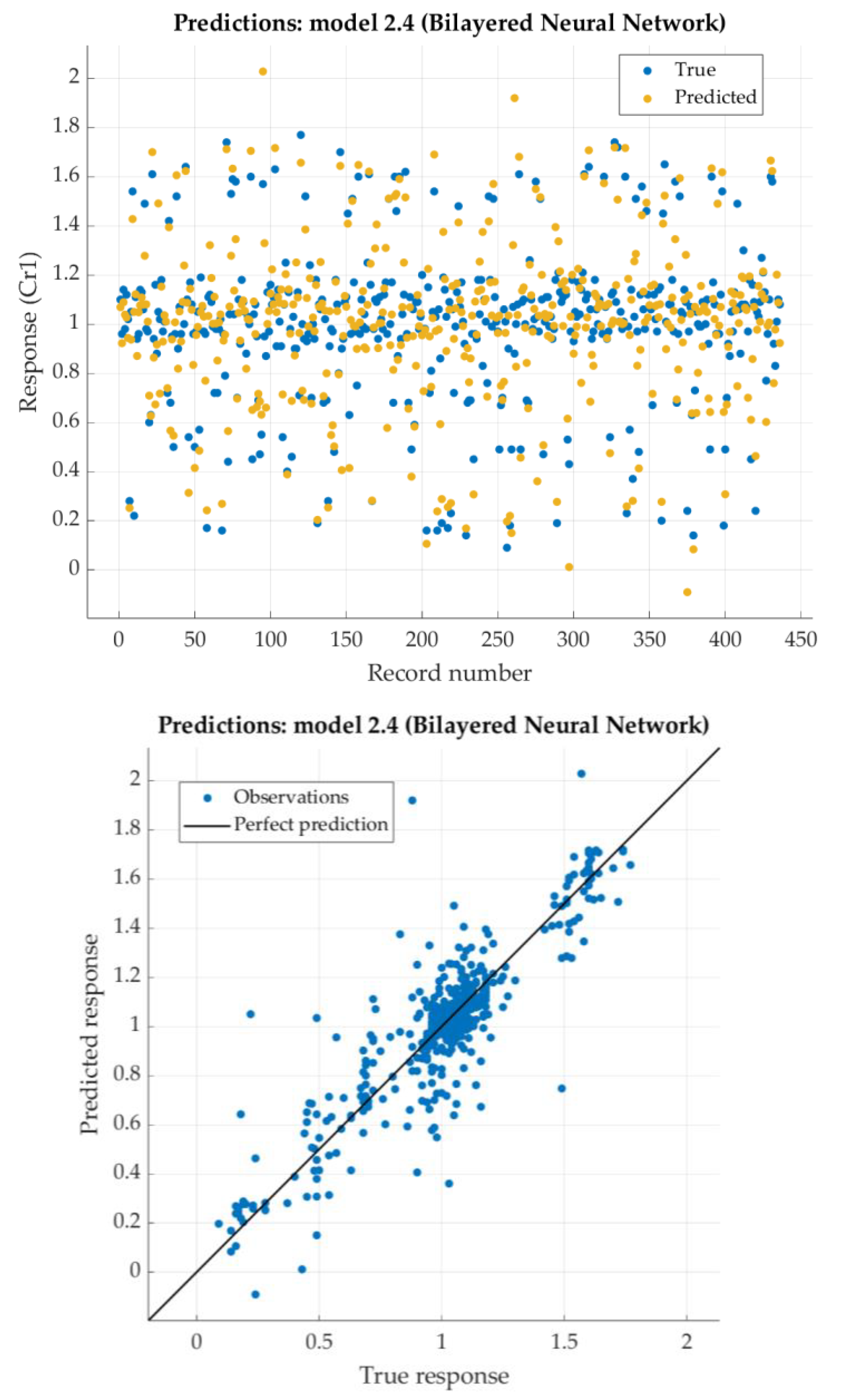
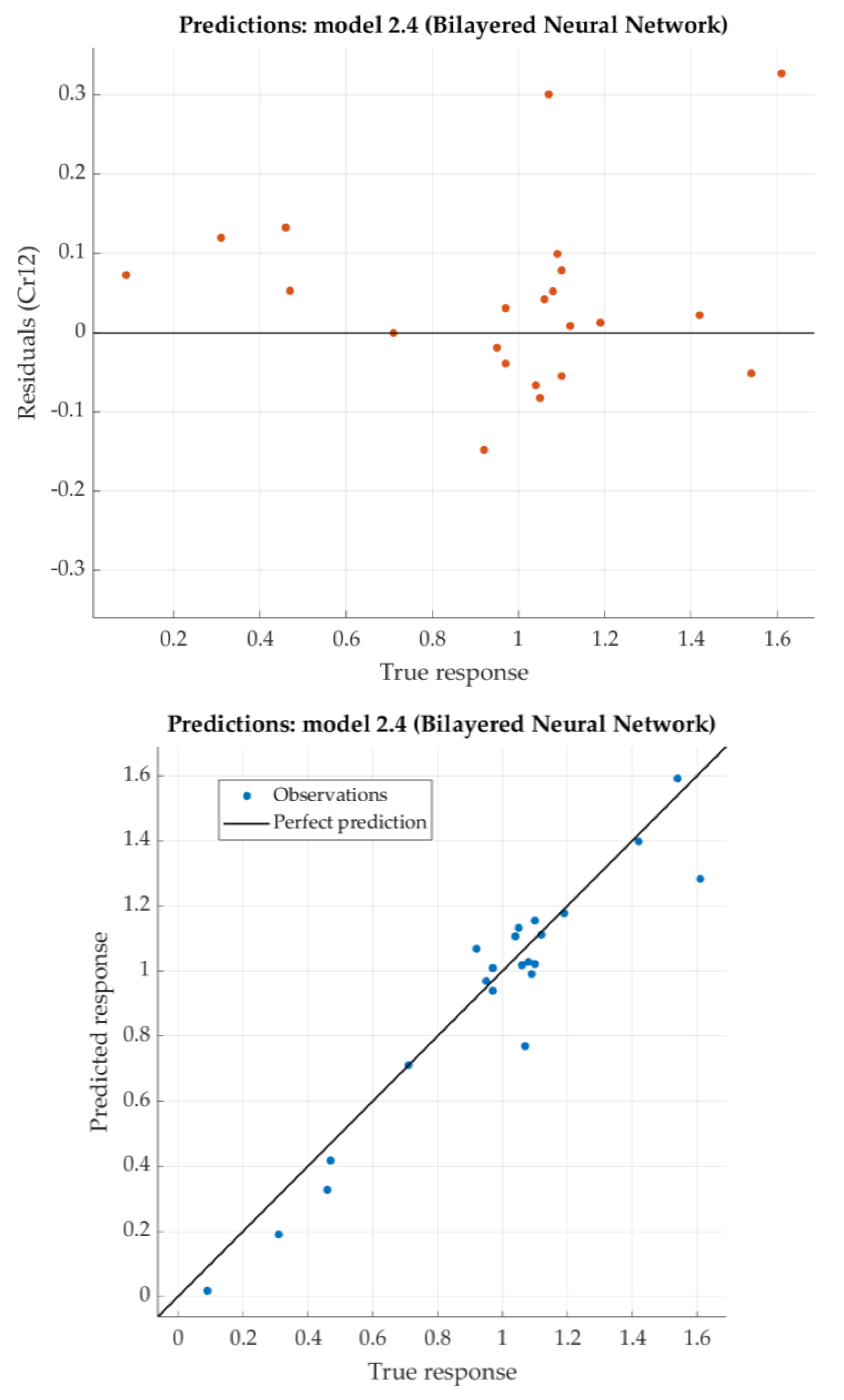
According to the given criterion, Bilayered Neural network model is chosen as the best (neural network with two hidden layers with 10 nodes each). For that model, the predicted response vs. the experimental data, for each observation from the training dataset, is shown in Figure 11. For the same model, the predicted response vs. the experimental unseen data is shown in Figure 12. In Figure 12, the relation between residuals and true data is shown too.

The Bilayered Narrow Neural Network has relatively low RSME and very good the coefficient of determination R² (close to 0.9).

3.1.5. Experimental Result Analysis for Nickel

The artificial neural network models for nickel placed in Table 10 according to the lowest RMSE.

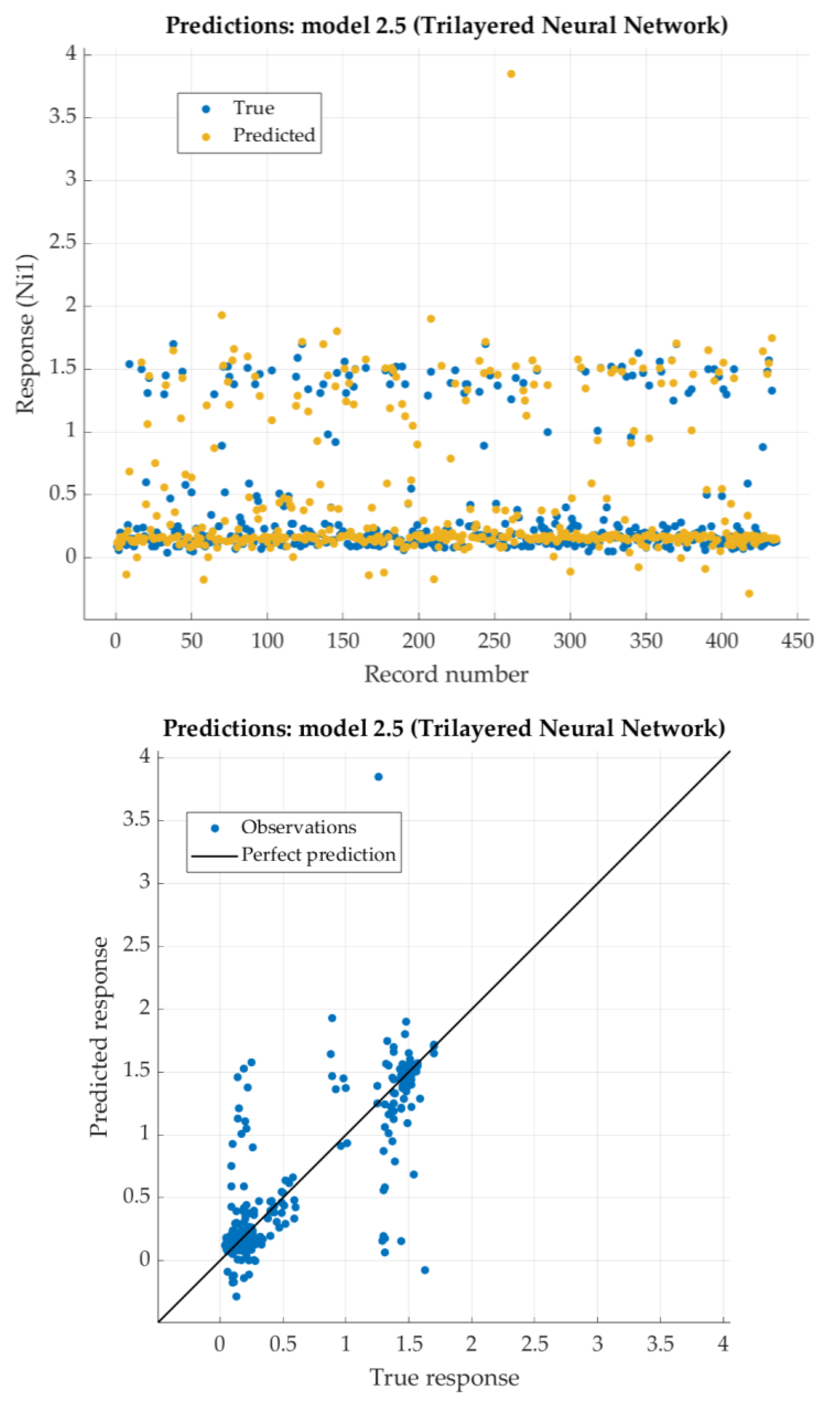
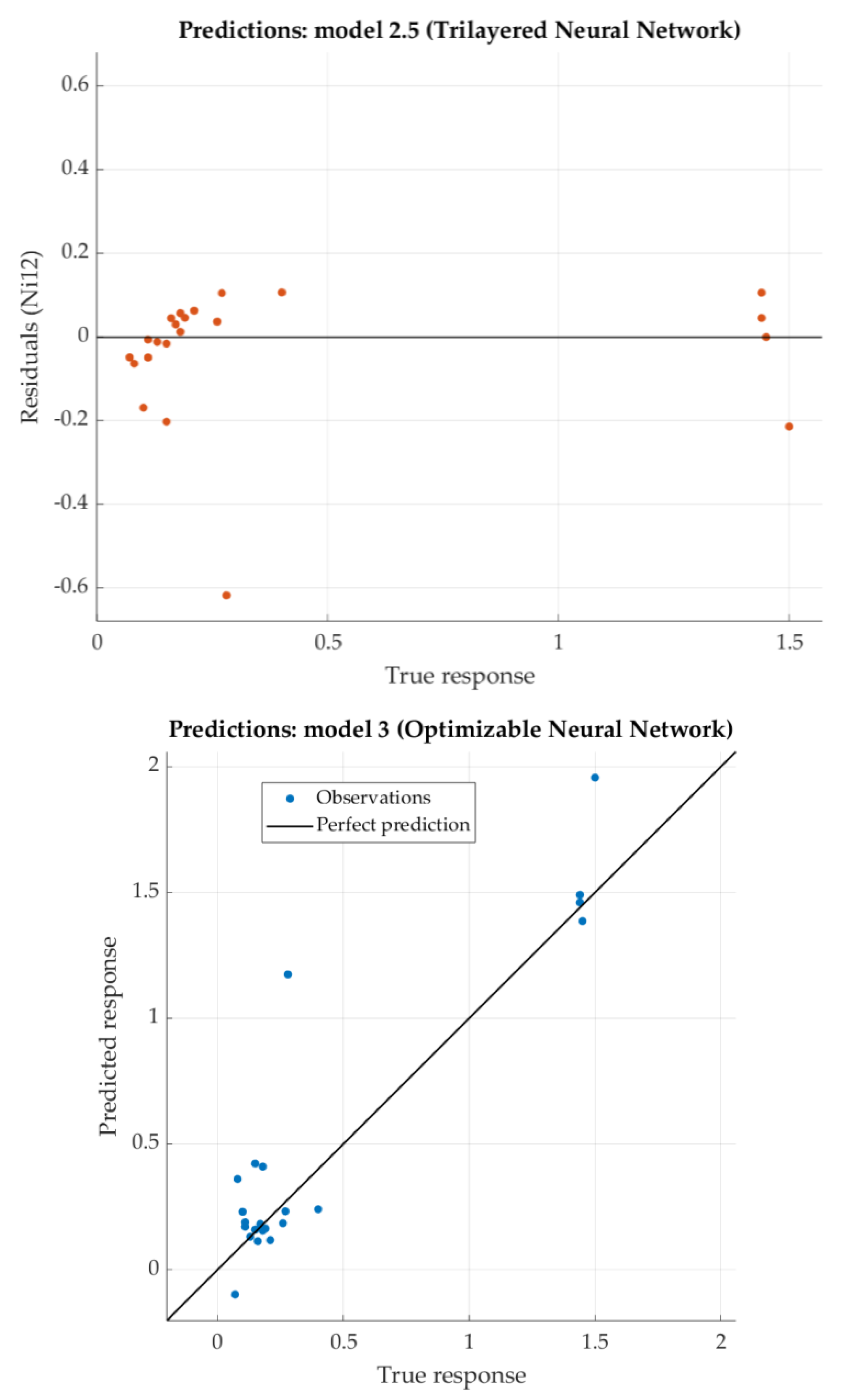
According to the given criterion, Trilayered Neural network model is chosen as the best (neural network with three hidden layers with 10 nodes each). For that model, the predicted response vs. the experimental data, for each observation from the training dataset, is shown in Figure 13. For the same model, the predicted response vs. the experimental unseen data is shown in Figure 14. In Figure 14, the relation between residuals and true data is shown too.

The Trilayered Narrow Neural Network has relatively low RSME and very good the coefficient of determination R² (close to 0.9). For most of the dataset, residuals are lower than 0.2 with one relatively high exception (0.6).

3.1.6. Experimental Result Analysis for Molybdenum

The artificial neural network models for molybdenum are placed in Table 11 according to the lowest RMSE as well.

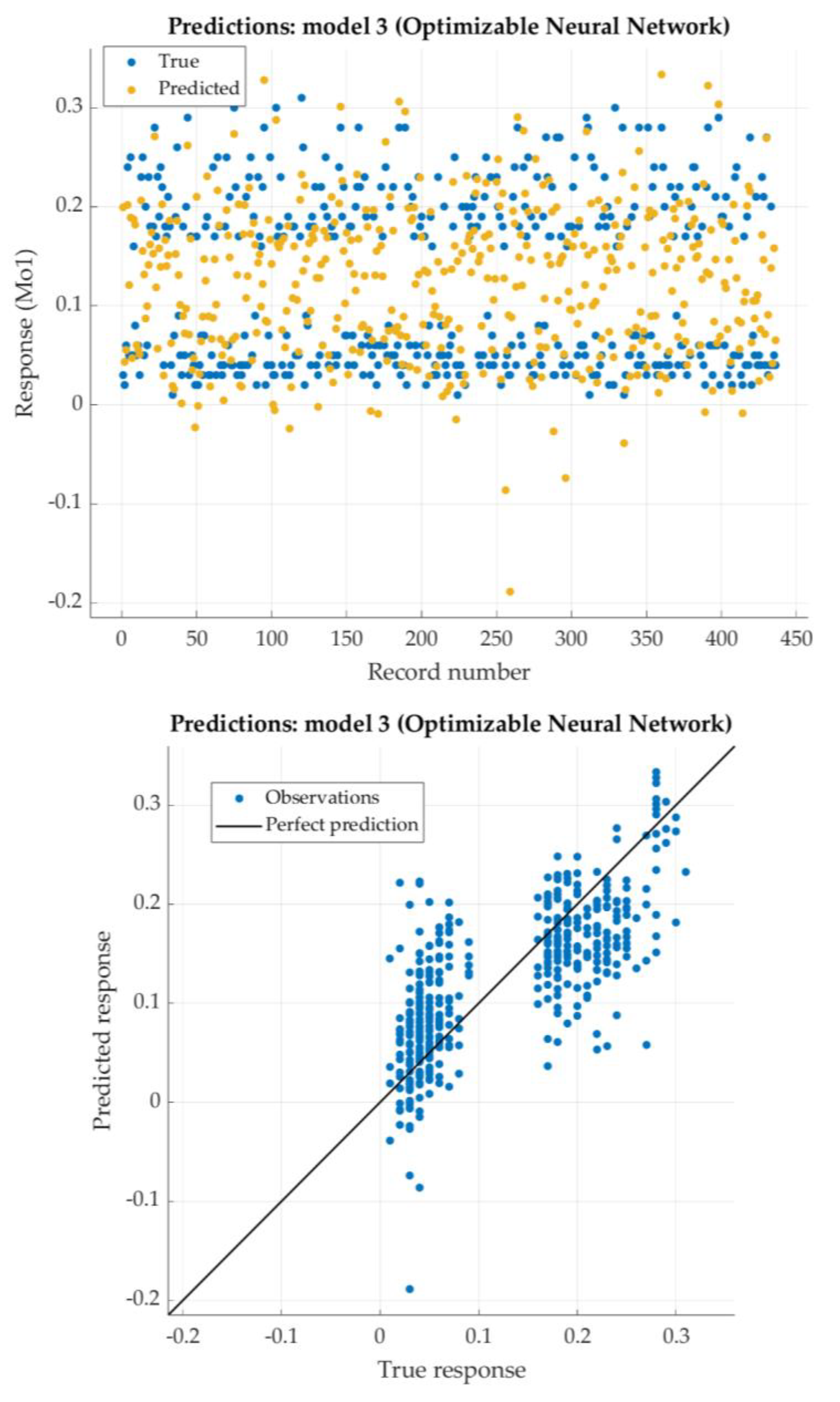
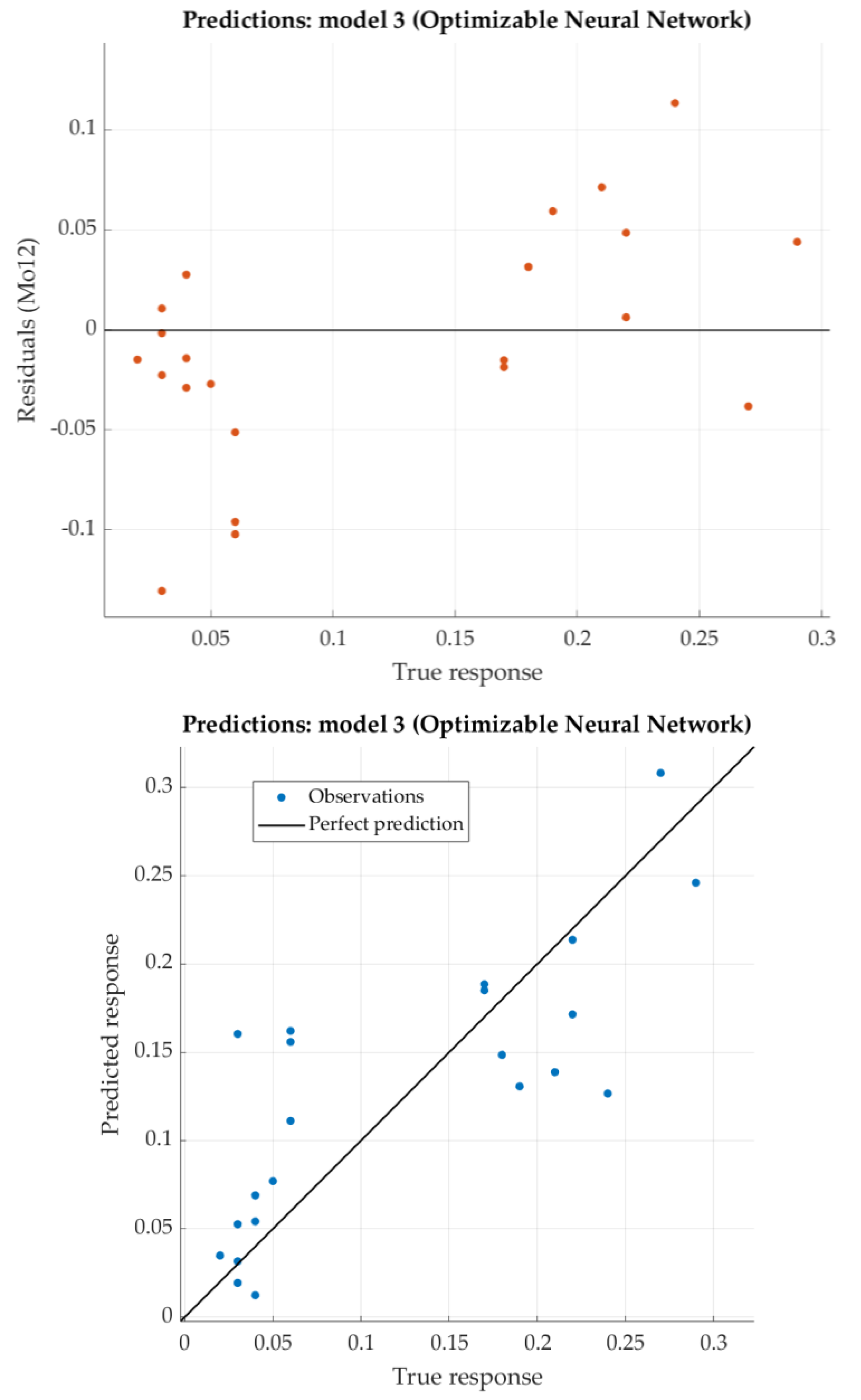
According to the given criterion, Optimizable Neural network model is chosen as the best (neural network with two hidden layers, first with 295 nodes and second with 5 nodes). For tha0t model, the predicted response vs. the experimental data, for each observation from the training dataset, is shown in Figure 15. For the same model, the predicted response vs. the experimental unseen data is shown in Figure 16. In Figure 16, the relation between residuals and true data is shown too.

The Optimizable Narrow Neural Network has very low RSME and weakly the coefficient of determination R². For most of the test dataset, residuals are lower than 0.1.

3.1.7. Experimental Result Analysis for Copper

The artificial neural network models for copper are placed in Table 12 according to the lowest RMSE as well.

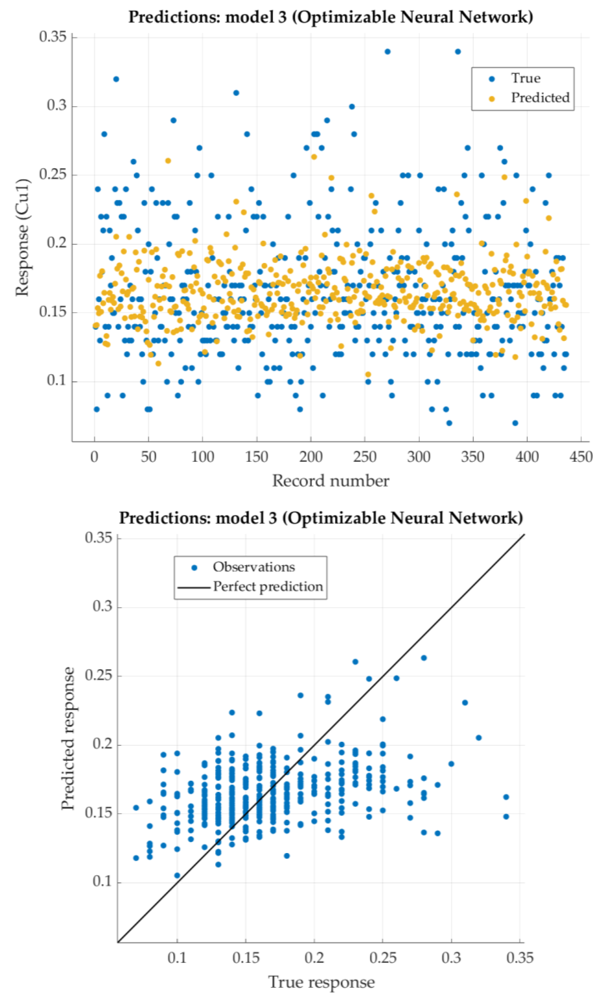
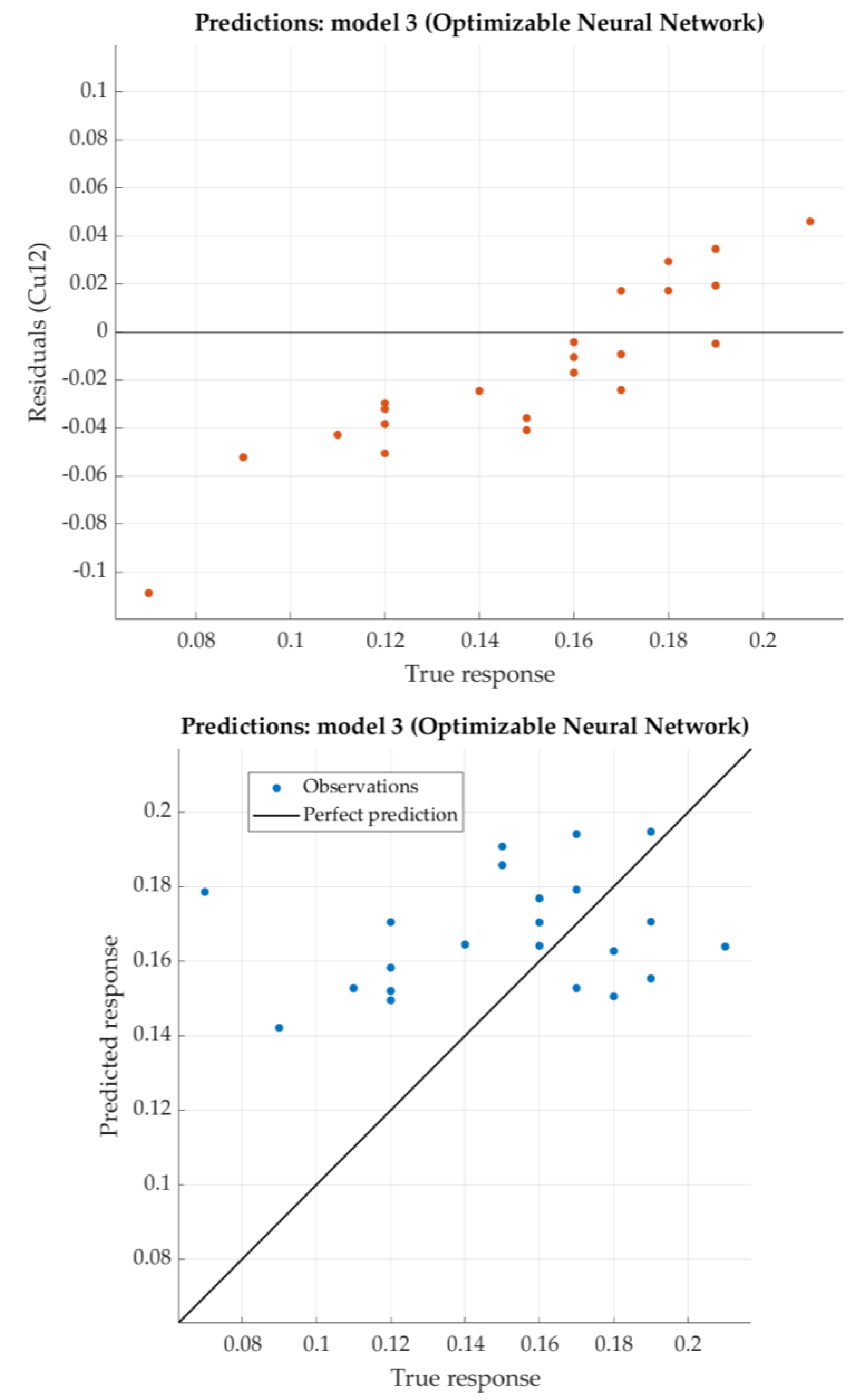
According to the given criterion (lowest RMSE), Optimizable Neural network is placed in first row (one hidden layer with 260 nodes). For that model, the predicted response vs. the experimental data, for each observation from the training dataset, is shown in Figure 17. For the same model, the predicted response vs. the experimental unseen data is shown in Figure 18. In Figure 18, the relation between residuals and true data are shown too.

The Optimizable Neural Network has very low RSME, while the coefficient of determination R² negative which shows that regression performed poorly. Nevertheless, residuals in Figure 18 show very small figures (lower than 0.1). It means that predicted values are similar to the experimental data.

3.1.8. Comparison of Predicted and Experimental Data

Predicted and experimental data for five different steels are given in Table 13. Steel C60E is chosen from EN 10083-2:2006 standard (Steels for quenching and tempering) as non-alloy steel. Alloy steels 41Cr4 and 46Cr2 are steel grades chosen from standard EN 10083-3:2006 (Steels for quenching and tempering). Steel 17CrNi6-6 is the steel grade chosen from standard EN 10084:2008 (Case hardening steels). Steel 65Mn4 is chosen as a steel grade which is not part of any standard. That steel shows relatively high values of hardness close to the quenched-end of Jominy specimen. The hardness declines after distance of only 7 mm from quenched-end of Jominy specimen, which can be characterized as low hardenability.

For each of those steels, according to the steel grades, minimum and maximum values for defined chemical elements are given too. Predicted values for chemical elements, for all steels, are within the limits defined by the steel grades.

4. Discussion

The given results for investigated alloying elements can be divided into three groups. The first group includes carbon, manganese and chromium. These elements are mandatory for almost all steel grades within the standards EN 10083-2, EN 10083-3, EN 10084 [33,34,35]. Results for these elements show excellent parameters: root mean square error (RMSE) and coefficient of determination (R²). Residual tests show very small differences between predicted and experimental values.

The second group includes nickel and molybdenum. Root mean square error for molybdenum is very little and residual test for that element show values lower than 0.1%. Root mean square error for nickel is also little, while coefficient of determination is 90%. Both of elements are mandatory for some steels grades within the researched standards. To improve the model more nickel and molybdenum steels (steels within which nickel and molybdenum are important alloying elements) should be included.

The third group includes silicon and copper. For all steel grades silicon is defined with maximum of 0.4%, while copper is not mandatory for any steel grade within the investigated standard [33,34,35]. RMSE for both elements show very good results. On the other side, the coefficient of determination is even below zero for silicon and close to 0 for copper. Silicon is not a carbide former and has small influence on hardenability. In low concentrations silicon is primarily used as a potent deoxidizer [29]. Only significant increase in mass content up to 0.75% enhances the hardenability [39]. Investigated steels have less than 0.35% of copper. Such a little amount of copper has little or no effect on hardenability.

5. Conclusions

The paper presents models of neural networks for designing chemical composition of steels for heat treatment. Neural networks models were developed based on 470 data that included the consecutive hardness values at 13 distances from the quenched-end of Jominy specimen and wt.% content of alloying elements C, Si, Mn, Cr, Ni, Mo and Cu. Complex regression analysis included presence of 50% of martensite in the microstructure.

Knowing the required hardenability of the machine part or tool is key prior to selection of material. To meet required hardenability, the optimal design of the chemical composition of the steel is necessary. Customers are often forced to choose a steel of a specific steel grade that can provide such hardenability. Often, that steel grade can have an excessive hardenability than required, which unnecessarily leads to a greater use of alloying elements. It is therefore important that the chemical composition should be designed according to the customer’s requirements, to obtain the required hardenability and relatively low production costs.

Developed artificial neural network models can be successfully used to predict the chemical composition of steels for heat treatment according to known curvature of Jominy curve. Predicted values for all seven chemical elements are close to experimental values and within the limits defined by the steel grades. To design any artificial neural network a relatively large number of experimental data is required. With additional experimental data, for nickel and molybdenum steels especially, used for learning and testing neural networks, proposed models can be further improved.

References

Liščić, B. Hardenability. In Steel Heat Treatment Handbook, 2nd ed; Totten, G.E.; CRC Press, Oregon, USA, 2007; pp. 213–276. [CrossRef]
Mesquita, R.A.; Schneider, R.E. Introduction to Heat Treating of Tool Steels. In ASM Handbook Volume 4D: Heat Treating of Irons and Steels, Dossett, J.L.; Totten, G.E.; ASM Int., Ohio, USA; 2014; pp. 277–287. [CrossRef]
Jominy, W.E.; Boegehold, A.L. A hardenability test for carburizing steel. Trans. ASM 1938, 26, 574–606. [Google Scholar]
ISO. 642: 1999 Steel– Hardenability Test by End Quenching (Jominy Test); International Organization for Standardization: Geneva, Switzerland, 1999. [Google Scholar]
ASTM. A255-10 Standard Test Methods for Determining Hardenability of Steel; ASTM International: West Conshohocken, USA, 2010. [Google Scholar]
JIS. G 0561 Method of Hardenability Test for Steel (End Quenching Method); Japanese Standards Association: Tokyo, Japan, 2006. [Google Scholar]
Grossmann, M.A.; Asimov, M.; Urba, S.F.; Hardenability, its relation to quenching and some quantitative data. Trans. ASM, 124-197.
Grossmann, M.A. Hardenability Calculated from Chemical Composition. AIME Transactions 155 1942, 227–255. [Google Scholar]
Crafts, W.; Lamont, J.L. Hardenability and Steel Selection. Pitman Publishing Corporation: Toronto, Canada, 1949; pp. 147–175.
Kramer, I.R.; Hafner, R.H. Effect of Sixteen Alloying Elements on Hardenability of Steel. 1944. [Google Scholar]
Comstock, G.F. ; The influence of titanium on the hardenability of steel. AIME Transactions. 1945, 1, 148–150. [Google Scholar]
Hodge, J.M.; Orehoski, M.A.; Relationship between the hardenability and percentage of carbon in some low alloy steels, AIME Transactions 167 1946, 627-642.
Brown, G.T.; James, B.A. The accurate measurement, calculation, and control of steel hardenability. Metall Trans 1973, 4, 2245–2256. [Google Scholar] [CrossRef]
Doane, D.V. Application of Hardenability Concepts in Heat Treatment of Steels. J. Heat Treating. 1979, 1, 5–30. [Google Scholar] [CrossRef]
Mangonon, P.L. ; Relative hardenabilities and interaction effects of Mo and V in 4330 alloy steel. Metall Trans A 1982, 13, 319–320. [Google Scholar] [CrossRef]
Tartaglia, J.M.; Eldis, G.T. Core Hardenability Calculations for Carburizing Steels. Metall Trans A 1984, 15, 1173–1183. [Google Scholar] [CrossRef]
Kasuya, T.; Yurioka, N. Carbon Equivalent and Multiplying Factor for Hardenability of Steel. In Proceedings of the The 72nd Annual AWS Meeting, Detroit, USA, 15-19 April 1991. [Google Scholar] [CrossRef]
Yamada, M.; Yan, L.; et al. Effects of Alloying Elements on the Hardenability, Toughness and the Resistance of Stress Corrosion Cracking in 1 to 3 mass % Cr Low Alloy Steel. ISIJ Int. 2014, 54, 240–247. [Google Scholar] [CrossRef]
Filetin, T.; Majetić, D. Žmak, I. In Prediction the Jominy curves by means of neural networks. In Proceedings of the 11th IFHTSE Congress, Florence, Italy, 19-21 Oct. 1998. [Google Scholar]
Dobrzanski, L.A.; Sitek, W. Application of a neural network in modelling of hardenability of constructional steels. J. Mater. Process. Technol. 1998, 78, 59–66. [Google Scholar] [CrossRef]
Bhadeshia, H.K.D.H. ; ‘Neural networks in materials science. ISIJ Int. 1999, 39, 966–979. [Google Scholar] [CrossRef]
Filetin, T.; Majetić, D.; Žmak, I. Application of Neural Networks in Predicting the Steel Properties. In Proceedings of the 10th International DAAAM Symposium, Vienna, Austria, 21-23 Oct. 1999. [Google Scholar]
Sitek, W.; Dobrzanski, L.A.; Zacłona, J. The modelling of high-speed steels’ properties using neural networks. J. Mater. Process. Technol 2004, 157–158, 245–249. [Google Scholar] [CrossRef]
Sitek, W. Methodology of High-Speed Steels Design Using the Artificial Intelligence Tools. J. Achiev. Mater. Manuf. Eng. 2010, 39, 115–160. [Google Scholar]
Sarker, I.H. Deep Learning: A Comprehensive Overview on Techniques, Taxonomy, Applications and Research Directions. SN Comput Sci. 2021 2, 420. [CrossRef]
Sitek, W.; Trzaska, J. Practical Aspects of the Design and Use of the Artificial Neural Networks in Materials Engineering. Metals. 2021, 11, 1832. [Google Scholar] [CrossRef]
Taherdoost, H. Deep Learning and Neural Networks: Decision-Making Implications. Symmetry 2023, 15, 1723. [Google Scholar] [CrossRef]
Hodge, J.M.; Orehoski, M.A.; Hardenability Effects in Relation to the Percentage of Martensite, AIME Transactions 167 1946, 502-512.
Canale, L.C.F.L.; Albano, L. Hardenability of Steel. In Comprehensive Materials Processing; Hashmi, S., Batalha, G.F.; Elsevier, 2014, Volume 12, pp. 39–97. [CrossRef]
Totten, G.E.; Bates, C.E. Handbook of Quenchants and Quenching Technology; ASM International: Materials Park, USA, 1993; pp. 35–68. [Google Scholar]
Smoljan, B.; Iljkić, D.; Tomašić, N. Mathematical modelling of Hardness of Quenched and Tempered Steel. Archives of Materials Science and Engineering 2015, 74, 85–93. [Google Scholar]
Liščić, B.; Steel Heat Treatment. In Steel Heat Treatment Handbook, 2nd ed; Totten, G.E.; CRC Press, Oregon, USA, 2007; pp. 277–414. [CrossRef]
European Committee for Standardization; EN 10083-2:2006 Steels for quenching and tempering—Part 2: Technical delivery conditions for non alloy Steels; German Institute for Standardization, Berlin, Germany, 2006.
European Committee for Standardization; EN 10083-3:2007 Steels for quenching and tempering—Part 3: Technical delivery conditions for alloy Steels; German Institute for Standardization, Berlin, Germany, 2007.
European Committee for Standardization; EN 10084:2008 Case hardening steels: Technical delivery conditions; German Institute for Standardization, Berlin, Germany, 2008.
Gemechu, W.F.; Sitek, W.; Batalha, G.F. Improving Hardenability Modeling: A Bayesian Optimization Approach to Tuning Hyperparameters for Neural Network Regression. Appl. Sci. 2024, 14, 2554. [Google Scholar] [CrossRef]
Massey, F.J. The Kolmogorov-Smirnov Test for Goodness of Fit. J. Am. Stat. Assoc. 1951, 46, 68–78. [Google Scholar] [CrossRef]
Chicco, D.; Warrens, M.J.; Jurman, G. 2021. The coefficient of determination R-squared is more informative than SMAPE, MAE, MAPE, MSE and RMSE in regression analysis evaluation. PeerJ Computer Sci. 2021. [CrossRef]
Wang, Z.; Qi, J.; Liu, Y. Effect of Silicon Content on the Hardenability and Mechanical Properties of Link-Chain Steel. J. of Materi Eng and Perform 2019, 28, 1678–1684. [Google Scholar] [CrossRef]

Figure 1. Required hardenability of the machine part vs. adequate hardenability of steel.

Figure 2. Ratio of hardness of steel with 50% martensite in the microstructure and 99% of martensite in the microstructure for different carbon content.

Figure 3. Predictors of steel 42CrMo4 (hardnesses and microstructures).

Figure 4. Training and test dataset’s split distribution

Figure 5. Performance evaluation of Narrow Neural Network on training dataset.

Figure 6. Performance evaluation of Narrow Neural Network on test dataset.

Figure 7. Performance evaluation of Narrow Neural Network on training dataset.

Figure 8. Performance evaluation of Narrow Neural Network on test dataset.

Figure 9. Performance evaluation of Narrow Neural Network on training dataset.

Figure 10. Performance evaluation of Narrow Neural Network on test dataset.

Figure 11. Performance evaluation of Bilayered Neural Network on training dataset.

Figure 12. Performance evaluation of Bilayered Narrow Neural Network on test dataset.

Figure 13. Performance evaluation of Trilayered Neural Network on training dataset.

Figure 14. Performance evaluation of Trilayered Narrow Neural Network on test dataset.

Figure 15. Performance evaluation of Optimized Neural Network on training dataset.

Figure 16. Performance evaluation of Optimized Narrow Neural Network on test dataset.

Figure 17. Performance evaluation of Narrow Neural Network on training dataset.

Figure 18. Performance evaluation of Optimized Narrow Neural Network on test dataset.

Table 1. Ranges of predictor parameters (HRC) used to model chemical composition of steels.

	HRC_1,5	HRC₃	HRC₅	HRC₇	HRC₉	HRC₁₁	HRC₁₃	HRC₁₅	HRC₂₀	HRC₂₅	HRC₃₀	HRC₄₀	HRC₅₀
Min.	64.5	64	63	61	60	59,5	59	58	57	56	54	51	44
Max.	38.5	36,75	26	21,5	20,5	19	18	17	15	13	12	11	10

Table 2. Predictors for one observation (steel 42CrMo4).

M_1,5	M₃	M₅	M₇	M₉	M₁₁	M₁₃	M₁₅	M₂₀	M₂₅	M₃₀	M₄₀	M₅₀
1	1	1	1	1	1	1	1	0	0	0	0	0

Table 3. Responses for steel 42CrMo4 (chemical composition).

C	Mn	Si	Cr	Ni	Mo	Cu
0.4	0.7	0.2	1.01	0.16	0.16	0.2

Table 4. Kolmogorov-Smirnov test results od goodness of fit of the training and test dataset.

Features	HRC_1,5	HRC₃	HRC₅	HRC₇	HRC₉	HRC₁₁	HRC₁₃	HRC₁₅	HRC₂₀	HRC₂₅	HRC₃₀	HRC₄₀	HRC₅₀
KS -test value	0.152	0.163	0.166	0.127	0.093	0.090	0.147	0.161	0.157	0.132	0.132	0.167	0.147
p-value	0.68	0.6	0.57	0.86	0.99	0.99	0.72	0.61	0.64	0.82	0.84	0.57	0.73

Table 5. Kolmogorov-Smirnov test results od goodness of fit of the training and test dataset.

Features	M_1,5	M₃	M₅	M₇	M₉	M₁₁	M₁₃	M₁₅	M₂₀	M₂₅	M₃₀	M₄₀	M₅₀
KS -test value	0	0	0.018	0.106	0.071	0	0.001	0.037	0.031	0.027	0.044	0.037	0.009
p-value	1	1	1	0.96	1	1	1	1	1	1	1	1	1

Table 6. Results after training for carbon with six different architectures of ANNs.

Model	Architecture	RMSE		R²		MAE	MSE
Model	Architecture	Train	Test	Train	Test	Test	Test
Narrow NN	26-10-1	0.0204	0.0108	0.973	0.994	0.0093	0.0001
Bilayered NN	26-10-10-1	0.0191	0.0114	0.976	0.994	0.0085	0.0001
Trilayered NN	26-10-10-10-1	0.0218	0.0140	0.969	0.991	0.0111	0.0002
Medium NN	26-25-1	0.0200	0.0199	0.974	0.981	0.0137	0.0004
Wide NN	26-100-1	0.0292	0.0290	0.945	0.959	0.0164	0.0008
Optimizable NN	26-4-4-14-1	0.0232	0.0307	0.965	0.954	0.0202	0.0010

Table 7. Results after training for manganese with six different architectures of ANNs.

Model	Architecture	RMSE		R²		MAE	MSE
Model	Architecture	Train	Test	Train	Test	Test	Test
Narrow NN	26-10-1	0.1870	0.1122	0.485	0.823	0.0915	0.0126
Trilayered NN	26-10-10-10-1	0.1930	0.1163	0.451	0.810	0.0827	0.0135
Wide NN	26-100-1	0.2084	0.1251	0.361	0.780	0.0885	0.0157
Optimizable NN	26-3-1	0.1637	0.1362	0.605	0.739	0.1188	0.0186
Medium NN	26-25-1	0.2110	0.1665	0.344	0.610	0.1222	0.0277
Bilayered NN	26-10-10-1	0.2389	0.1918	0.160	0.482	0.1092	0.0368

Table 8. Results after training for silicon with six different architectures of ANNs.

Model	Architecture	RMSE		R²		MAE	MSE
Model	Architecture	Train	Test	Train	Test	Test	Test
Optimizable NN	26-5-1	0.0426	0.0342	-0.011	-0.072	0.0258	0.0012
Narrow NN	26-10-1	0.0515	0.0371	-0.476	-0.262	0.0279	0.0014
Bilayered NN	26-10-10-1	0.0645	0.0401	-1.317	-0.474	0.0317	0.0016
Trilayered NN	26-10-10-10-1	0.0717	0.0428	-1.864	-0.678	0.0333	0.0018
Wide NN	26-100-1	0.0757	0.0510	-2.192	-1.387	0.0392	0.0026
Medium NN	26-25-1	0.0622	0.0630	-1.152	-2.642	0.0405	0.0040

Table 9. Results after training for chromium with six different architectures of ANNs.

Model	Architecture	RMSE		R²		MAE	MSE
Model	Architecture	Train	Test	Train	Test	Test	Test
Bilayered NN	26-10-10-1	0.1609	0.1168	0.748	0.896	0.1047	0.0824
Optimizable NN	26-219-1	0.1308	0.1377	0.834	0.856	0.0939	0.0886
Trilayered NN	26-10-10-10-1	0.1518	0.1400	0.776	0.851	0.0963	0.1009
Wide NN	26-100-1	0.1539	0.1447	0.770	0.841	0.1033	0.0839
Narrow NN	26-10-1	0.1433	0.1748	0.800	0.767	0.1006	0.1310
Medium NN	26-25-1	0.1814	0.2039	0.680	0.684	0.1196	0.1304

Table 10. Results after training for nickel with six different architectures of ANNs.

Model	Architecture	RMSE		R²		MAE	MSE
Model	Architecture	Train	Test	Train	Test	Test	Test
Trilayered NN	26-10-10-10-1	0.2998	0.1590	0.660	0.899	0.0933	0.0253
Bilayered NN	26-10-10-1	0.3476	0.2386	0.544	0.771	0.1416	0.0569
Optimizable NN	26—1	0.2800	0.2450	0.704	0.759	0.1451	0.0600
Wide NN	26-100-1	0.3841	0.2715	0.443	0.704	0.1524	0.0737
Narrow NN	26-10-1	0.3537	0.3381	0.527	0.541	0.1986	0.1143
Medium NN	26-25-1	0.4303	0.3608	0.301	0.477	0.2241	0.1302

Table 11. Results after training for molybdenum with six different architectures of ANNs.

Model	Architecture	RMSE		R²		MAE	MSE
Model	Architecture	Train	Test	Train	Test	Test	Test
Optimizable NN	26-295-5-1	0.0611	0.0570	0.5160	0.613	0.0442	0.0033
Trilayered NN	26-10-10-10-1	0.0871	0.0634	0.0147	0.521	0.0417	0.0040
Bilayered NN	26-10-10-1	0.2185	0.0682	-5.1983	0.445	0.0461	0.0047
Narrow NN	26-10-1	0.0798	0.0701	0.1732	0.415	0.0591	0.0049
Wide NN	26-100-1	0.1012	0.0832	-0.3292	0.176	0.0558	0.0069
Medium NN	26-25-1	0.1009	0.1070	-0.3205	-0.364	0.0787	0.0115

Table 12. Results after training for copper with six different architectures of ANNs.

Model	Architecture	RMSE		R²		MAE	MSE
Model	Architecture	Train	Test	Train	Test	Test	Test
Optimizable NN	26-260-1	0.0442	0.0020	0.1505	0.0331	0.0297	0.0013
Narrow NN	26-10-1	0.0613	0.0038	-0.6341	0.0452	0.0433	0.0036
Medium NN	26-25-1	0.0659	0.0043	-0.8875	0.0462	0.0443	0.0042
Trilayered NN	26-10-10-10-1	0.0536	0.0029	-0.2493	0.0394	0.0516	0.0049
Wide NN	26-100-1	0.0741	0.0055	-1.3885	0.0500	0.0562	0.0052
Bilayered NN	26-10-10-1	0.0738	0.0055	-1.3784	0.0457	0.0639	0.0098

Table 13. Predicted vs. experimental data for content of chemical elements.

	Steel	C60E	41Cr4	46Cr2	17CrNi6-6	65Mn4
C	Pred. vs. exp. values	0.63 0.61	0.43 0.43	0.44 0.43	0.17 0.15	0.66 0.67
C	Steel grade limits	0.57 – 0.65	0.38 0.45	0.42 – 0.50	0.14 – 0.2	0.6 – 0.7
Mn	Pred. vs. exp. values	0.79 0.69	0.63 0.72	0.64 0.75	0.53 0.53	1.13 1.01
Mn	Steel grade limits	0.6 – 0.9	0.6 – 0.9	0.50 – 0.80	0.5 – 0.9	0.9 – 1.2
Si	Pred. vs. exp. values	0.26 0.24	0.27 0.27	0.20 0.26	0.27 0.22	0.25 0.32
Si	Steel grade limits	0 – 0.4	0 – 0.4	0 – 0.40	0 – 0.4	0.25 – 0.50
Cr	Pred. vs. exp. values	0.19 0.31	0.99 1.09	0.42 0.47	1.4 1.42	0.02 0.09
Cr	Steel grade limits	0 – 0.4	0.9 – 1.2	0.4 – 0.6	1.4 – 1.7	N/D
Ni	Pred. vs. exp. values	0.12 0.11	0.17 0.15	0.29 0.40	1.45 – 1.45	0.12 0.07
Ni	Steel grade limits	0 – 0.4	N/D*	N/D*	1.4 – 1.7	N/D*
Mo	Pred. vs. exp. values	0.02 0.03	0.16 0.06	0.01 0.04	0.55 0.04	0.03 0.02
Mo	Steel grade limits	0 – 0.1	N/D*	N/D*	N/D*	N/D*
Cu	Pred. vs. exp. values	0.19 0.19	0.18 0.16	0.19 0.17	0.15 0.17	0.19 0.15
Cu	Steel grade limits	N/D*	N/D*	N/D*	N/D*	N/D*

* N/D not defined limits within the steel grade.

Disclaimer/Publisher’s Note: The statements, opinions and data contained in all publications are solely those of the individual author(s) and contributor(s) and not of MDPI and/or the editor(s). MDPI and/or the editor(s) disclaim responsibility for any injury to people or property resulting from any ideas, methods, instructions or products referred to in the content.

© 2024 by the authors. Licensee MDPI, Basel, Switzerland. This article is an open access article distributed under the terms and conditions of the Creative Commons Attribution (CC BY) license (http://creativecommons.org/licenses/by/4.0/).

Copyright: This open access article is published under a Creative Commons CC BY 4.0 license, which permit the free download, distribution, and reuse, provided that the author and preprint are cited in any reuse.

MDPI Initiatives

Important Links

Choose an area of interest and we will send you notifications of new preprints at your preferred frequency.

Disclaimer