Comparison of Using GeoGebra and Python to Discover the Motion of Device in a Well-Known Physical Experimental Instrument—Looking into Vibration-Damping Devices in the Scanning Tunneling Microscope

Preprint

Article

Comparison of Using GeoGebra and Python to Discover the Motion of Device in a Well-Known Physical Experimental Instrument—Looking into Vibration-Damping Devices in the Scanning Tunneling Microscope

Altmetrics

Downloads

Views

Comments

This version is not peer-reviewed

Submitted:

01 August 2024

Posted:

02 August 2024

You are already at the latest version

Alerts

Abstract

In this study, we focus on the vibration-damping devices within the renowned physical experimental apparatus—STM. Utilizing GeoGebra software and Python, we meticulously elucidate the principle by which the vibrations of the damper are damped in a magnetic field, thereby achieving the vibration-damping functionality of the entire system. This approach not only fosters a clear physical conceptualization but also ensures the acquisition of accurate and comprehensive knowledge. Furthermore, the inquiry demonstrates the process of problem clarification facilitated by the use of software tools and then we compare the power of the widlely programming language--Python and the GeoGebra.

Keywords:

Subject: Social Sciences - Education

The integration of modern educational techniques and programming languages is increasingly enhancing the teaching and exploration of physics problems. GeoGebra, a versatile mathematical software, stands out as a prevalent educational technology tool that aids in the investigation of physics issues. It has the capability to visualize the dynamic evolution of physical models, which significantly enriches students’ comprehension of the underlying physical principles [1]. Additionally, Python, a programming language celebrated for its widespread adoption, plays a pivotal role in this context and it’s an even more powerful tools to assist with learning...

This suite of tools is instrumental in tackling the abstract and intricate challenges within the field of physics. They facilitate an intuitive visual approach to learning, thereby bolstering students’ intuitive grasp of concepts. As following, the modeled problem is presented initially to streamline the illustration process and to aid the readers’ comprehension.

1. Presentation of the question after modeling

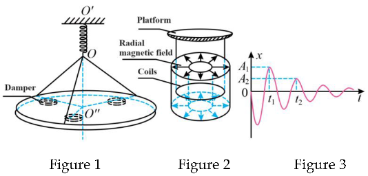
As shown in Figure 1, the scanning tunneling microscope vibration-damping device consists of an insulated vibration-damping platform and a magnetic damping damper. The platform is suspended by three identical light rods symmetrically distributed about the O’O’‘ axis at the lower end O of a lightweight spring, the upper end of the spring is fixedly suspended at the point O’, and three identical dampers symmetrically placed about the O’O ‘‘ axis symmetrically placed dampers are located below the platform. As shown in Figure 2, each damper consists of a coil fixed on the lower surface of the platform by an insulated light rod and a ferromagnet fixed on the tabletop that can generate a radial magnetic field, and the distribution of the radial magnetic field is symmetric about the center of the coil, and the magnitude of the magnetic induction at the coil is B. When the platform at rest is perturbed by the outside world, the coil makes a damping motion in the vertical direction in the magnetic field, and the image of its displacement change with time is shown in Figure 3. As shown in Figure 3. It is known that the velocity at t=0 is v₀, the direction is downward, t₁, t₂ time amplitudes are A₁, A₂. The total mass of the platform and the three coils is m, the coefficient of the strength of the spring is k, the radius of each coil is r, and the resistance is R. When the spring deformation variable is Δx, its elastic potential energy is.

\frac{1}{2} k Ä x^{2}

The elastic potential energy of the spring is Δx. Excluding air resistance, find the law of its motion.

2. Analytical Modeling and the Visualization of GeoGebra and Python

2.1. Theoretical Modeling Process

Statement: In the analysis, we conducted a comprehensive force analysis on the damper within the damping system to ascertain the forces acting upon it. These forces include the spring’s elastic force, the amperometric resistance which varies inversely with velocity, and the gravitational force exerted by the system. We established the x-axis with the spring’s original length at the coordinate origin, using OO’ as the positive direction. At any given instant, the velocity of the coil is denoted by v, and the spring’s stiffness coefficient is represented by k=k₁. From this setup, we can derive the following equations:

The component force of the spring in the vertical direction

T = k_{1} (Δ x_{0} - x)

Gravity of the system

G = - m g

For the amperometric resistance to the damper as a whole, At any instant, the current in a coil is

I = \frac{B (2 π r) v}{R} = \frac{2 π r B}{R} \frac{d x}{d t}

Then, the amperometric resistance to a coil is

F = - I \times 2 π r B = - \frac{B^{2} {(2 π r)}^{2} v}{R} = - \frac{4 π^{2} r^{2} B^{2}}{R} \frac{d x}{d t}

Therefore, the combined force in the system is

F_{t o t} = G + T + 3 F = - \frac{12 π^{2} r^{2} B^{2}}{R} \frac{d x}{d t} + k_{1} (Δ x_{0} - x) - m g

it follows that

m \frac{d^{2} x}{d t^{2}} = - \frac{12 π^{2} r^{2} B^{2}}{R} \frac{d x}{d t} + k_{1} (Δ x_{0} - x) - m g

Noting that Δx₀ is the elongation of the spring when the platform is balancing, then

k_{1} Δ x_{0} = m g

, therefore:

m \frac{d^{2} x}{d t^{2}} + \frac{12 π^{2} r^{2} B^{2}}{R} \frac{d x}{d t} + k_{1} x = 0

We let

{ω_{0}}^{2} = \frac{k_{1}}{m}, 2 δ = \frac{12 π^{2} r^{2} B^{2}}{m R}

, then the above equation reduce to

\frac{d^{2} x}{d t^{2}} + 2 δ \frac{d x}{d t} + {ω_{0}}^{2} x = 0

This equation represents a second-order linear differential equation characterized by constant coefficients. The nature of its solution is contingent upon the comparative magnitudes of the two variables, δ and ω₀ , present within the equation. Through rigorous mathematical computation, it is demonstrated that the oscillatory motion of the system’s displacement over time can be articulated.[2]:

x = A_{0} e^{- δ t} \cos (ω_{f} t + φ_{f})

which

ω_{f} = \sqrt{{ω_{0}}^{2} - δ^{2}} = \sqrt{\frac{k_{1}}{m} - \frac{36 π^{4} r^{4} B^{4}}{m^{2} R^{2}}}

A₀ and φ_f in the above equation are determined by the initial conditions of the whole system oscillator:

\{\begin{cases} x_{0} = A_{0} \cos φ_{f} \\ v_{0} = - δ A_{0} \cos φ_{f} - ω_{f} A_{0} \sin φ_{f} = - δ x_{0} - ω_{f} A_{0} \sin φ_{f} \end{cases}

So we can get that:

\{\begin{cases} A_{0} = \sqrt{{x_{0}}^{2} + {(\frac{v_{0} + δ x_{0}}{ω_{f}})}^{2}} \\ φ_{f} = \arctan (- \frac{v_{0} + δ x_{0}}{ω_{f} x_{0}}) \end{cases}

Together with all above equations, the displacement of the whole system oscillator versus time is given by:

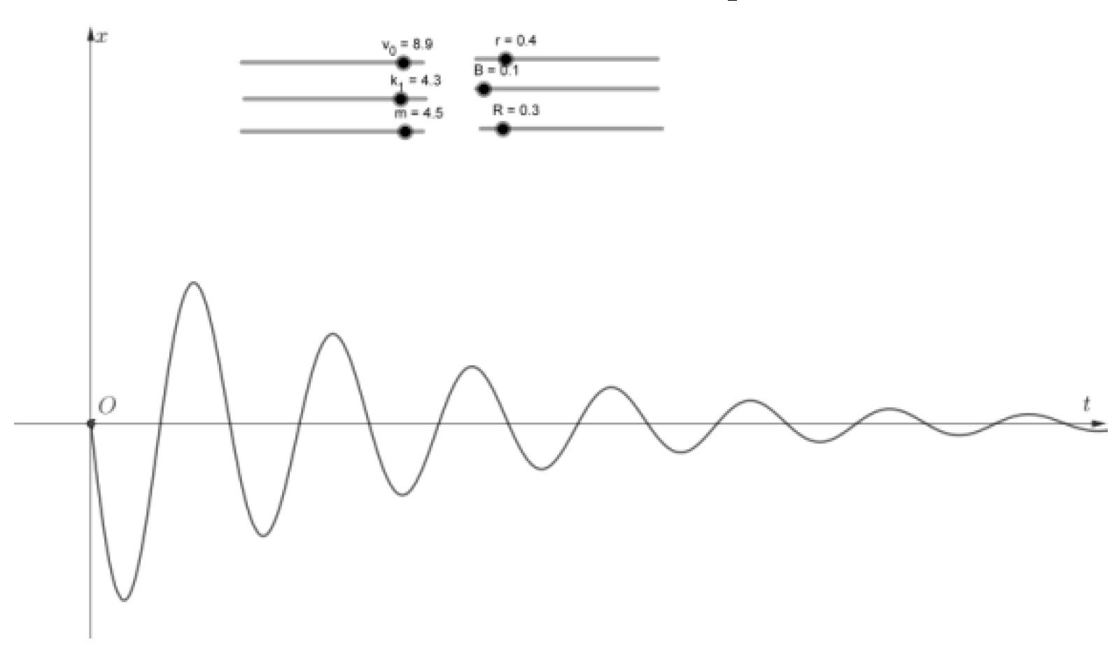
x = - \frac{v_{0}}{\sqrt{\frac{k_{1}}{m} - \frac{36 π^{4} r^{4} B^{4}}{m^{2} R^{2}}}} e^{- \frac{6 π^{2} r^{2} B^{2}}{m R} t} \sin (\sqrt{\frac{k_{1}}{m} - \frac{36 π^{4} r^{4} B^{4}}{m^{2} R^{2}}} t)

2.2. GeoGebra Visualization Process

(1) Create a slider v₀ and set the interval to (0,10), which suggests that the size of the initial velocity v₀ varies from 0 to 10 m/s; create a slider k₁ and set the interval to (0,5), which indicates that the spring strength coefficient k1 varies from 0 to 5 N/m; create a slider m and set the interval to (0,5), which suggests that the total mass of the platform and the three coils are m varies from 0 to 5 kg Create a slider r, set the interval to (0,2.5), which indicates that the radius r of each coil in the damping system varies from 0 to 2.5 m. Create a slider B, and set the interval to (0,2.5), which indicates that the magnitude of the magnetic induction B of the radial field where the coils are located in the damping system varies from 0 to 2.5 T. Create a slider R, set the interval to (0,2.5), which indicates that the magnitude of the magnetic induction B of the radiation field where the coils are located in the damping system varies from 0 to 2.5 T. R, set the interval as (0,2.5), indicating that the size of the resistance R of each coil in the damping system varies in the interval range of 0~2.5 Ω.

(2) Construct a specific function y of displacement over time for damped vibration (the pairwise relationship with the variables in the original functional equation is that t in the original equation corresponds to the present x, and x in the original equation corresponds to the present y), and enter y=if[x>=0,(-v_0)/sqrt(k_1/m-(36pi^4 r^4 B^4)/(m^2 R ^2))*e^((-(6pi^2 r^2 B^2))/(mR)*x)*sin(sqrt(k_1/m-(36pi^4 r^4 B^4)/(m^2 R^2))*x)] (NOTE: Type with “_” for subscript, “^ “ for superscript, “pi” for the constant π, and “if[x>=0,]” for the function’s domain of definition as x≥0)

At this point, the simulation model has been constructed. To display the variables corresponding to the horizontal and vertical coordinates, we need to create two “texts” and input “x” and “t” respectively with the checkbox “Latex formula” checked. Processed after moving to the end of the two axes at the end of the arrow, the effect is shown in Figure 4.

2.3. Python Visualization Process

The code used for visualization is following:

import matplotlib.pyplot as plt #import the package for graphing
import math #import frequently-used math functions
r=0.4;B=0.1;R=0.3;m=4.5;k1=4.3;v0=8.9;points=[] #set the parameters for visualization
for x in range(0,100,1): #generate points for accurate lining
y=(-v0)/math.sqrt(k1/m-(36*(math.pi**4)*(r**4)*(B**4))/((m**2)*(R**2)))*2.71828**((-(6*(math.pi**2)*(r**2)*(B**2)))/(m*R)*x)*math.sin(math.sqrt(k1/m-(36*(math.pi**4)*(r**4)*(B**4))/((m**2)*(R**2)))*x) #relation between x and t
points.append(y) #store the ‘x’ sets
plt.plot([i for i in range(0,100,1)],points)
plt.xlabel('t')
plt.ylabel('x')
plt.show() #graphing for visualization
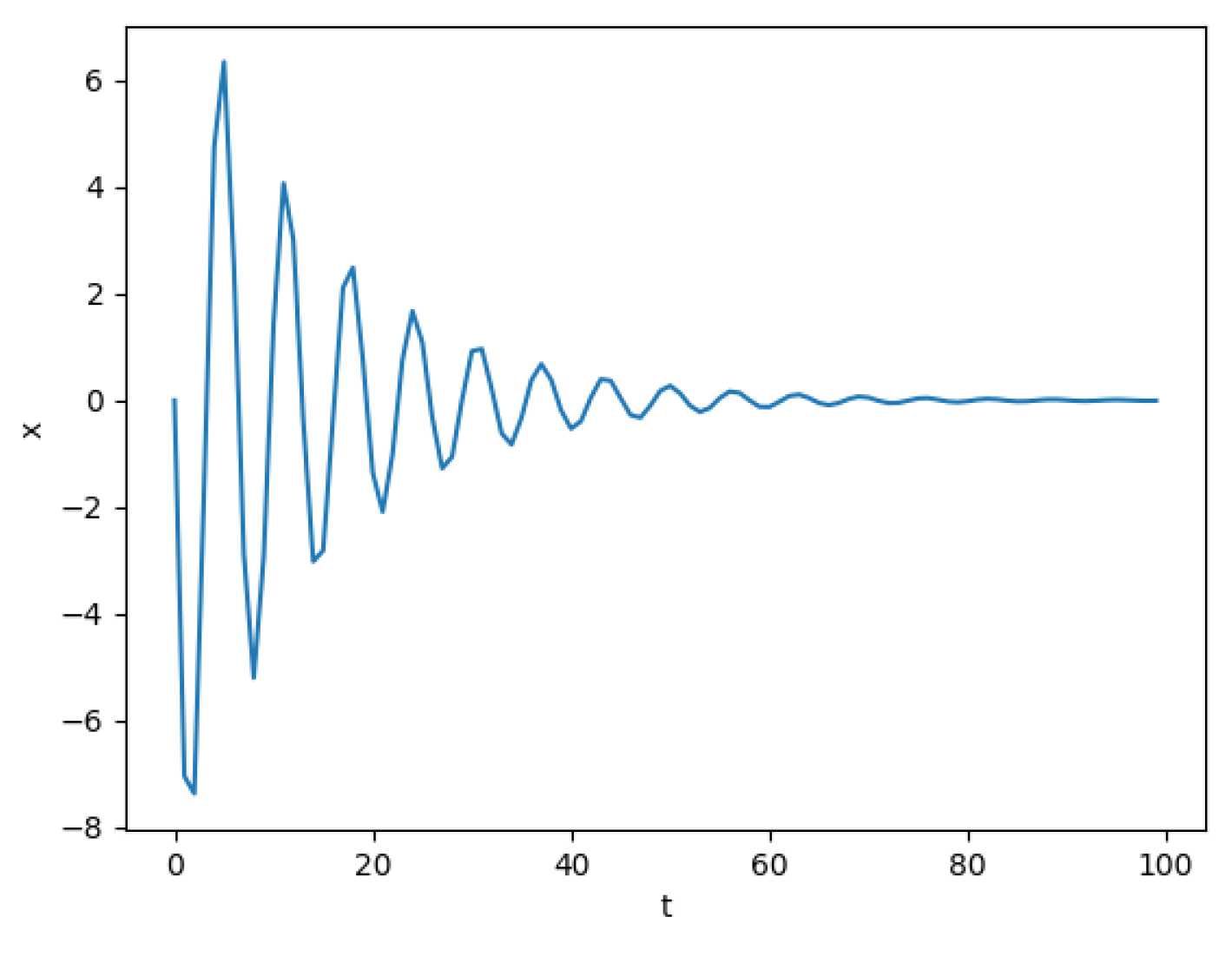
The result of Python visualization is shown in Figure 5.

3. Analysis of Visualization Results

(1) Based on the visualization depicted in Figure 5, it is evident that the variable x demonstrates an approximate periodic behavior with respect to time t, suggesting that the damper system, considered holistically, continues to oscillate in proximity to the equilibrium position. Nonetheless, the amplitude of these oscillations undergoes a gradual diminution over time, owing to the dissipation of energy stemming from resistive forces. As the amplitude (and, by extension, the velocity) undergoes a decrement, the rate of energy dissipation mediated by drag forces experiences a commensurate deceleration, ultimately resulting in a diminished rate of amplitude decay as time progresses.[3].

(2) The damped vibration image involved in the title image is not a good fit with this model under any parameters, and can be closely and highly sensitively affected and determined by the spring stiffness coefficient k₁, the initial velocity v₀, the total mass of the platform and the three coils of m, the magnetic induction intensity B of the radial magnetic field where the coils are located in the vibration-damping system, the resistance of each coil in the vibration-damping system, R, and the radius of each coil in the vibration-damping system, r, and so on. The parameters are influenced and determined. An example is given.

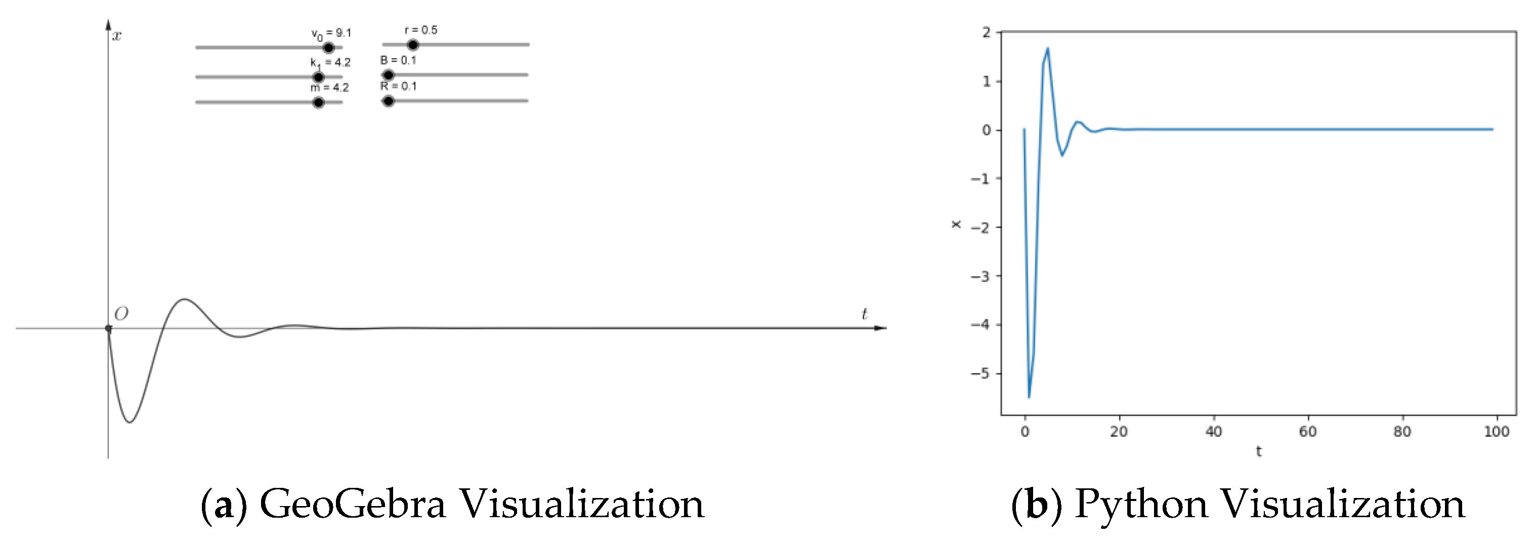
Each parameter takes the following values: v₀ =9.1 m/s, k₁ =4.2 N/m, m=4.2 kg, B=0.1 T, R=0.1 Ω, the software process finds that r is only in a small range of 0~0.6 m. The graph line can be closely adapted to the situation shown in Figure 5. When r is too large, the situation is shown in Figure 6(a) and Figure 6(b).

4. Comparison of Two Methods in Visualization

At the beginning, I employed GeoGebra software to delve into the precise functional relationship between displacement and the temporal evolution within a damping system. This system is influenced by the elasticity of springs, gravitational forces, and amperometric resistance during its damping motion. I have delineated several typical parameter ranges, illustrative images, and distinctive parameter scenarios that correspond to the problematic imagery. These elements collectively facilitate the comprehensive visualization of the dynamic progression of the physical model, thereby enhancing the comprehension of both students and educators regarding the underlying physical laws and the intricacies of the subject matter.

And either,then,I used Python for visualization.Python’s strength lies in its ability to handle large datasets and to integrate with other data analysis tools. However, it requires a certain level of programming knowledge and can be overkill for simple visualization tasks,while students and teachers possibly do not have the knowledge that supports the visualization process in Python.Also,visualization results generated using Python can sometimes appear less smooth when the number of manually controlled sampling points is insufficient. This limitation arises because the quality and smoothness of a visualization are highly dependent on the density and distribution of the data points. With fewer sampling points, the visual representation may not accurately capture the underlying patterns or trends in the data. Additionally, the lack of sufficient sampling points can lead to jagged or discontinuous lines in plots, which can be misleading or difficult to interpret,which might confuse the thinking of students. Furthermore, this issue can also affect the ability to interact with the visualization in real-time. Real-time interaction typically requires a dynamic and responsive system that can update the visualization as the user manipulates the data or explores different aspects of the visualization. When the data is sparse or the sampling points are not optimally distributed, the system may struggle to provide a seamless and responsive user experience. This can result in delays or inaccuracies in the visualization updates, which can hinder the user’s ability to explore the data effectively and make informed decisions based on the visual insights.

Apparently, GeoGebra is an interactive geometry, algebra, statistics, and calculus application that is user-friendly and widely used in educational settings. It provides an intuitive graphical interface for plotting functions, which is particularly beneficial for students and educators. GeoGebra excels in its ease of use and immediate visual feedback, making it ideal for exploring mathematical concepts in real-time. Nonetheless, it may lack the advanced customization and scalability options that Python offers, particularly when dealing with more sophisticated or data-intensive visualizations.

In essence, Python is a powerful tool for those who require extensive control and customization in their visualizations, while GeoGebra is a more accessible and interactive option for educational purposes and quick, straightforward visualizations.So,In conclusion,students who are interested in or master Python might be suitable persons for customization and their peers might actually be suitable for interactive visualization in classes.

5. Conclusion and Expectation

In the evolving landscape of education, where the complexity and application of mathematical concepts are increasingly emphasized, the choice of tools for visualization plays a critical role. Python, with its extensive control and customization capabilities, is ideal for students who are tech-savvy or have a strong grasp of programming. It enables them to delve deeper into the intricacies of mathematical functions and data analysis, allowing for a more nuanced understanding and manipulation of complex visualizations. Conversely, GeoGebra, with its user-friendly interface and interactive capabilities, serves as an excellent educational tool for those who prefer a more intuitive approach to visualizing mathematical concepts. Its dynamic and adjustable features make it particularly effective in illustrating the principles of motion and vibration-damping devices, which can be challenging to grasp conceptually.

The mixture of such tools in the classroom can cater to a diverse range of learning styles and preferences, thereby enhancing the educational experience. As students navigate the complexities of advanced mathematical concepts, the availability of both Python and GeoGebra provides a comprehensive toolkit that can help them adapt to the “new context, strong application, comprehensive and variant” challenges posed by educational reforms. This approach not only aids in the understanding of abstract mathematical laws but also prepares students for the real-world applications of these principles, thereby bridging the gap between theoretical knowledge and practical skills.

References

Jan Fiala; Projectile Motion: More Geometry, More Physics. Phys. Teach. 2024, 62, 210–213. [CrossRef]
Walsh, T. Creating interactive physics simulations using the power of GeoGebra. Phys. Teach.
Zheng YL,Jia QM,Fang SM. Mechanics [M].3 ed. Beijing: Higher Education Press 2018, 298-299.

Figure 4. GeoGebra visualization result.

Figure 5. Python visualization result.

Figure 6. Typical image when r is too large.

Disclaimer/Publisher’s Note: The statements, opinions and data contained in all publications are solely those of the individual author(s) and contributor(s) and not of MDPI and/or the editor(s). MDPI and/or the editor(s) disclaim responsibility for any injury to people or property resulting from any ideas, methods, instructions or products referred to in the content.

© 2024 by the authors. Licensee MDPI, Basel, Switzerland. This article is an open access article distributed under the terms and conditions of the Creative Commons Attribution (CC BY) license (https://creativecommons.org/licenses/by/4.0/).

Copyright: This open access article is published under a Creative Commons CC BY 4.0 license, which permit the free download, distribution, and reuse, provided that the author and preprint are cited in any reuse.

MDPI Initiatives

Important Links

Choose an area of interest and we will send you notifications of new preprints at your preferred frequency.

Disclaimer

Comparison of Using GeoGebra and Python to Discover the Motion of Device in a Well-Known Physical Experimental Instrument—Looking into Vibration-Damping Devices in the Scanning Tunneling Microscope

Abstract

1. Presentation of the question after modeling

2. Analytical Modeling and the Visualization of GeoGebra and Python

2.1. Theoretical Modeling Process

2.2. GeoGebra Visualization Process

2.3. Python Visualization Process

3. Analysis of Visualization Results

4. Comparison of Two Methods in Visualization

5. Conclusion and Expectation

References

MDPI Initiatives

Important Links

Subscribe