2.1. The Phenomenological Model
In [
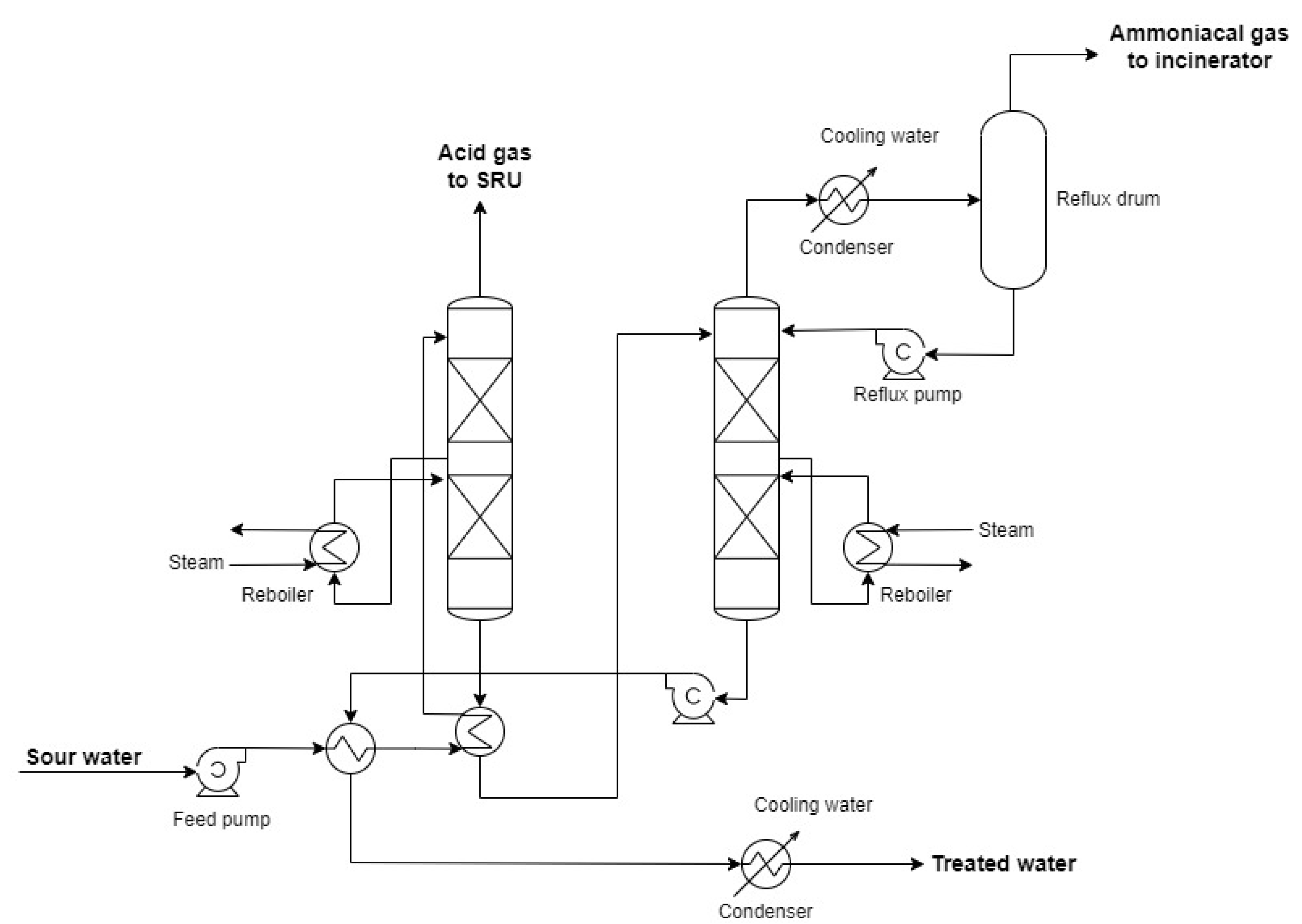
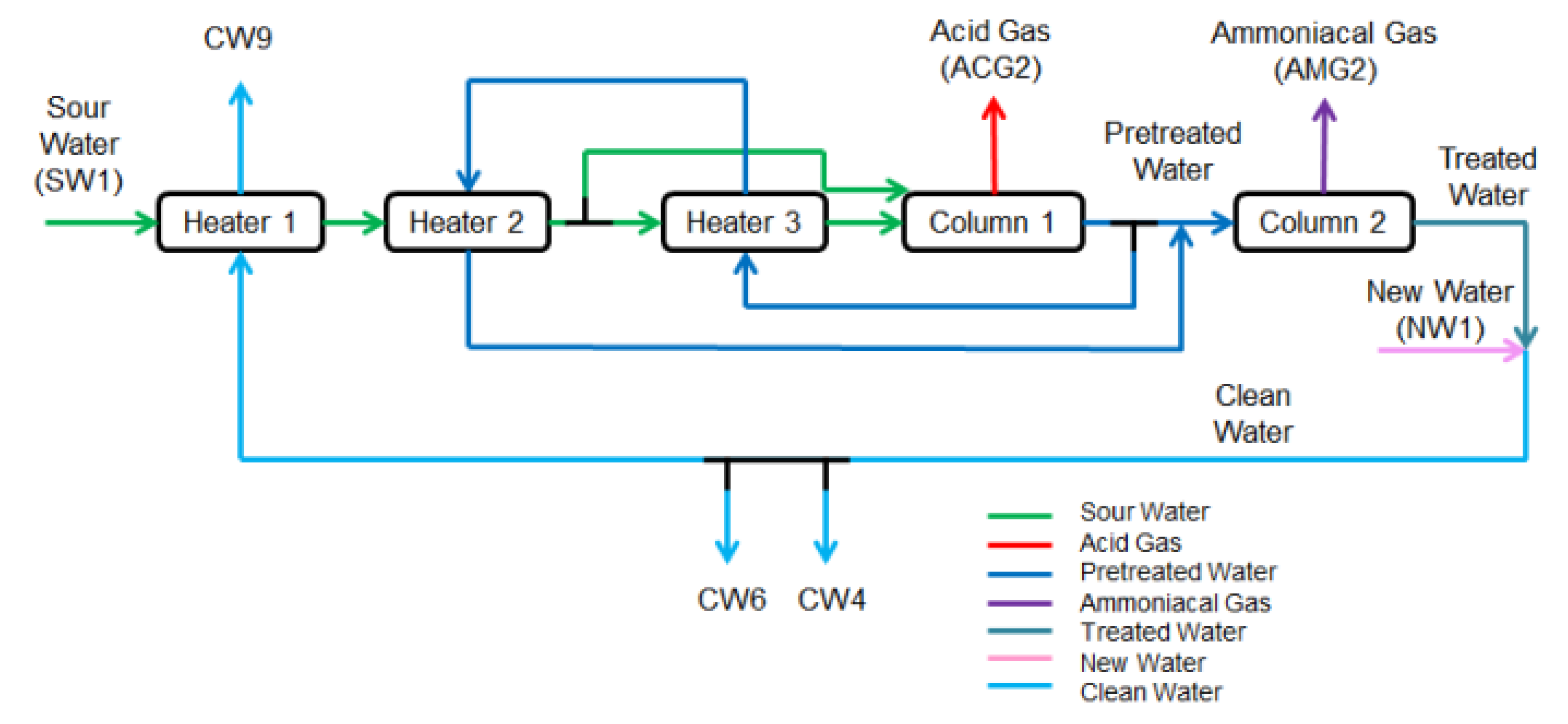
1], the author conducted the dynamic simulation of a SWTU in Aspen Plus Dynamics® V10 using the Gas Process Association Sour Water Equilibrium (GPSWAT) model, considered the most suitable for sour water applications. In this simulation, there are thirty-four material streams and seven different compositions, three heat streams, and twenty-three pieces of equipment: twelve valves, three heat exchangers, three splitters, two mixers, one pump, and two columns. The block diagram in
Figure 2 summarizes all the streams and key equipment in the simulation, where H1, H2, and H3 are the heat exchangers, and C1 and C2 are the stripping columns.
The seven different compositions described in the process are sour water, which is the incoming stream to be treated; acid gas, which is the overhead stream from the first column rich in H₂S; ammoniacal gas, which is the overhead stream from the second column rich in NH₃; pre-treated water, which is the bottom stream from the first column, hence rich in NH₃; treated water, which is the bottom stream from the second column, containing small amounts of dissolved H₂S and NH₃ contaminants; new water, which is an aqueous stream without contaminants, and finally, clean water, which is the mixture of new water with treated water.
Table 1 correlates the abbreviations of these streams with their compositions.
The two input streams of the process are SW1 and NW1, while the five output streams are ACG2, AMG2, CW4, CW6, and CW9. SW1 is the sour water to be treated, and NW1 is the new uncontaminated water source that dilutes the treated water stream after passing through the two columns.
Table 2 displays the physical properties of the input streams.
These streams had their mass flow described as a function of SW1, defined as SW1F. These values were anonymized due to the confidentiality of information that originated the simulations developed by [
1].
Finally, ACG2 and AMG2 are the outputs of acid gas and ammoniacal gas, respectively. CW4, CW6, and CW9 are the outputs of clean water with the same composition.
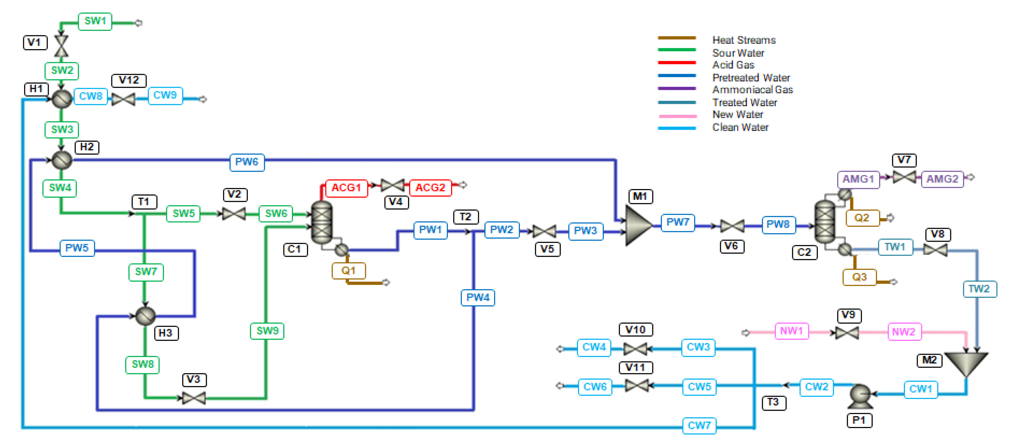
The simulation begins with the SW1 stream, which is preheated in heat exchangers H1 and H2 through energy integration with streams CW7 and PW5, respectively, becoming SW4. SW4 is divided into SW5 and SW7. SW5 becomes SW6 after passing through valve V2 and enters the top of column C1. SW7 is preheated once again in heat exchanger H3 through energy integration with PW4 and becomes SW9 after passing through valve V3, subsequently entering the lower feed of column C1. Therefore, streams SW6 and SW9 feed C1.
Column C1 is heated by the thermal load Q1 from the reboiler, separating the overhead stream ACG1 (acid gas) from the bottom stream PW1 (pre-treated water). ACG1, after valve V4, becomes ACG2 and is removed from the system, while PW1 is split into two streams: PW2 and PW4. PW4 is cooled in heat exchanger H3 through energy integration with SW7 and becomes PW5. PW5 is further cooled in H2 through energy integration with SW3 and becomes PW6. PW2 becomes PW3 after passing through valve V5 and is mixed with PW6, forming PW7. It is noteworthy that PW7 has the same mass flow as PW1, as the streams that split reunite without losses. After valve V6, PW7 becomes PW8 and enters the feed of column C2.
Column C2 has a condenser and a reboiler, with thermal loads Q2 and Q3, respectively. The overhead stream from Column 2 is AMG1 (ammoniacal gas), and the bottom stream is TW1 (treated water). AMG1, after valve V7, becomes AMG2 and is removed from the system. TW1, after valve V8, becomes TW2. TW2 is mixed with NW2, becoming clean water (CW1). After passing through pump P1, CW1 is then called CW2. CW2 is divided into three streams: CW3, CW5, and CW7. CW3, after valve V10, becomes CW4 and is removed from the system. CW5, after passing through valve V11, becomes CW6 and is removed from the system. Meanwhile, CW7 is cooled in heat exchanger H1 through energy integration with SW2, becoming CW8. CW8, after valve V12, becomes CW9 and is removed from the system. A more complete view of the process is in
Figure 3, showing the static simulation developed by [
1].
There are two 'RadFrac' type columns and three 'HeatX' type heat exchangers in the simulation. Column C1 consists of 5 stages, and Column C2 consists of 6 stages. The feed occurs at stages 1 (SW6) and 2 (SW9) in C1, and at stage 2 (PW8) in C2. The two mixers were configured to receive both liquid and vapor phases. Valves V4 and V7 were configured only to receive vapor, while the other valves accept only the liquid phase. All valves have an associated pressure drop.
The dynamic model by [
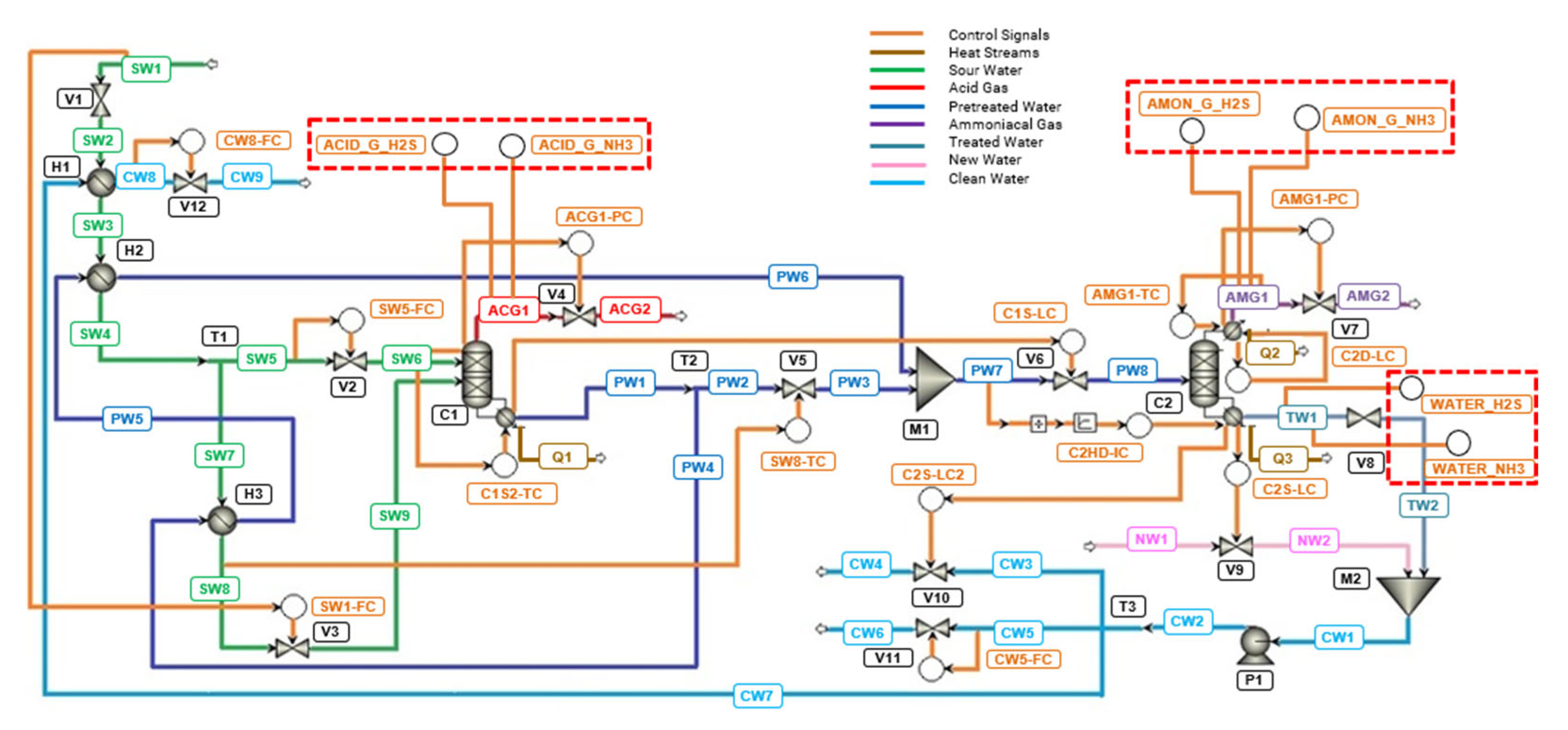
1] includes 14 controllers added to ensure the operability and stability of the process, as well as aid in the convergence of the dynamic simulation. The controllers in the simulation are: two for pressure at the tops of the columns, four for level at the bottom and top of the columns, three for temperature, including one before the first column and one in its second stage, and another at the top of the second column; four mass flow controllers, two before the first column and two after the second column; and an integrated control of mass flow and thermal load in the second column.
Table 3 describes the controlled and manipulated variables for each of these controllers.
The tuning of the controllers was performed based on general rules described in the literature and through expert advice from the industry [
1].
The first step in creating the new database for the development of soft sensors involved the inclusion of six controllers not previously used in the dynamic simulation of the SWTU with two stripping columns by [
1].
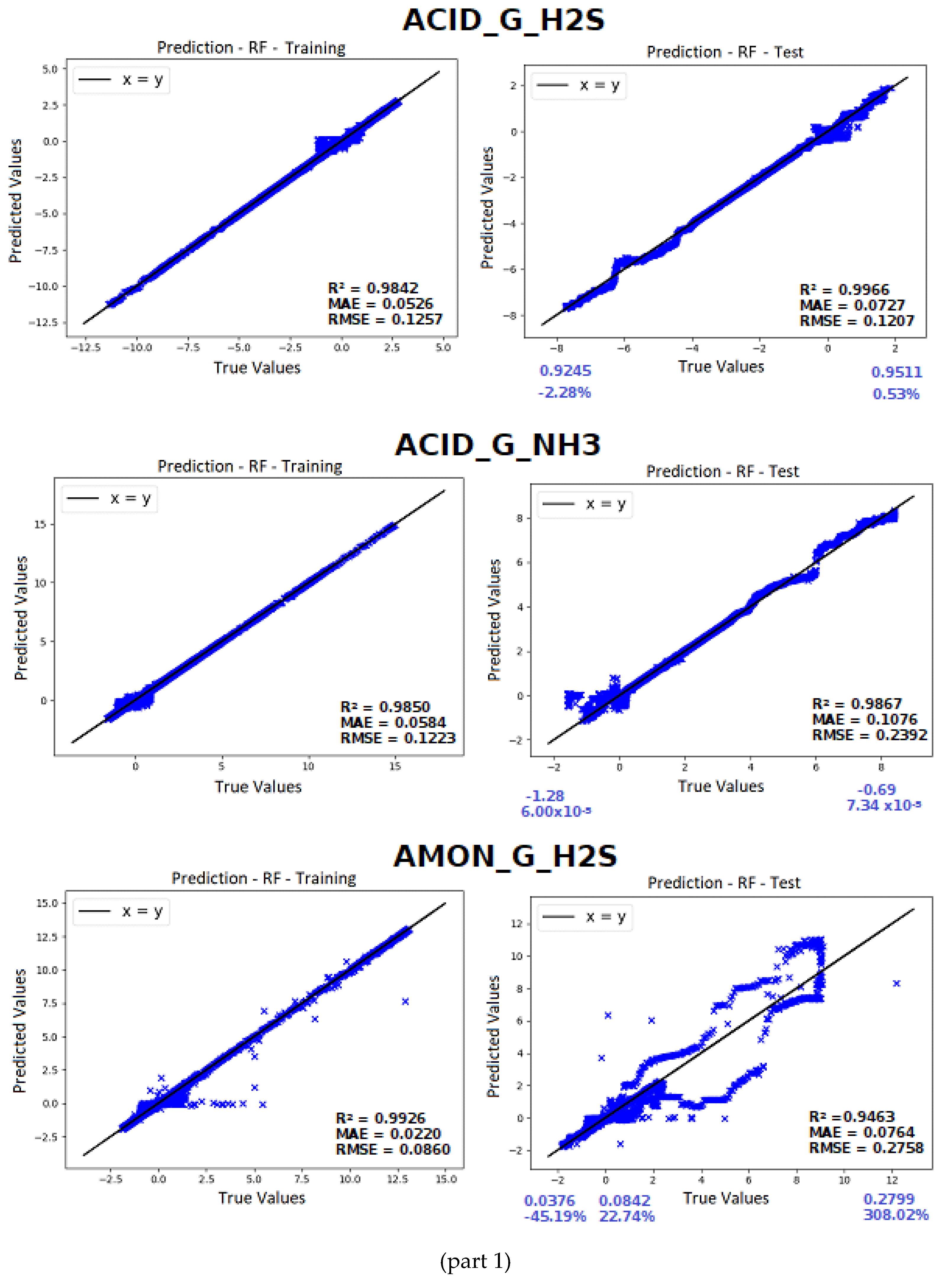
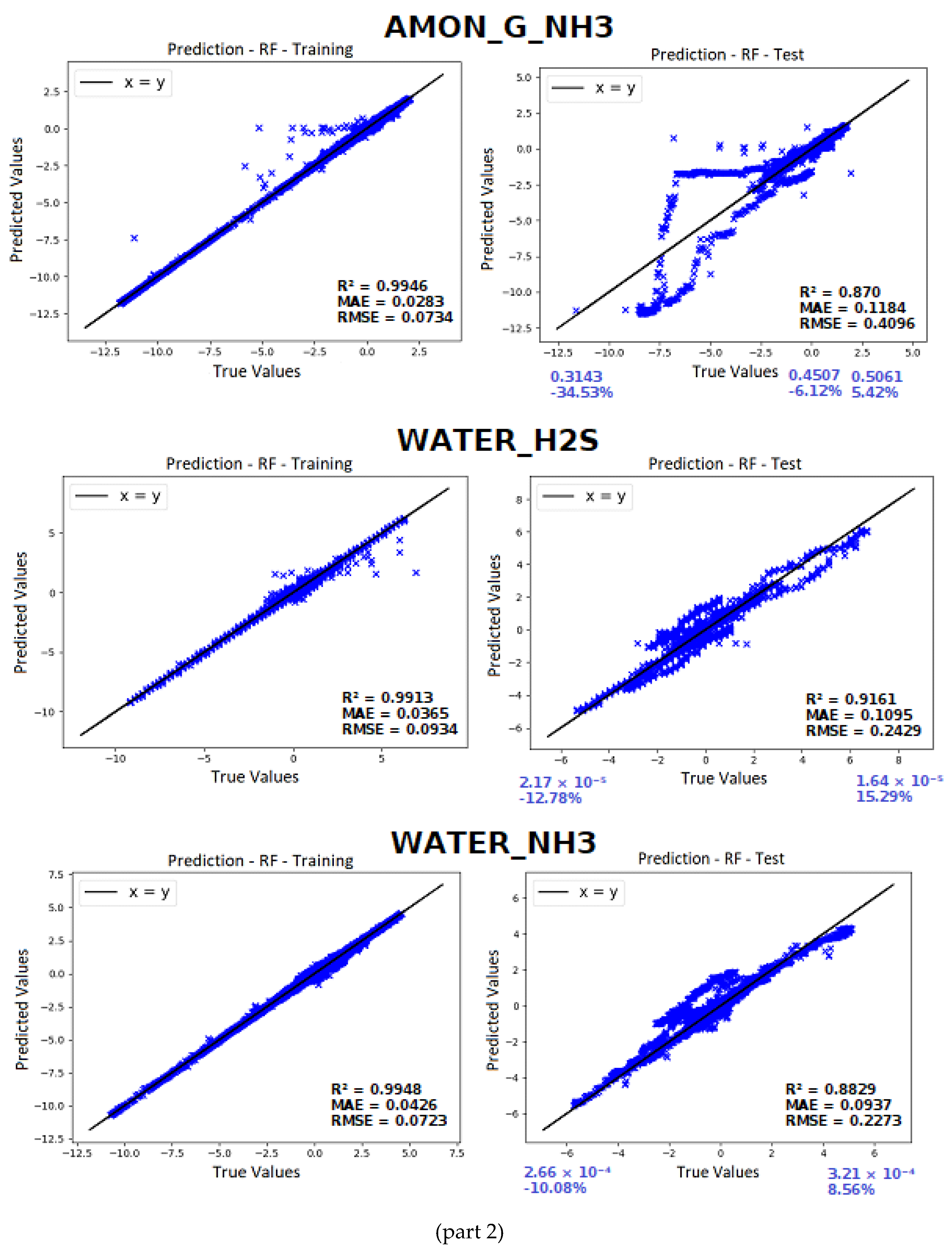
Among these controllers, two were incorporated into the acid gas stream (ACG1) at the top of Column 1 (ACID_G_H₂S and ACID_G_NH₃), another two were added to the ammoniacal gas stream (AMG1) at the top of Column 2 (AMON_G_H₂S and AMON_G_NH₃), and two more (WATER_H₂S and WATER_NH₃) were introduced into the treated water stream (TW1) withdrawn from the bottom of Column 2. The six new controllers can be seen in
Figure 4, along with the original simulation controllers.
To enable the collection of dynamic data for the fractions of H₂S and NH₃ in the effluents described, the PID (Proportional, Integral, Derivative) controllers included were adjusted with a gain of 0, an integral time of 1 minute, and a derivative time of 0. This configured them to operate solely as 'indicators', without effectively performing control functions during the simulation, only storing the dynamic data.
2.2. Development of the Database and Phenomenological Study of the Process
The simulations, calculations, and codes were developed and executed on a computer with an Intel(R) Core™ i5 7200U, with a CPU@ 2.50 GHz 2.70 GHz processor, 8.00 GB installed memory (RAM), and Windows 10 64-bit operating system. The dynamic simulation of the SWTU was performed using Aspen Plus Dynamics® V10. All data processing and Artificial Intelligence algorithms were implemented in Python 3.11.4 within the integrated development environment Visual Studio Code 1.79.2. The libraries numpy (1.25.2), matplotlib (2.0.2), joblib (1.3.2), scikit-learn (0.19.0), pandas (2.1.0), seaborn (0.12.2), and optuna (3.3.0) were extensively used.
The dynamic simulation, after the changes discussed in
Section 2 and illustrated in
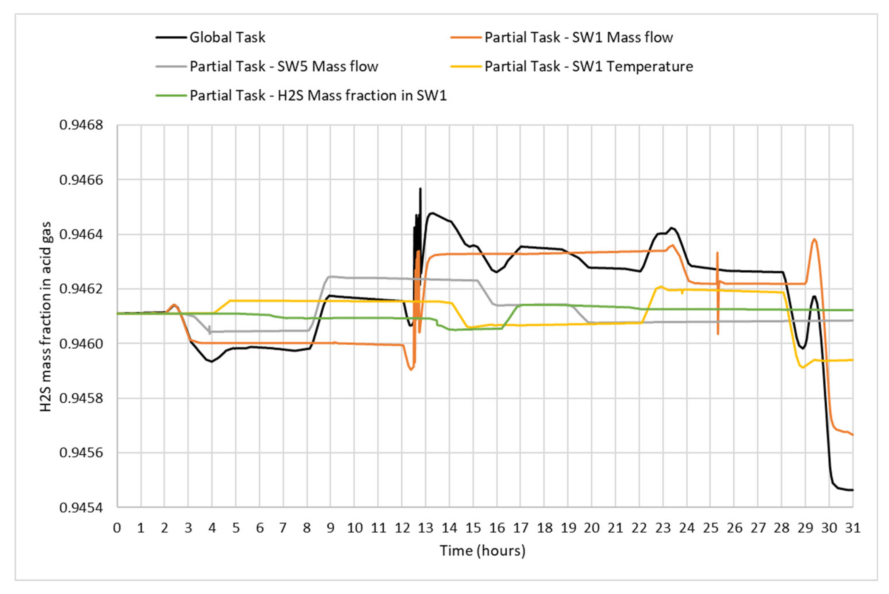
Figure 4, was tested in various scenarios of normal operation with disturbances in five variables of interest, namely, SW1 mass flow rate, SW5 mass flow rate, SW1 temperature, and NH₃ and H₂S mass fractions in SW1. These variables were chosen because they are input process variables that could undergo variations in a real process. SW1 is the sour water entering the system for treatment, and SW5 represents 10% of SW1, which, after passing through the heat exchangers, enters the top of column C1. Normal operation is characterized when events such as complete valve opening or closing, overflows, or lack of level in the columns do not occur.
2.3. Comparison of Artificial Intelligence Algorithms
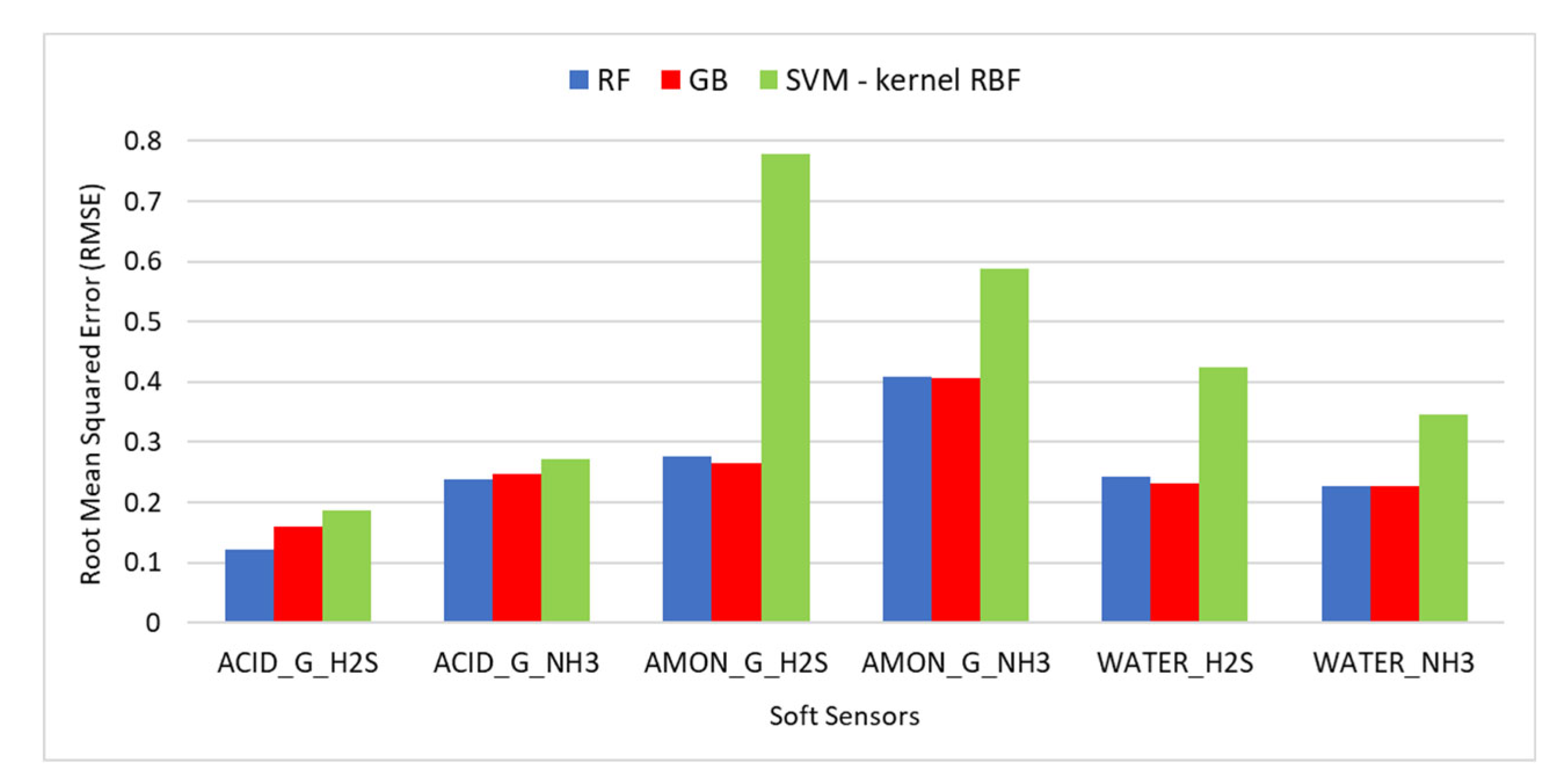
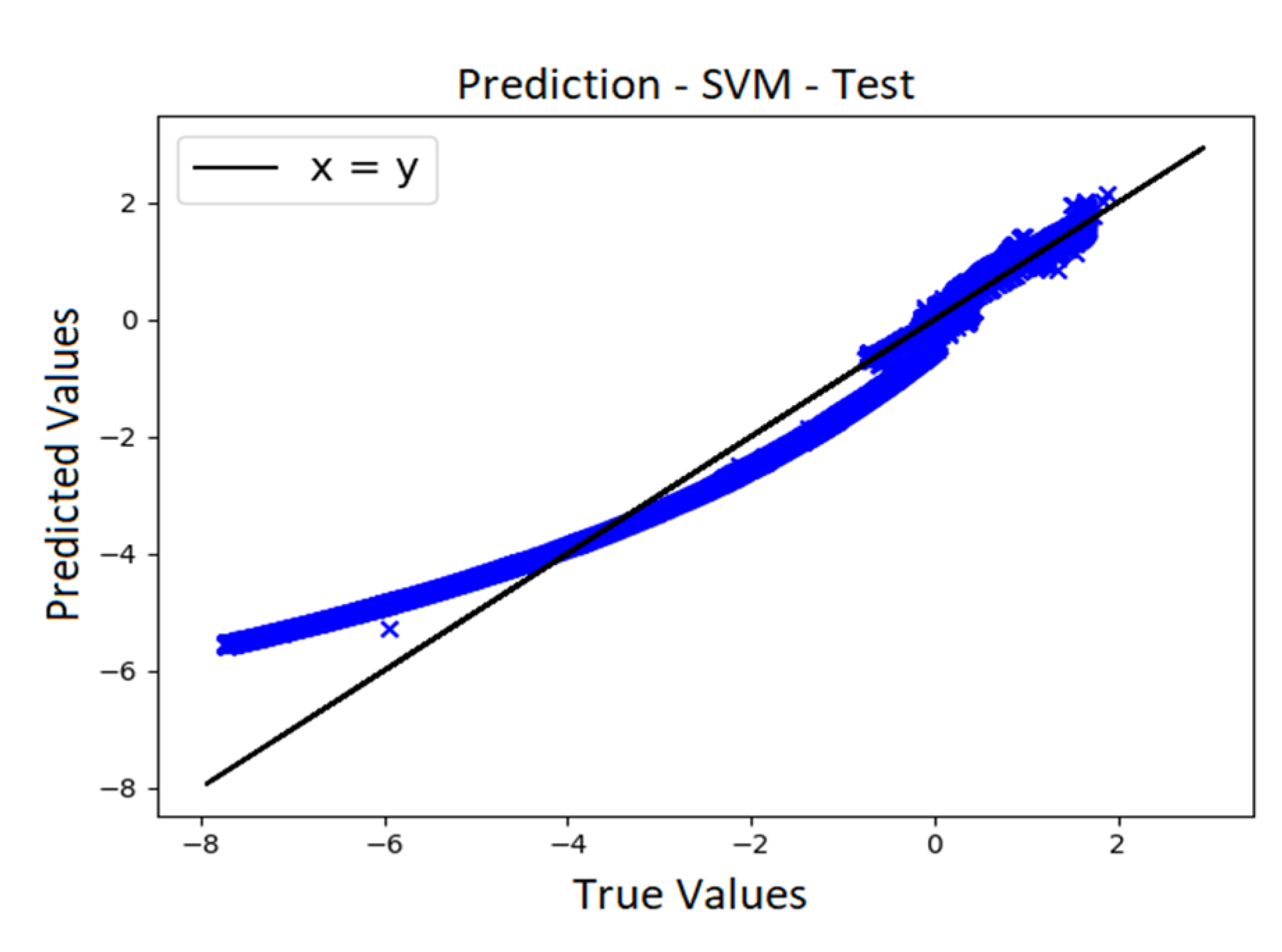
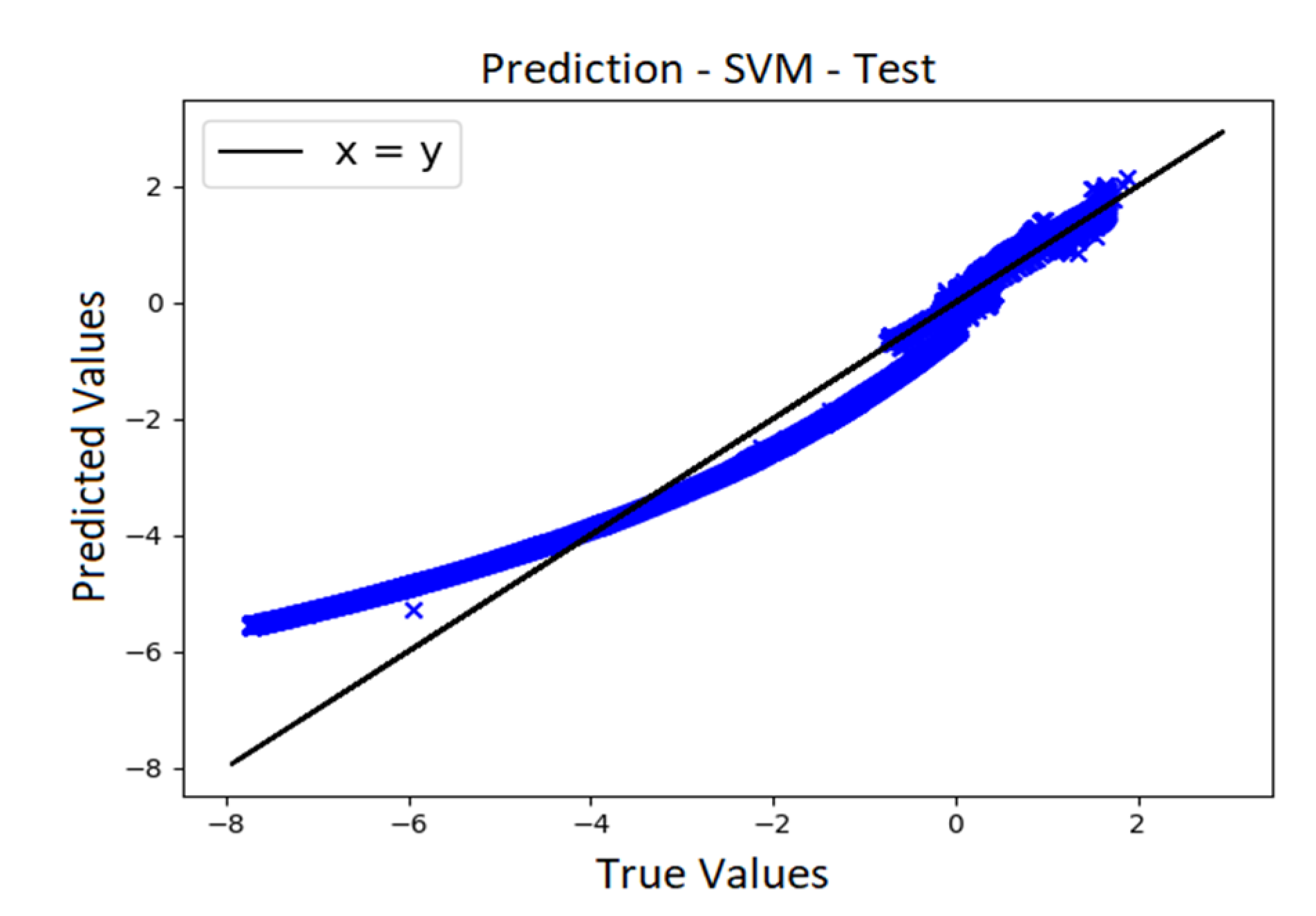
To create the six soft sensors, AI tools such as Random Forests, Gradient Boosting, and SVM with linear and RBF kernels models were evaluated using the same training and test datasets. The methods of Gradient Boosting (GradientBoostingRegressor function), Random Forest (RandomForestRegressor) and SVM (SVR function, linear and RBF kernels) from the scikit-learn library (version 0.19.0) were employed. These kernels were chosen because they demonstrated the best results and the shortest computational times in a previous study [
24].
Optuna library was used for hyperparameter optimization of the RF algorithm, aiming to obtain the most effective and accurate model for each of the six sensors. The optimized hyperparameters included the number of estimators (rf_n_estimators), representing the number of trees in the forest, the maximum depth of the trees (rf_max_depth), and the minimum number of samples required to form a leaf (terminal node) of the tree (rf_min_samples_leaf). The lower and upper limits were defined for each of the RF hyperparameters and are shown in
Table 4. This methodology enhances the efficiency of the optimization by eliminating the need to consider extreme or impractical values and helps to prevent overfitting or underfitting issues in the model and resulting in computational time savings. Similarly, the number of iterations (or number of trials) for the hyperparameter optimization process was set to 40.
Analogously to the RF, the same hyperparameters mentioned in
Table 4 were optimized for the GB algorithm using the same limits and number of iterations, while for the SVM models, there was no optimization of the hyperparameters (C and gamma), as optimizing them did not yield significant gains as shown by [
24].
Data processing takes place after storing the dynamic data from all 20 controllers after each simulation (or simply 'run'). Concatenating this information within normal operation resulted in the development of the database, which was later divided into training and testing data to be used in the development of AI-based soft sensors. To guarantee the representativeness and efficient training of the models, it was ensured that each database had at least one example of each simulation in normal operation. Additionally, all data related to a single run were consolidated in the same database to prevent data leakage, especially considering that the simulations contain temporal data. Furthermore, data shuffling, separation into inputs and outputs, as well as normalization were performed.
After dividing the database, the training set consisted of 45,483 samples (59%), while the test set contained 31,525 samples (41%). The listing with the description of each simulation that composed each set can be found in
Table 5 and
Table 6.
To clarify the division of runs between training and testing databases, each database contains one example of each simulation. Although they share the same description, each simulation is unique, featuring various versions in terms of intensity, amplitude, and timing of the disturbances. The normalized database can be found in [
29].
2.6. Implementation to a real SWTU
In this section the knowledge gained with the approach based on the phenomenological model is employed to develop random forest models using data from a real SWTU of a Brazilian oil refinery. The chosen unit for this development has the same flowsheet configuration of the simulated plant, making it possible to use the same inputs as in the simulated modelling.
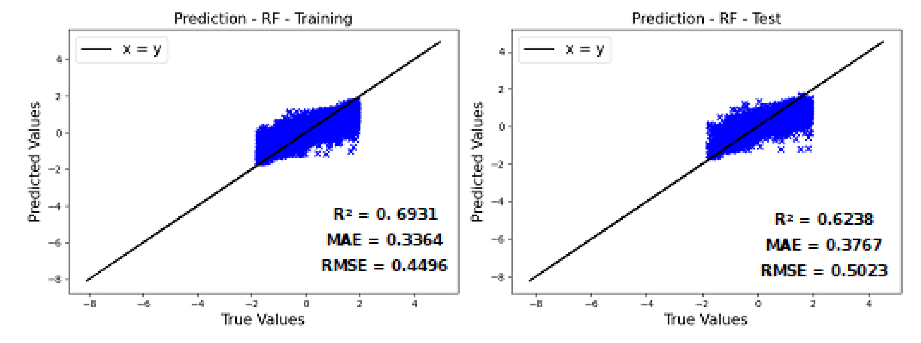
The WATER_NH₃ sensor was selected for modeling. For this sensor, the plant utilizes an online analyzer that produces results approximately every 20 minutes. Unfortunately, analysis for acid and ammoniacal gases were not conducted on the site and only a limited number of laboratory results were available for H₂S on treated water. This was expected due to the hazards involved in sampling acid gas and that H₂S is not a primary concern on treated water given that H₂S is easier to remove than NH₃ in the second column, making more sense to control only the NH₃ content on treated water.
Even though the online analyzer generates results every 20 minutes, it is worth to mention that any control application to be implemented on the plant would need information at least on a minute basis, justifying the importance of modeling this kind of sensor even in a plant with online analyzer.
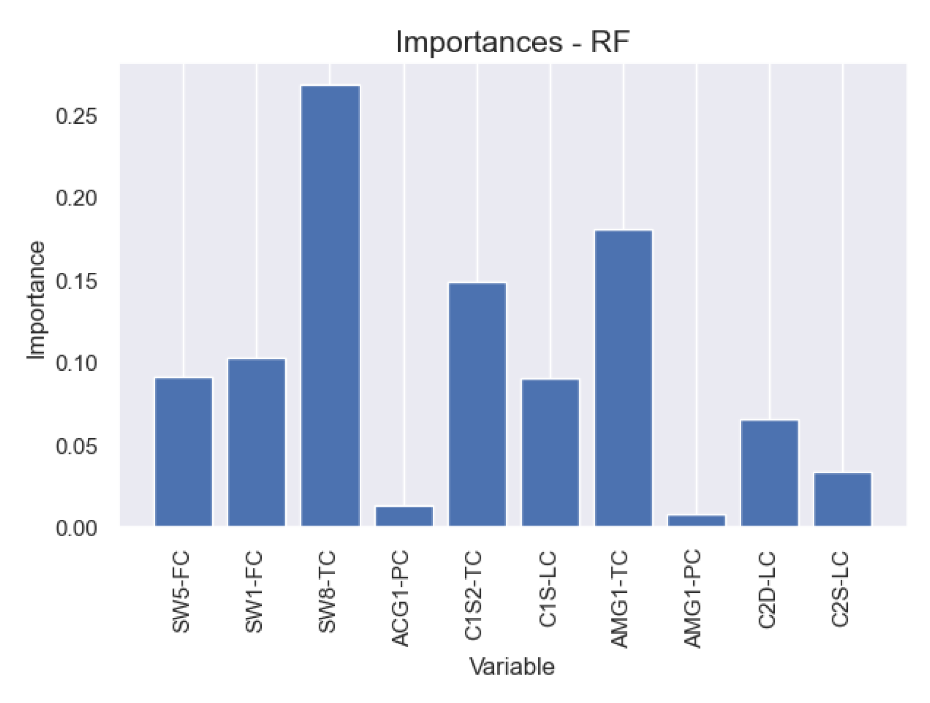
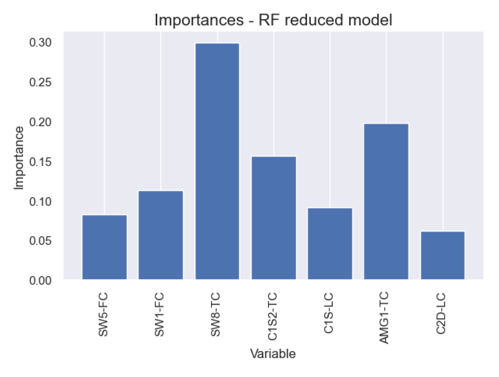
Given that operating conditions of the industrial plant did not precisely match the intervals used in the simulation runs, it was not prudent to use directly the models obtained with simulation data. Therefore, the sensor was retrained with real plant data. Variables SW5-FC, SW1-FC, SW8-TC, ACG1-PC, C1S2-TC, C1S-LC, AMG1-TC, AMG1-PC, C2D-LC, C2S-LC were considered as input variables. Variables CW8_FC, C2HD-IC, CW5-FC were not included as these measurements were not available in the real plant.
The first step of data acquisition involved retrieving results from the analyzer, starting from its installation date, covering a period of 22 months, yielding 40,338 results. Subsequently, rather than acquiring input data, at the same timestamps of the analyzer results, they were collected applying a 20-minute time average prior to those timestamps. This approach is due to the need to minimize not only the effects of dynamic and dead times but also disturbances characteristics of any industrial plant. It is believed that using the input values on exactly the timestamps of the analyzer results would not correctly represent the information that generated the outputs.
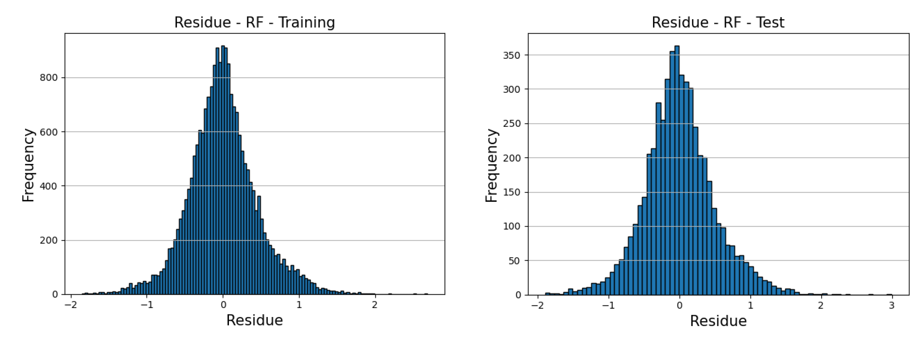
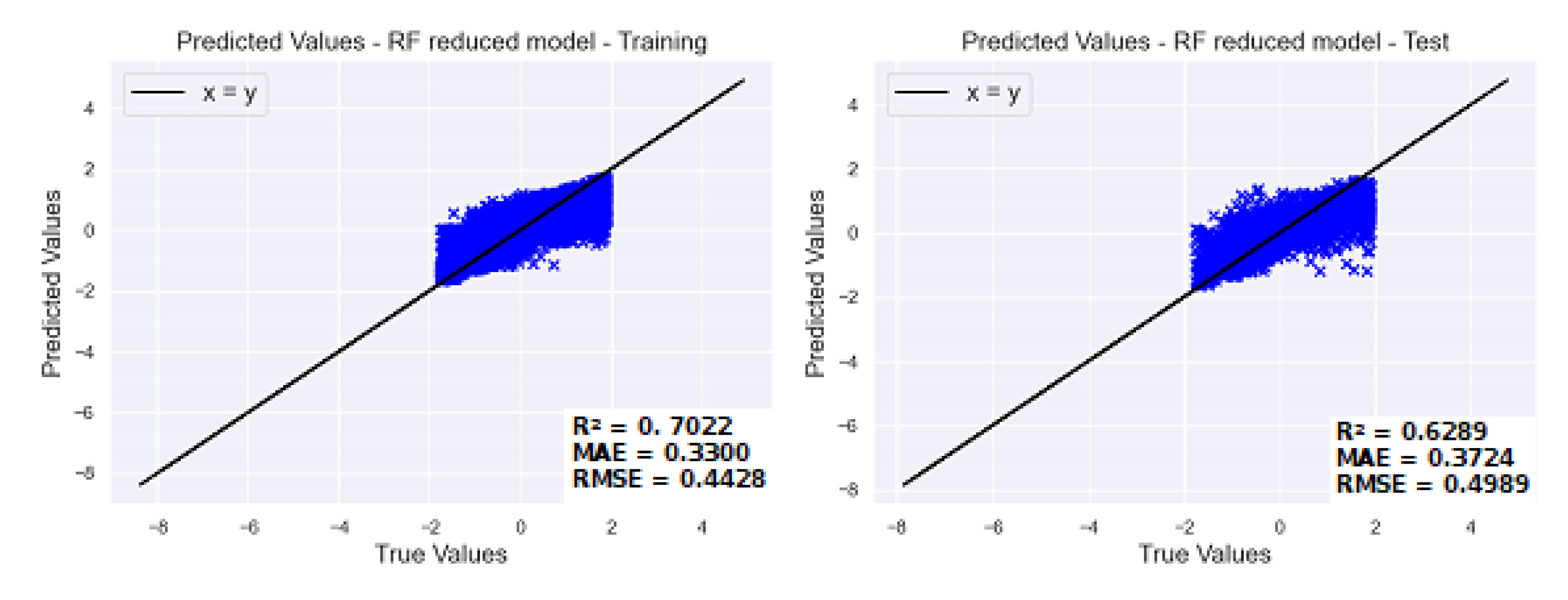
Before modelling, an interquartile range method was applied to remove outliers. The scale value used was 1.7, which means that this procedure discarded any value greater than 3 standard deviations from the respective mean. The final useful data were composed of 21,433 rows. The data were normalized using the method StandardScaler from python scikit-learn module. The normalized data were split into 10% for test and 90% for training from which 20% was reserved for validation.
Model training was executed with the same methodology used in training with simulated data, which consisted of using python’s Optuna library to explore the hyperparameters of Random Forest Regressor, i.e., rf_min_samples_leaf (1 to 10), rf_max_depth (5 to 10) and rf_n_estimators (1 to 50). The best model hyperparameters were, respectively, 1, 10 and 48.
