Preprint
Article

Gastric Cancer Detection with Ensemble Learning on digital pathology: Use Case of Gastric Cancer on GasHisSDB Dataset

Altmetrics

Downloads

133

Views

78

Comments

0

A peer-reviewed article of this preprint also exists.

Submitted:

01 August 2024

Posted:

06 August 2024

You are already at the latest version

Alerts
Abstract
Gastric cancer has become a serious worldwide health concern, emphasizing the cru-cial importance of early diagnosis measures to improve patient outcomes. While tradi-tional histological image analysis is regarded as the clinical gold standard, it is la-bor-intensive and manual. Recognizing this problem, there has been a rise in interest in using computer-aided diagnostics tools to help pathologists with their diagnostic ef-forts. In particular, deep learning (DL) has emerged as a promising solution in this sector. However, current DL models are still restricted in their ability to extract exten-sive visual characteristics for correct categorization. To tackle this limitation, this study proposes the use of ensemble models, which incorporate the capabilities of sev-eral deep learning architectures and use aggregate knowledge of many models to im-prove classification performance, allowing for more accurate and efficient gastric cancer detection. To see how well these proposed models performed, this study com-pared them to other works, all of which were based on the Gastric Histopathology Sub-size Images Database, a publicly available dataset for gastric cancer. This research demonstrated that the ensemble models achieved high detection accuracy across all sub-databases, with an average accuracy exceeding 99%. Specifically, ResNet50, VGGNet, and ResNet34 performed better than EfficientNet and VitNet. For the 80 × 80 pixel sub-database, ResNet34 exhibited an accuracy of approximately 93%, VGGNet achieved 94%, and the ensemble model excelled with 99%. In the 120 × 120 pixel sub-database, the ensemble model showed 99% accuracy, VGGNet 97%, and ResNet50 approximately 97%. For the 160 × 160 pixel sub-database, the ensemble model again achieved 99% accuracy, VGGNet 98%, ResNet50 98%, and EfficientNet 92%, high-lighting the ensemble model's superior performance across all resolutions. Overall, the ensemble model consistently provided an accuracy of 99% across the three sub-pixel categories. These findings showed that ensemble models may successfully detect criti-cal characteristics from smaller patches and achieve high performance. The findings will help pathologists diagnose gastric cancer using histopathological images, leading to earlier identification and higher patient survival rates.
Keywords: 
Subject: Medicine and Pharmacology  -   Pathology and Pathobiology

1. Introduction

The GI tract, spanning 25 feet from the oral cavity to the anus, transports ingested substances. The digestive process begins with the oesophagus and continues through the stomach and small intestines, extracting important nutrients. Waste is then eliminated through the colon and rectum. [1,2] Tumors in these organs often result from aberrant cell growth caused by DNA changes.[4] Mutations can be caused by a variety of reasons, including health conditions, genetics, lifestyle. The uncontrolled proliferation of malignant cells in the gastrointestinal system is caused by genetic, environmental, and lifestyle factors that interact. Common gastrointestinal (GI) cancers include Esophageal Cancer, Colorectal Cancer, Gastric Cancer, Bile Duct Cancer, Anal Cancer, Colon Cancer, Gallbladder Cancer, Pancreatic Cancer, Gastrointestinal Stromal Tumours, Liver Cancer, Rectal Cancer, Gastric Cancer, and Small Intestine Cancer. In 2020, gastric cancer was one of the top three most common cancers in 19 nations, with around 1.1 million cases reported (720,000 men, 370,000 females). Early identification of GI cancer aids in cancer treatment and reduces health-related complications.
Traditional approaches for identifying cancer include estimating body fat percentage and thereafter correlating it to cancer. Other methods include identifying common microbes associated with cancer in food. Another way is the use of Indocyanine Green (ICG) in gastrointestinal surgery, which is gaining popularity, particularly for lymph node diagnosis and operative field imaging [13,14].
However, pathologists must physically assess tissue samples, which is a tough, time-consuming, and subjective procedure. Moreover, different pathologists may provide different results, making the analysis susceptible to errors. The accuracy of histopathological analysis is heavily dependent on the pathologists' experience and knowledge, making the manual process susceptible to mistakes such as incorrect detection and diagnosis. Furthermore, a scarcity of pathologists creates significant delays in examining patient cases, potentially leading to late cancer discovery [15,16].
Various computer-aided detection (CAD) strategies have been investigated for the diagnosis of gastric cancer utilizing histopathological imaging. For more than 30 years, researchers have studied computer-aided diagnosis in gastroenterology, creating datasets from endoscopic images using various methodologies. The most widely researched issue is the identification of aberrant pathological signs in a specific location of the GI tract, notably polyps. There has also been research on detecting and categorizing disorders throughout the GI system, such as clinical findings, anatomical markers, and therapeutic therapies [3].

2. Materials and Methods

2.1. Literature Reviews

Various computer-aided detection (CAD) strategies have been investigated for the diagnosis of gastric cancer utilizing histopathological imaging. For more than 30 years, researchers have studied computer-aided diagnosis in gastroenterology, creating datasets from endoscopic images using various methodologies. The most widely researched issue is the identification of aberrant pathological signs in a specific location of the GI tract, notably polyps. There has also been research on detecting and categorizing disorders throughout the GI system, such as clinical findings, anatomical markers, and therapeutic therapies [3]. During the first 20 years of development, image processing required extracting features using various approaches and then categorizing them using statistical methods [19]. These characteristics were divided into three categories: spatial, frequency, and high-level descriptors. Spatial characteristics were retrieved using pixel-based and histogram techniques, whilst frequency information was collected using Fourier and wavelet transform algorithms. High-level characteristics were retrieved with edge and region-based methods. Statistical machine-learning approaches were frequently employed to categorize these characteristics.
Later, machine learning (ML) is commonly used in CAD to diagnose gastric cancer by extracting handmade elements such as color, texture, and form. For this purpose, support vector machines (SVM), random forests, and Adaboost are among the most frequently employed machine learning classifiers. In recent research, deep learning has been utilized to automate the feature selection process. Several studies have shown that deep convolutional neural networks (CNN) excel at tasks such as recognizing and segmenting histopathological images related to cancer, metastasis, and genetic mutation analysis. Some investigations have indicated that these networks perform similarly to human pathologists [7,8].
Deep learning techniques have advanced significantly over the past decade, notably with the CNN architecture. This design allows for the extraction and categorization of spatial as well as high-level features, making it a major area of study for academia. Several solutions have been proposed, including hybrid approaches based on CNN attributes, transfer learning, the development of novel CNN models, and research into other deep learning networks [20].
Gastroenterology CAD research has a long history and covers a wide range of topics. For studies involving the classification of the KvasirV2 and HayperKvasir datasets, which were employed in the studies conducted [19,20], Melaku et al. (2019) utilized VGGNet and InceptionV3 to classify the Hyper KVASIR dataset with 98% accuracy using SVM. M Hmoud et al. (2020) evaluated GoogLeNet, ResNet-50, and AlexNet on the KVASIR dataset, with AlexNet outperforming the others and achieving 97% accuracy. Yogapriya et al. (2021) used VGG16, ResNet-18, and GoogLeNet on the KVASIR v2 dataset, with VGG16 leading the way with an accuracy of about 96.33%. Furthermore, Zenebe et al. (2022) proposed a unique deep convolutional neural network (CNN) with a spatial attention mechanism for categorizing gastrointestinal (GI) illnesses. [17,18]. When evaluated on a dataset of 12,147 GI images, the model scored an astounding 92.84% accuracy. This study emphasizes the importance of using pre-trained models in the correct diagnosis of gastrointestinal disorders, showcasing numerous methodologies and achieving significant advances in this sector.
To assess how well the proposed models worked, this research evaluated them using the recently available Gastric Histopathology Sub-size Image Database (GasHisSDB) [6]. The main contributions of this study are: 1. The development of effective deep ensemble learning models for detecting gastric cancer that outperform current research on the GasHisSDB dataset. 2. Deep ensemble learning's ability to successfully identify gastric histology images with lower resolution, perhaps resulting in fewer digital scanners, data storage, and computer servers needed for histopathology activities. This may increase the chance of early detection of gastric cancer and enhance rates of patient survival [9,10].

2.2. Dataset Description

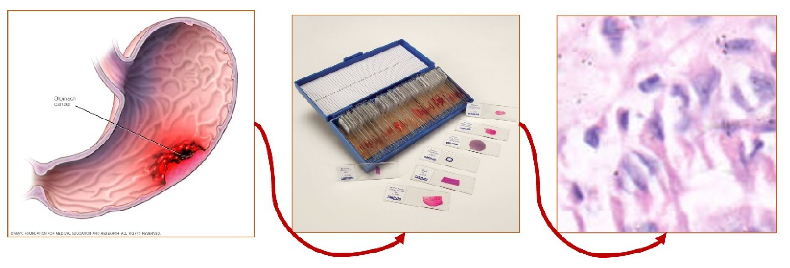
Figure 1. Process of extraction of the Histopathology Image.
Preprints 114097 g001
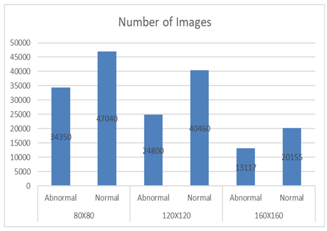
The stomach Histopathology Sub-size Image Database (GasHisSDB) comprises 600 pictures of stomach cancer pathology obtained from a patient's pathological slides from a specific section of the Gastrointestinal tract, each measuring 2048x2048 pixels. The images were obtained by scanning with a NewUsbCamera at a magnification of 20. Four pathologist from Longhua Hospital at the Shanghai University of Traditional Chinese Medicine then provided tissue-specific labeling. In conjunction with five Northeastern University biomedical experts, the photos were cropped into 245,196 sub-sized gastric cancer pathology images. Two qualified pathologist from Liaoning Cancer Hospital and Institute calibrated these pictures. The dataset was then classed as aberrant or normal, with photographs reduced to three different sizes (160x160, 120x120, and 80x80) for each group. The dataset of gastrointestinal images is separated into three sizes: 80x80, 120x120, and 160x160. Each size category is further classified into two groups: Abnormal and Normal. The 80x80 size category has 81,390 photos, with 34,350 classed as Abnormal and 47,040 labeled as Normal. Moving on to the 120x120 size category, there are 65,260 photos altogether, with 24,800 rated as Abnormal and 40,460 as Normal. Finally, in the 160x160 size group, there are 33,272 photos, with 13,117 classified as Abnormal and 20155 as Normal.
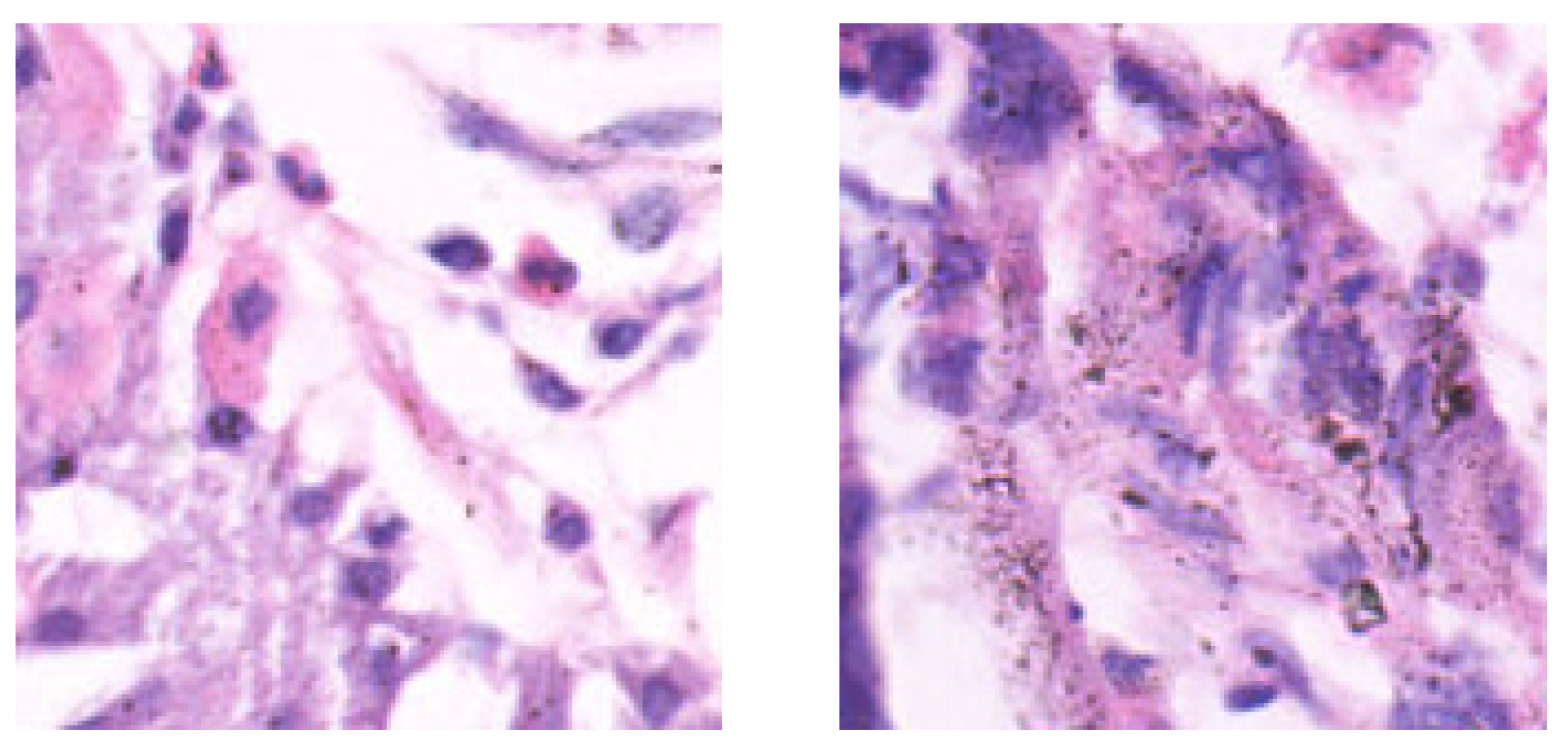
Figure 2. Examples of histopathological Gastric images. (a) Normal tissue and (b) Abnormal tissue.
Preprints 114097 g002
Table 1. Summarises the total number of images for every subclass in an experiment setup.
Preprints 114097 i001
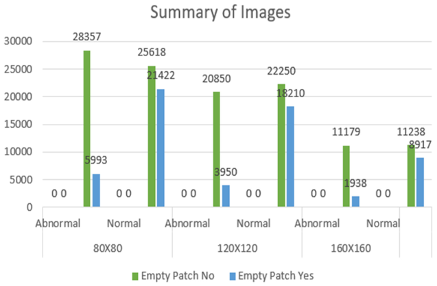
Table 2. Summarises the total number of the Empty and Non-Empty Patch Images in the Dataset.
Preprints 114097 i002

2.3. Methodology Overview

In this work, CNN architectures utilizing transfer learning and ensemble approaches were demonstrated to detect gastric cancer patches. The process is divided into four major steps: (1) creating the dataset through eliminating empty patches and augmenting, (2) tailoring pre-trained networks or base models, (3) choosing the most effective base models to form ensemble models, and (4) assessing and presenting the models using different metrics and the class activation map.
To enhance the model performance, data preprocessing was conducted to create a more balanced dataset by removing non-informative empty patches as the presence of these empty patches would bias the training process and therefore jeopardize the model performance. After empty patches removal, data augmentation was employed to increase the dataset size for training.

2.4. Empty Patch Removal Process

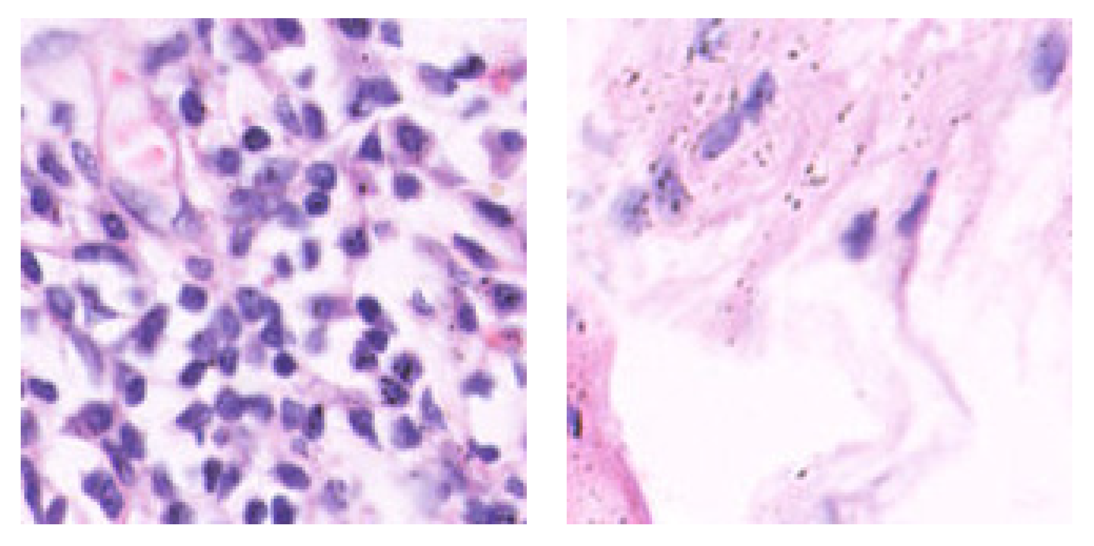
Empty patches are defined as those where more than half of the pixels have an RGB intensity value greater than 230 across all channels. The following is an overview of the empty patch removal procedure, including the proportion of empty patches deleted. In the 120x120 resolution dataset, 15.92% of patches were removed from the abnormal subclass, while 45.01% were removed from the normal subclass. For the 160x160 resolution dataset, 14.77% of patches were removed from the abnormal subclass, and 44.23% were removed from the normal subclass. In the 80x80 resolution dataset, 17.45% of patches were removed from the abnormal subclass, and 45.54% were removed from the normal subclass. After removing these empty patches, the remaining patches were subjected to data training of the model
Figure 3. The pictures above exhibit examples of histopathology: non-empty and empty patch images on the left and right, respectively.
Preprints 114097 g003

2.5. Pretrained networks as Base Models

Convolutional Neural Networks (CNNs) have played an important role in numerous applications since deep learning's inception, due to continual advances in strength, efficiency, and adaptability. CNNs are an excellent illustration of this breakthrough, as they are particularly built for computer vision problems and use convolutional layers inspired by natural visual processes. Multiple CNN structures have evolved throughout time, each improving accuracy, speed, and overall performance, and are usually compared to the ImageNet project, a massive visual database that promotes advancements in computer vision.
Historically, training CNNs from scratch required significant computer resources and time. Transfer learning (TL) provides a practical shortcut by exploiting prior information from trained models to accelerate optimization and perhaps improve classification accuracy. TL entails transferring weights from pre-trained models, using insights acquired from varied datasets, and speeding training processes to improve model accuracy, particularly in complicated architectures [11,12].
ResNet34
Architecture:
ResNet34 is a member of the Residual Networks (ResNet) family, which was introduced by He et al. in 2015. ResNet34 use residual learning to address the issue of vanishing gradients, which is common in deep neural networks. This design is made up of 34 layers, with shortcut connections that allow gradients to flow straight across the network. These residual connections enable the training of very deep networks by overcoming the degradation issue. ResNet34 strikes a balance between depth and computational efficiency, beating shallower networks while maintaining manageable computational costs.
ResNet34 is a variation of ResNet, a CNN architecture created by Microsoft Research. ResNet34 includes 34 layers and uses residual connections to overcome the vanishing gradient problem, making training more efficient. ResNet models are popular due to their efficacy in a variety of applications.
Figure 4. ResNet34 Model Architecture.
Preprints 114097 g004
ResNet50
Architecture:
ResNet50 is a 50-layer version of the ResNet architecture, deeper than ResNet34. This enhanced depth can improve performance on certain tasks, but it also necessitates more computational resources for training.
Figure 5. ResNet50 Model Architecture.
Preprints 114097 g005
VGGNet16
Architecture:
The Visual Geometry Group (VGG) at the University of Oxford developed VGGNet16, a deep CNN architecture. It is well-known for being both simple and successful in picture classification applications. VGGNet16 is made up of 16 layers, the first 13 of which are convolutional, followed by three fully connected layers. Each convolutional layer has a 3x3 kernel, and max-pooling layers are used after a sequence of convolutional layers to minimize spatial dimensions. Although VGGNet16 has a huge number of parameters, which makes it computationally costly, it achieves good accuracy on benchmark datasets thanks to its deep architecture and consistent layer design.
VGGNet, created by the Visual Geometry Group at the University of Oxford, is renowned for its simplicity. It is mostly composed of layered convolutional layers with 3x3 kernels and max-pooling layers. VGGNet includes several variations, including VGG16 and VGG19, which differ in the number of layers.
Figure 6. VGGNet16 Model Architecture.
Preprints 114097 g006
  • Efficientnet Architecture:
EfficientNet is a class of CNN models developed by Google AI that outperforms earlier models using fewer parameters and FLOPs. They employ a novel scaling technique to improve network depth, breadth, and resolution for improved resource management.
Figure 7. EfficientNet Model Architecture.
Preprints 114097 g007
  • VitNet Architecture:
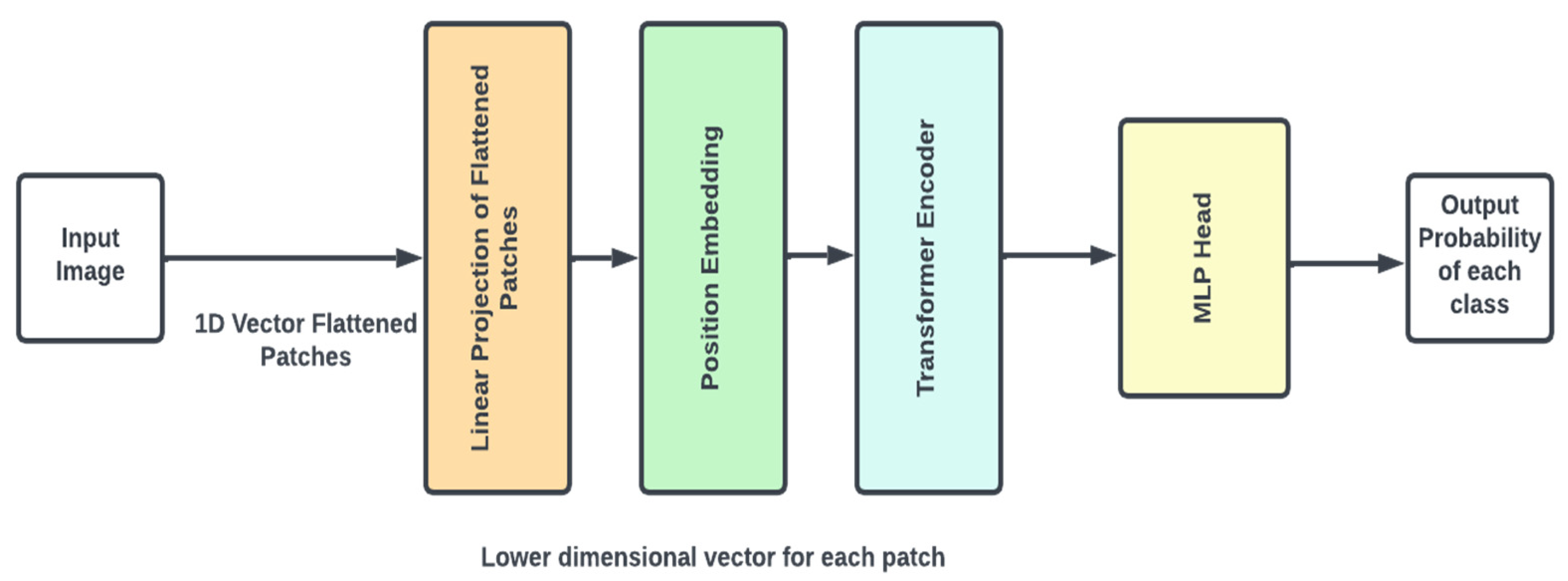
The Vision Transformer is a novel CNN architecture created by Google Research that employs self-attention techniques seen in transformer topologies. Rather than employing convolutional layers like typical CNNs, ViT employs a transformer encoder, which allows it to recognize relationships across large distances in pictures. This method has shown outstanding results in several computer vision tasks, particularly when trained on large datasets.
Figure 8. VITNet Model Architecture.
Preprints 114097 g008
  • Ensemble Architecture:
Convolutional neural networks (CNNs) and transfer learning have significantly increased neural network performance, but there is still potential for improvement. This article proposes the use of ensemble methods to improve the effectiveness of the three models that have been pre-trained. Ensemble learning, a machine learning and statistics-based approach combines the skills of many algorithms to extract relevant insights from data[10].
During this analysis, stacking was determined to be the most appropriate method. This requires training various ML algorithms on the info before merging them to create a composite algorithm capable of successfully combining their input.
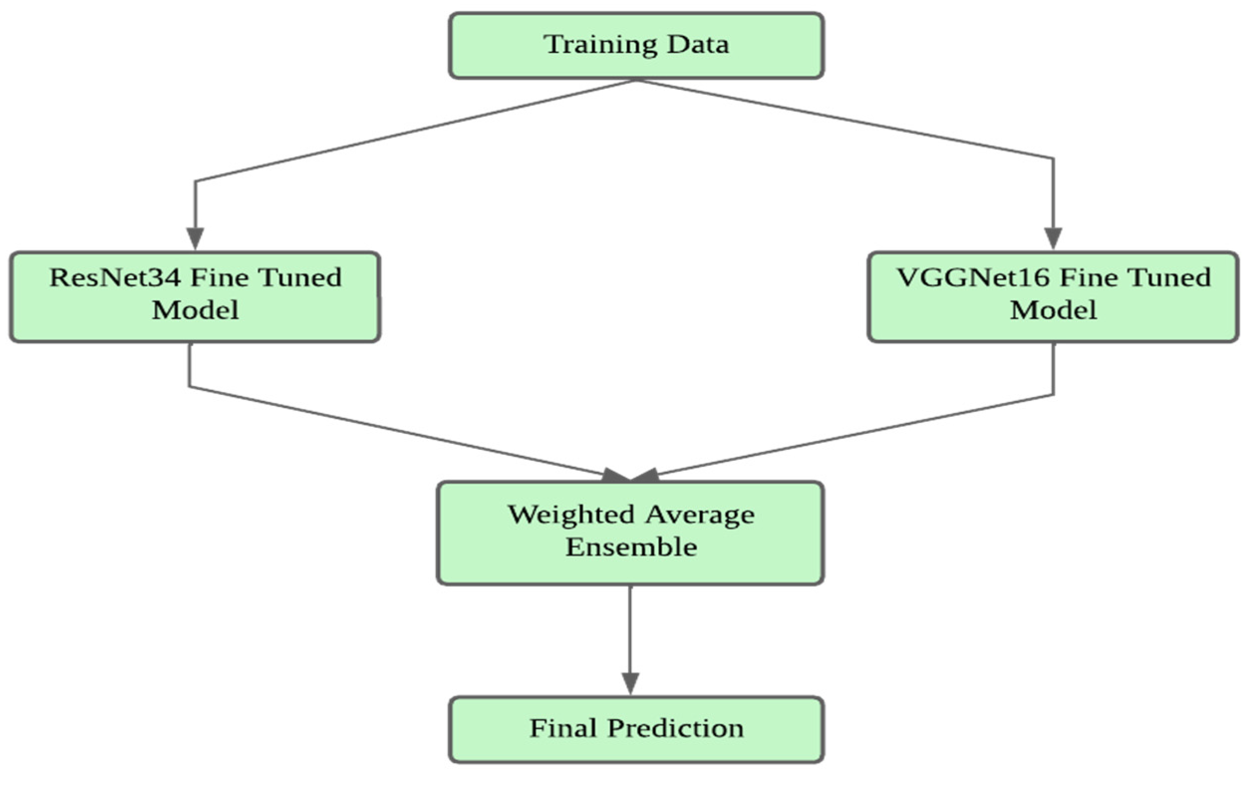
Figure 9. Ensemble Model Architecture.
Preprints 114097 g009
In this research, ensemble model architecture was used using ResNet34 and VGGNet16 as basis models. Initially, each model was trained independently to determine its unique performance. Then selected the best-performing epochs for each model based on validation accuracy. The best-performing epochs were then used to build the ensemble model.
To improve the robustness and generalizability of the ensemble techniques, cross-validation is used. During each fold of the cross-validation approach, the research utilized the best weights from the previous folds to train the ensemble. For example, if cross-validation was done on fold 1, the best epochs from folds 2, 3, 4, and 5 of ResNet34 and VGGNet16 were used to establish the ensemble model.
The ensemble model architecture was created to leverage on the complementary characteristics of ResNet34 and VGGNet16. ResNet34, with its residual connections, successfully mitigates the vanishing gradient problem, allowing for deeper network training. In contrast, VGGNet16, noted for its simplicity and constant layer architecture, excels in capturing fine-grained characteristics. By integrating both models, the ensemble takes use of VGGNet16's comprehensive feature extraction and ResNet34's depth-wise learning capabilities.
Training the ensemble model entailed freezing the early layers of both base models to preserve their pre-trained feature extraction capabilities while fine-tuning the subsequent layers to fit to the unique dataset. This hybrid strategy enabled the ensemble model to outperform individual models, as indicated by improved accuracy and resilience across many validation criteria.In summary, the proposed ensemble model, which included ResNet34 and VGGNet16, showed considerable performance increases. The strategic use of cross-validation and the incorporation of complementary model architectures demonstrate the effectiveness of ensemble techniques in deep learning applications.

2.6. Experimental Setting

The data was divided into training and validation sets. Each network was trained for 20 epochs using 5-fold cross-validation to create the model. The weights from the epoch with the best validation accuracy were chosen as the final representations for each model. Various metrics were then employed to assess accuracy, followed by many objective assessment factors to determine overall performance.

3. Results

The performance evaluation criteria used include accuracy, sensitivity, specificity, Jaccard index, and area under the curve (AUC). Positive samples are those that include abnormal or malignant patches, whereas negative samples contain normal or healthy patches. The phrases true positive (TP), false positive (FP), true negative (TN), and false negative (FN) are used to describe the various prediction results.
1. Accuracy: Accuracy is the ratio of properly identified samples to the total number of samples. It's computed as:
Accuracy = ( T P + T N ) ( T P + T N + F P + F N )
2. Sensitivity (Recall): Sensitivity, also known as recall, is the proportion of real positive samples that the model properly identifies. It’s provided by:
Sensitivity = ( T P ) ( T P + F N )
3. Specificity refers to the fraction of real negative samples properly detected by the model. It's computed as:
Specificity = ( T N ) ( T N + F P )
4. The Jaccard index, commonly known as the Intersection over Union (IoU), assesses the similarity between expected and observed positive samples. It's provided by:
Jaccard   index , = ( T P ) ( T P + F P + F N )
5. Area Under the Curve (AUC): The area under the receiver operating characteristic (ROC) curve, or AUC, relates the true positive rate (sensitivity) to the false positive rate (1 - specificity). A higher AUC implies improved model performance.
By examining these measures, a thorough picture of the model's performance can be acquired, particularly in discriminating between aberrant (positive) and normal (negative) data.
When analyzing the success of machine learning models, performance measures must be considered. These metrics provide numerical numbers that indicate the overall performance of a statistical or machine-learning technique. In classification tasks, performance measures evaluate the model's capacity to accurately categorize data points as well as its consistency in producing the right classifications. Classification accuracy and F1-score are both measures of classification task accuracy, whereas AUC reflects the model's overall ability to forecast accurately. The study's findings, which were obtained by examining these performance metrics, are shown in the table below.
Table 3. The effectiveness of the several deep learning models was assessed using an 80-pixel sub-database, displayed above. The most stunning results are shown in bold.
Model Fold Train Accuracy Train Loss Val Accuracy Val Loss Jaccard Index AUC Specificity Sensitivity
Resnet34 1 98.7508 0.0331 93.6131 0.2175 0.7447 0.9719 0.9604 0.8494
2 97.8192 0.0604 93.7206 0.2092 0.7472 0.9717 0.9638 0.8427
3 98.8546 0.0329 93.8111 0.2210 0.7384 0.9760 0.9699 0.8204
4 97.7773 0.0596 93.8226 0.1724 0.7466 0.9777 0.9625 0.8491
5 98.1767 0.0487 93.7910 0.2399 0.7640 0.9754 0.9518 0.8900
ResNet50 1 98.4818 0.0409 93.7408 0.1936 0.8763 0.8979 0.9682 0.8277
2 96.2419 0.0958 94.2439 0.1880 0.8860 0.9069 0.9703 0.8435
3 98.4410 0.0413 93.4971 0.2024 0.8742 0.9042 0.9577 0.8508
4 97.0654 0.0769 92.7688 0.2016 0.8601 0.9071 0.9431 0.8711
5 93.5411 0.1673 93.8459 0.1869 0.8772 0.9064 0.9648 0.8480
VitNet 1 83.6243 0.3631 83.7591 0.3555 0.6945 0.7132 0.9347 0.4916
2 82.9835 0.3816 84.2836 0.3490 0.6969 0.7076 0.9493 0.4660
3 78.4974 0.4755 78.8656 0.4560 0.5946 0.5054 0.9988 0.0121
4 82.5612 0.3898 84.2841 0.3505 0.6986 0.7015 0.9488 0.4542
5 78.3217 0.5231 77.4105 0.5353 0.5674 0.5 1 0
VggNet 1 98.7371 0.0366 93.7591 0.2579 0.8763 0.9746 0.9747 0.8053
2 96.2693 0.0969 94.3341 0.1785 0.8868 0.9757 0.9738 0.8353
3 98.5683 0.0417 93.9220 0.2120 0.8763 0.9751 0.9720 0.8178
4 94.3224 0.1519 93.7681 0.1621 0.8756 0.9733 0.9685 0.8245
5 98.3636 0.0487 93.7910 0.2329 0.8768 0.9724 0.9693 0.8302
EfficientNet 1 74.9474 0.5035 75.4057 0.5142 0.6094 0.7478 0.7172 0.7784
2 82.4435 0.3866 83.0474 0.3685 0.6829 0.6726 0.9421 0.4030
3 81.0359 0.4139 82.3709 0.3855 0.6704 0.6346 0.9463 0.3229
4 82.3379 0.3879 84.2231 0.3531 0.6975 0.6725 0.9419 0.4030
5 82.6571 0.3805 83.5210 0.3651 0.6944 0.6816 0.9401 0.4232
Ensemble 1 98.3587 0.0436 99.3430 0.0252 0.9867 0.9904 0.9957 0.9850
2 98.5187 0.0410 99.2421 0.0211 0.9839 0.9875 0.9962 0.9787
3 98.6001 0.0384 99.2056 0.0237 0.9836 0.9898 0.9936 0.9861
4 97.9234 0.0627 97.8197 0.0651 0.9562 0.9642 0.9886 0.9398
5 98.5642 0.0390 99.0869 0.0221 0.9823 0.9866 0.9943 0.9789
Table 4. The effectiveness of the several deep learning models was assessed using a 120-pixel sub-database, displayed above. The most stunning results are shown in bold.
Model Fold Train Accuracy Train Loss Val Accuracy Val Loss Jaccard Index AUC Specificity Sensitivity
Resnet34 1 98.8627 0.0327 96.8167 0.1097 0.8347 0.9879 0.9812 0.9075
2 99.2847 0.0187 97.0297 0.1327 0.8444 0.9815 0.9884 0.8884
3 98.9145 0.0336 96.9364 0.1025 0.8392 0.9907 0.9901 0.8762
4 99.1640 0.0234 96.4475 0.1208 0.8175 0.9879 0.9836 0.8778
5 99.2957 0.0214 96.6893 0.1074 0.8149 0.9897 0.9877 0.8642
ResNet50 1 99.5552 0.0125 96.7257 0.1120 0.9316 0.9518 0.9756 0.9281
2 99.2449 0.0213 96.9856 0.1156 0.9372 0.9254 0.9951 0.8557
3 99.7229 0.0089 97.0930 0.1198 0.9388 0.9493 0.9833 0.9154
4 99.5007 0.0142 96.8166 0.1253 0.9339 0.9379 0.9853 0.8905
5 99.5042 0.0147 97.0748 0.0995 0.9379 0.9406 0.9860 0.8951
VitNet 1 86.6963 0.3109 87.4715 0.2875 0.7518 0.7395 0.9488 0.5301
2 84.6948 0.3495 86.1826 0.3185 0.7254 0.7123 0.9470 0.4775
3 82.2817 0.4486 81.7531 0.4287 0.6310 0.5 1 0
4 85.7447 0.3298 87.9123 0.2929 0.7581 0.7607 0.9464 0.5750
5 84.2084 0.3465 86.3265 0.3085 0.7231 0.6767 0.9582 0.3951
VggNet 1 76.6185 0.4764 75.6162 0.5053 0.6152 0.7657 0.7776 0.7538
2 88.3740 0.2758 89.1768 0.2611 0.7889 0.7476 0.9592 0.5361
3 88.1351 0.2822 88.3388 0.2732 0.7756 0.7372 0.9605 0.5139
4 86.6576 0.3140 88.2826 0.2813 0.7673 0.6979 0.9591 0.4368
5 88.3702 0.2745 88.4198 0.2781 0.7779 0.7460 0.9594 0.5325
EfficientNet 1 99.1949 0.0265 96.8167 0.1372 0.9340 0.9878 0.9867 0.8818
2 99.8978 0.0054 96.9416 0.1716 0.9363 0.9886 0.9873 0.8884
3 98.4339 0.0464 97.1824 0.1130 0.9403 0.9883 0.9901 0.8897
4 96.4544 0.1011 96.0322 0.1098 0.9176 0.9860 0.9757 0.8905
5 99.8366 0.0061 96.9614 0.1410 0.9338 0.9902 0.98363 0.9005
Ensemble 1 97.2581 0.0728 97.6125 0.0646 0.9501 0.9593 0.9853 0.9332
2 97.7973 0.0622 98.1738 0.0533 0.9627 0.9647 0.9913 0.9381
3 97.7894 0.0603 97.8756 0.0618 0.9531 0.9636 0.9874 0.9399
4 97.8457 0.0625 97.5778 0.0685 0.9486 0.9549 0.9876 0.9223
5 98.9735 0.0316 99.4250 0.0226 0.9872 0.9895 0.9965 0.9826
Table 5. The effectiveness of the several deep learning models was assessed using a 160-pixel sub-database, displayed above. The most stunning results are shown in bold.
Model Fold Train Accuracy Train Loss Val Accuracy Val Loss Jaccard Index AUC Specificity Sensitivity
Resnet34 1 99.6311 0.0132 97.9807 0.0648 0.8949 0.9961 0.9887 0.9398
2 99.5496 0.0148 98.1776 0.0656 0.9022 0.9913 0.9922 0.9341
3 99.7337 0.0083 98.1038 0.0535 0.8928 0.9976 0.9912 0.9308
4 97.1184 0.0896 97.2005 0.0821 0.8665 0.9931 0.9806 0.9361
5 99.5437 0.0213 98.4187 0.0738 0.9105 0.9929 0.9862 0.9739
ResNet50 1 99.3660 0.0288 98.4396 0.0579 0.9678 0.9739 0.9904 0.9573
2 99.5842 0.0170 98.3143 0.0592 0.9628 0.9719 0.9894 0.9544
3 99.8263 0.0066 98.1038 0.0776 0.9599 0.9684 0.9874 0.9494
4 99.9538 0.0018 97.9348 0.0743 0.9574 0.9620 0.9903 0.9338
5 99.7718 0.0112 98.3708 0.0625 0.9648 0.9832 0.9839 0.9826
VitNet 1 82.2614 0.4526 81.6888 0.4532 0.6295 0.5 1 0
2 84.4919 0.3426 86.2870 0.3141 0.7307 0.6980 0.9555 0.4405
3 81.9212 0.4638 83.0248 0.4527 0.6543 0.5 1 0
4 84.3706 0.3502 84.6718 0.3393 0.6977 0.6841 0.9498 0.4184
5 82.0483 0.3951 86.3919 0.3069 0.7274 0.6337 0.9776 0.2898
VggNet 1 77.3246 0.4784 76.5826 0.4820 0.6291 0.7732 0.7643 0.7822
2 90.0875 0.2296 93.0702 0.1838 0.8607 0.7924 0.9604 0.6244
3 91.0623 0.2155 92.8018 0.1911 0.8572 0.8139 0.9641 0.6636
4 91.0069 0.2178 93.0925 0.1655 0.8589 0.8168 0.9628 0.6709
5 91.4476 0.2077 92.0146 0.1945 0.8444 0.8186 0.9659 0.6712
EfficientNet 1 99.9769 0.0014 98.2101 0.1121 0.9623 0.9946 0.9915 0.9398
2 99.6882 0.0098 97.9498 0.0795 0.9584 0.9944 0.9952 0.9088
3 98.8773 0.0347 97.9683 0.0896 0.9579 0.9921 0.9934 0.9122
4 99.2738 0.0244 97.2005 0.0940 0.9464 0.9912 0.9834 0.9243
5 99.6692 0.0091 98.1312 0.0814 0.9586 0.9948 0.9896 0.9391
Ensemble 1 98.4785 0.0412 98.8067 0.0313 0.9751 0.9829 0.9910 0.9749
2 99.0877 0.0268 98.9066 0.0325 0.9753 0.9775 0.9955 0.9594
3 99.1203 0.0298 99.1873 0.0260 0.9830 0.9866 0.9945 0.9787
4 99.4813 0.0150 99.7246 0.0079 0.9942 0.9964 0.9977 0.9952
5 98.9165 0.0319 99.3291 0.0245 0.9836 0.9901 0.9948 0.9855

4. Discussion

In this work, the proposed model was trained on datasets with varied picture sizes, such as 80x80 and 120x120 and 160X160. Findings highlights the critical significance of ongoing innovation and exploration in increasing medical machine learning and hence improving healthcare practices. Notably, the findings shows that the top five ensemble models had high detection accuracy across all sub-databases. The overall ensemble model demonstrated the highest accuracy, surpassing the performance of VGGNet, ResNet34, and ResNet50, which also outperformed VitNet and EfficientNet. The only exception was in the 160 × 160 sub-database, where EfficientNet achieved an accuracy of 92%. By combining multidisciplinary techniques and technology breakthroughs, can pave the way towards a future in which early and precise identification of gastrointestinal disorders is not only achievable but also common practice in protecting human health and well-being.
This deliberate method was used to assist the model build a solid knowledge of multiple picture dimensions, making it more flexible to a variety of real-world scenarios. Nonetheless, it is worth noting that proposed model's knowledge may have been expanded much more with greater computing resources. Greater computational capability might have enabled a more in-depth examination of the dataset's intricacies, as well as the discovery of insights beyond existing capabilities.
These advanced methodologies offer various structures and improvement tactics that may increase the efficacy of the model. Time restrictions precluded the incorporation of these algorithms into the current system; nonetheless, their use holds great promise for improving cancer detection techniques.
This research prioritizes in innovation and placing people at the heart of the research. The objective is to make research applications as user-friendly as possible while also emphasizing how they might benefit medical practitioners. This research strive to integrate the most recent research work with practical applications, avoiding plagiarism and crafting a research story that is honest and true to research’s commitment to expanding scientific understanding.

4.1. Future Directions

In the future, focus will be on two major goals: developing an easy-to-use web app for cancer detection and expanding current algorithms to include new forms of cancer. The primary goal of this research is to develop a model that will work for all forms of cancer, not just specific ones. This will be accomplished by utilizing many data sources and innovative algorithms to obtain a thorough understanding of cancer, hence assisting healthcare professionals with diagnosis.By integrating multidisciplinary methodologies and capitalizing on technological developments, probably will work towards that in future in which early and precise identification of GI problems is not only possible, but also the standard for protecting human health and well-being.

5. Conclusion

Detecting and diagnosing gastrointestinal (GI) illnesses is critical for human health, yet it can be challenging owing to limited medical competence and expensive expenses. Using machine learning, particularly deep learning techniques, has the potential to increase the speed and accuracy of GI illness identification. This research study investigated the efficiency of ensemble approaches using five pre-trained models on the Gastric Histopathology Sub-size Image Database (GasHisSDB), which comprises a diverse set of pictures in various pixel sizes and categories. Considerable boost in prediction accuracy can be seen when utilizing ensemble learning, which combines the predictive skills of several models, as opposed to using individual models and previous studies that used comparable datasets. This demonstrates the potential of ensemble approaches to improve the capabilities of medical machine learning systems, resulting in more effective and precise diagnoses.
Current approach is based on transfer learning, a technique that improves model learning by leveraging knowledge from previously trained models. Moreover employed an ensemble strategy to improve performance by merging various classifiers. Following a rigorous review, current approach revealed a great accuracy on the test dataset, exceeding current evaluation techniques. This demonstrates how deep learning may help alleviate the pressure on healthcare systems while also improving human health outcomes. [21,22]
In this study, advanced deep ensemble learning models were created that used transfer learning from multiple pre-trained networks, including VitNet, EfficientNet, VGGNet, ResNet34, and ResNet50, to improve stomach cancer diagnosis. The study found that using base models in ensemble learning resulted in high identification accuracy (97.57% to 99.72%) for histopathology pictures with resolutions ranging from 80 × 80 pixels to 160 × 160 pixels.
The experimental results demonstrated that ensemble models may extract key information even from smaller picture patches while retaining good performance. This improvement implies the possibility of adopting digital scanners with lower specifications, as well as reduced data storage and computing needs for histopathology operations. This, in turn, might speed up stomach cancer identification and perhaps increase survival rates. Continued work in these areas is intended to push the boundaries of medical image processing and enhance clinical results.However, it is critical to recognize the limits of the current research. The usage of a restricted dataset emphasizes the need to have access to larger, higher-quality datasets to enhance and confirm the approaches. Furthermore, computational restrictions may have influenced the scope of the results. Future studies might look at introducing new preprocessing methods and optimizing algorithms to boost performance. Furthermore, the field of medical image retrieval offers several chances for continuous research, including the ability to use multiple deep-learning approaches and models for complete examination.

Supplementary Materials

The following supporting information can be downloaded at the website of this paper posted on Preprints.org. The GasHisSDB dataset is openly available at this Link: https://paperswithcode.com/dataset/gashissdb.

Funding

This research received no funding.

Institutional Review Board Statement

Not applicable.

Informed Consent Statement

Informed consent was obtained from all subjects involved in the study.

Data Availability Statement

Not applicable.

Acknowledgments

We would like to express our deepest gratitude to the Roux Institute, the IEAI and the Alfond Foundation for their invaluable support and contributions.

Conflicts of Interest

The authors declare no conflict of interest.

References

  1. Rai, H.M. Cancer detection and segmentation using machine learning and deep learning techniques: a review. Multimedia Tools Appl. 2023, 83, 27001–27035. [Google Scholar] [CrossRef]
  2. Kuntz, S.; Krieghoff-Henning, E.; Kather, J.N.; Jutzi, T.; Höhn, J.; Kiehl, L.; Hekler, A.; Alwers, E.; von Kalle, C.; Fröhling, S.; et al. Gastrointestinal cancer classification and prognostication from histology using deep learning: Systematic review. Eur. J. Cancer 2021, 155, 200–215. [Google Scholar] [CrossRef] [PubMed]
  3. Mirza, O.M.; Alsobhi, A.; Hasanin, T.; Ishak, M.K.; Karim, F.K.; Mostafa, S.M. Computer Aided Diagnosis for Gastrointestinal Cancer Classification Using Hybrid Rice Optimization With Deep Learning. IEEE Access 2023, 11, 76321–76329. [Google Scholar] [CrossRef]
  4. Suzuki, H.; Yoshitaka, T.; Yoshio, T.; Tada, T. Artificial intelligence for cancer detection of the upper gastrointestinal tract. Dig. Endosc. 2021, 33, 254–262. [Google Scholar] [CrossRef] [PubMed]
  5. Yasmin, F.; Hassan, M.; Hasan, M.; Zaman, S.; Bairagi, A.K.; El-Shafai, W.; Fouad, H.; Chun, Y.C. GastroNet: Gastrointestinal Polyp and Abnormal Feature Detection and Classification With Deep Learning Approach. IEEE Access 2023, 11, 97605–97624. [Google Scholar] [CrossRef]
  6. Yong, M.P.; Hum, Y.C.; Lai, K.W.; Lee, Y.L.; Goh, C.-H.; Yap, W.-S.; Tee, Y.K. Histopathological Gastric Cancer Detection on GasHisSDB Dataset Using Deep Ensemble Learning. Diagnostics 2023, 13, 1793. [Google Scholar] [CrossRef] [PubMed]
  7. Sivari, E.; Bostanci, E.; Guzel, M.S.; Acici, K.; Asuroglu, T.; Ayyildiz, T.E. A New Approach for Gastrointestinal Tract Findings Detection and Classification: Deep Learning-Based Hybrid Stacking Ensemble Models. Diagnostics 2023, 13, 720. [Google Scholar] [CrossRef] [PubMed]
  8. Gunasekaran, H.; Ramalakshmi, K.; Swaminathan, D.K.; J, A.; Mazzara, M. GIT-Net: An Ensemble Deep Learning-Based GI Tract Classification of Endoscopic Images. Bioengineering 2023, 10, 809. [Google Scholar] [CrossRef] [PubMed]
  9. Su, Q.; Wang, F.; Chen, D.; Chen, G.; Li, C.; Wei, L. Deep convolutional neural networks with ensemble learning and transfer learning for automated detection of gastrointestinal diseases. Comput. Biol. Med. 2022, 150, 106054. [Google Scholar] [CrossRef] [PubMed]
  10. R. A. Almanifi, M. A. M. Razman, I. M. Khairuddin, M. A. Abdullah and A. P. P. A. Majeed, "Automated Gastrointestinal Tract Classification Via Deep Learning and The Ensemble Method," 2021 21st International Conference on Control, Automation and Systems (ICCAS), Jeju, Korea, Republic of, 2021, pp. 602-606, doi: 10.23919/ICCAS52745.2021.9649754. keywords: {Deep learning;Automation;Stacking;Predictive models;Control systems;Gastrointestinal tract;Data models;Gastrointestinal tract;Colorectal cancer;Deep learning;CNN;Transfer learning;Ensemble}. [CrossRef]
  11. Haile, M.B.; Salau, A.; Enyew, B.; Belay, A.J. Detection and classification of gastrointestinal disease using convolutional neural network and SVM. Cogent Eng. 2022. [Google Scholar] [CrossRef]
  12. Billah, M.; Waheed, S. Gastrointestinal polyp detection in endoscopic images using an improved feature extraction method. Biomed. Eng. Lett. 2017, 8, 69–75. [Google Scholar] [CrossRef] [PubMed]
  13. Chao, W.-L.; Manickavasagan, H.; Krishna, S.G. Application of Artificial Intelligence in the Detection and Differentiation of Colon Polyps: A Technical Review for Physicians. Diagnostics 2019, 9, 99. [Google Scholar] [CrossRef]
  14. Li, B.; Meng, M.Q.-H. Automatic polyp detection for wireless capsule endoscopy images. Expert Syst. Appl. 2012, 39, 10952–10958. [Google Scholar] [CrossRef]
  15. Guo, L.; Gong, H.; Wang, Q.; Zhang, Q.; Tong, H.; Li, J.; Lei, X.; Xiao, X.; Li, C.; Jiang, J.; et al. Detection of multiple lesions of gastrointestinal tract for endoscopy using artificial intelligence model: a pilot study. Surg. Endosc. 2020, 35, 6532–6538. [Google Scholar] [CrossRef] [PubMed]
  16. Charfi, S.; El Ansari, M.; Balasingham, I. Computer-aided diagnosis system for ulcer detection in wireless capsule endoscopy images. IET Image Process. 2019, 13, 1023–1030. [Google Scholar] [CrossRef]
  17. Wang, X.; Qian, H.; Ciaccio, E.J.; Lewis, S.K.; Bhagat, G.; Green, P.H.; Xu, S.; Huang, L.; Gao, R.; Liu, Y. Celiac disease diagnosis from videocapsule endoscopy images with residual learning and deep feature extraction. Comput. Methods Programs Biomed. 2019, 187, 105236. [Google Scholar] [CrossRef] [PubMed]
  18. Renna, F.; Martins, M.; Neto, A.; Cunha, A.; Libânio, D.; Dinis-Ribeiro, M.; Coimbra, M. Artificial Intelligence for Upper Gastrointestinal Endoscopy: A Roadmap from Technology Development to Clinical Practice. Diagnostics 2022, 12, 1278. [Google Scholar] [CrossRef]
  19. Liedlgruber, M.; Uhl, A. Computer-Aided Decision Support Systems for Endoscopy in the Gastrointestinal Tract: A Review. IEEE Rev. Biomed. Eng. 2011, 4, 73–88. [Google Scholar] [CrossRef] [PubMed]
  20. Naz, J.; Sharif, M.; Yasmin, M.; Raza, M.; Khan, M.A. Detection and Classification of Gastrointestinal Diseases using Machine Learning. Curr. Med Imaging Former. Curr. Med Imaging Rev. 2021, 17, 479–490. [Google Scholar] [CrossRef] [PubMed]
  21. Ghanzouri, I.; Amal, S.; Ho, V.; Safarnejad, L.; Cabot, J.; Brown-Johnson, C.G.; Leeper, N.; Asch, S.; Shah, N.H.; Ross, E.G. Performance and usability testing of an automated tool for detection of peripheral artery disease using electronic health records. Sci. Rep. 2022, 12, 1–11. [Google Scholar] [CrossRef]
  22. Singh, A.; Wan, M.; Harrison, L.; Breggia, A.; Christman, R.; Winslow, R.L.; Amal, S. Visualizing Decisions and Analytics of Artificial Intelligence Based Cancer Diagnosis and Grading of Specimen Digitized Biopsy: Case Study for Prostate Cancer. In Proceedings of the Companion Proceedings of the 28th International Conference on Intelligent User Interfaces; Association for Computing Machinery: New York, NY, USA, March 27, 2023; pp. 166–170. [Google Scholar]
Disclaimer/Publisher’s Note: The statements, opinions and data contained in all publications are solely those of the individual author(s) and contributor(s) and not of MDPI and/or the editor(s). MDPI and/or the editor(s) disclaim responsibility for any injury to people or property resulting from any ideas, methods, instructions or products referred to in the content.
Copyright: This open access article is published under a Creative Commons CC BY 4.0 license, which permit the free download, distribution, and reuse, provided that the author and preprint are cited in any reuse.
Prerpints.org logo

Preprints.org is a free preprint server supported by MDPI in Basel, Switzerland.

Subscribe

© 2024 MDPI (Basel, Switzerland) unless otherwise stated