1. Introduction
Artificial Intelligence (AI) dates back to 1950 as described in [
1], where computers were used to simulate intelligent behavior. John McCarthy described this act of simulating intelligence as AI. What began as a simple software program, AI is now advanced includes several complex algorithms, and can even perform functions similar to a human brain. AI has evolved significantly over the last few years, especially with Machine Learning (ML) and Deep Learning (DL) advent. According to [
2] ML is an evolving branch of computational algorithms designed to emulate human intelligence. ML algorithms can learn from past data and improve their predictive accuracy over time. ML has paved its way into the healthcare industry, making its applications seamless. Its applications include diagnosing diseases and predicting the therapeutic response as mentioned in [
1]. Several literatures have also stated that it is possible to detect early stages of cancer [
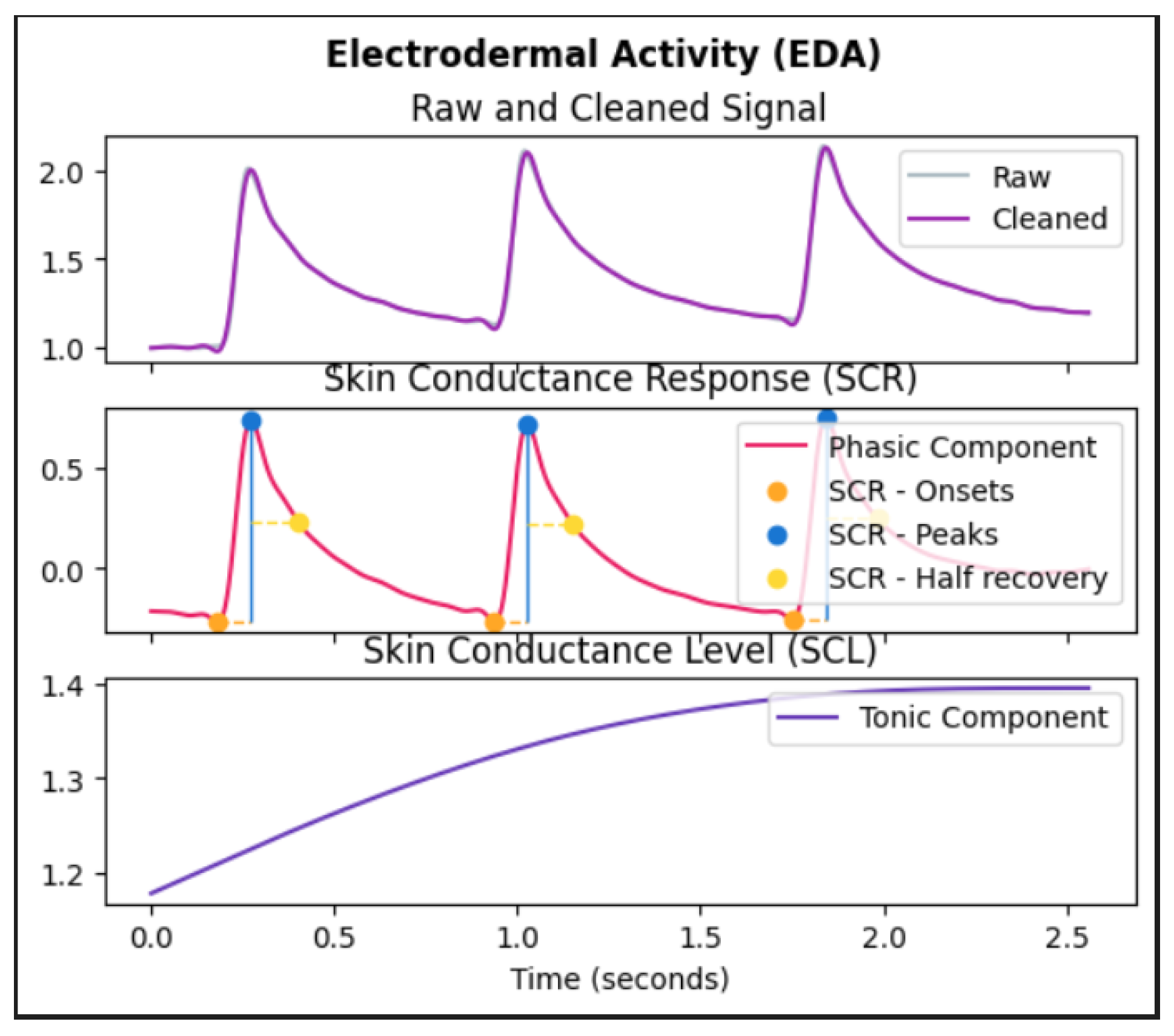
3] which was almost impossible in the past. Although AI was already studied in the mid-90s, its applications in medicine were limited because of the problem of "overfitting" and this limitation was overcome in the 2000s with the availability of larger datasets and several regularization methods. Because of ML’s ability to analyze large datasets and identify minor patterns that are not possible through conventional techniques, it can be used to identify pain in humans. Pain is a complex phenomenon, and according to [
4] pain is defined as "an unpleasant sensory and emotional experience". Despite knowledge and technology, pain is still often poorly managed [
5,
6], and this mostly affects patients with limited communication abilities, who cannot report their pain experience. Such vulnerable groups are infants and elderly people making it difficult for medical professionals to come to a concrete conclusion or solution. ML techniques driven by data hold significant potential in automating pain recognition, thereby assisting healthcare professionals in delivering appropriate medical interventions and treatments. This automatic pain recognition could be done in several ways such as through facial expressions, speech, body movements, and/or by using biophysical signals such as Electromyography (EMG), Electrocardiogram (ECG), Electrodermal activity (EDA/GSR). Numerous challenges such as memorization, sensitivity to adversarial examples, and overfitting hinder the effectiveness of machine learning models. Several techniques are aimed to overcome these obstacles. One such approach is the mixup [
7] that has been proven to enhance the performance. Despite its success, the mixup has yet to be applied to physiological signals. Motivated by this methodology, this literature aims to incorporate the mixup strategy to investigate whether it enhances the performance of pain recognition models.
Either ML or DL could be used for pain recognition, in this literature the conventional ML approach is used wherein relevant features are extracted manually with the help of a feature extractor. This high-level input data representation is subsequently used to optimize an inference model. Such approaches have proven to be effective. Pain recognition can be done using numerous approaches by utilizing physiological signals, some of them by extracting hand-crafted features and then using them to train the ML model, others using a DL architecture. The authors of [
8] have proposed a classification architecture based on Deep Belief Networks (DBNs) to classify pain using photoplethysmography signals. Here the DBNs were trained using a set of manually engineered features, so a permutation and combination of different methodologies are possible. While ML models have enabled significant breakthroughs, they also exhibit undesirable behaviors such as memorization and sensitivity to adversarial samples, reducing the performance and generalization capabilities of these models. One solution to overcome this unexpected behavior is data augmentation. [
9]Data augmentation is the method of choice to train on similar but different examples to the training data. Data augmentation improves the generalization and performance of ML algorithms by applying transformations such as rotations, translations, and flips. However, the procedure is dataset-dependent and thus requires the use of expert knowledge. Data augmentation also assumes that the examples in the vicinity share the same class, and does not model the vicinity relatation across samples of different classes. These issues motivated the authors of [
7] to introduce a simple and data-agnostic data augmentation technique called "mixup". Mixup has gained significant attention and has been shown to enhance the robustness and accuracy of ML and DL models. Mixup involves blending pairs of samples and their corresponding labels to create new synthetic training examples. Mixup takes two samples,
, and
, and their associated labels,
, and
, and creates new examples
and
as weighted linear combinations.
The equations can be represented as below:
where (
,
) and (
,
) are two samples drawn at random from the extracted features as mentioned in [
7]. Here,
is a random value drawn from a beta distribution with a user-defined parameter
, typically set between 0.1 and 0.4. The generated synthetic example
and the label
are used as input during training. While previous works have demonstrated the effectiveness of mixup, they have been limited to images, sound, and text data. As part of this literature, Mixup is applied to physiological signals that are then used to train conventional machine learning algorithms/models to recognize pain. A comparison is drawn between machine learning architectures that integrate mixup and those that do not utilize mixup. It is possible to apply mixup on time-series data because the two samples,
, and
are raw input vectors [
7] not limited to images. At the end of this work, it is proved that mixup could also be done on time-series data like EDA signals, eventually leading to a better performance.
This paper is organized as follows.
Section 2 summarizes the latest techniques available for pain recognition and the current methodology used to perform mixup.
Section 3 explains the proposed method and the datasets and pre-processing in detail. The results are discussed in
Section 4 and the paper is concluded with future recommendations in
Section 5.
2. Literature Review
As stated in the previous sections, it is difficult to interpret pain, especially when the patient cannot communicate his or her pain experience. Detecting pain has always been tricky because there is no easy method to measure and detect the presence of pain directly, most of the methods available in the past relied solely on techniques such as verbal communication and tend to lack reliability. However, advancements in artificial intelligence have eased the process of pain recognition, by offering automated detection of medical symptoms. Artificial intelligence requires a large amount of data with which it learns to be able then to make predictions on unseen data. The authors in [
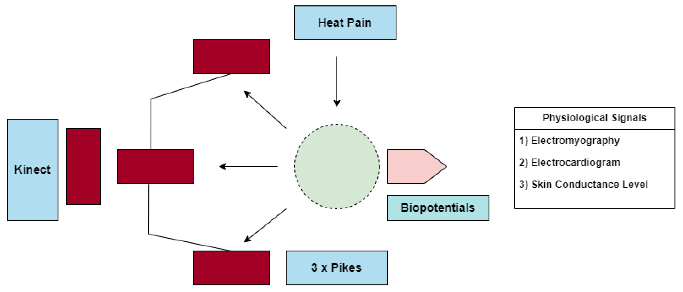
10] present a multimodal data set, in which pain is induced at different levels. The data set is called the Biopotential and Video (BioVid) Heat Pain Database and this dataset is used for research purposes. This section presents some of the well-established machine learning approaches, some of them making use of the BioVid dataset for pain recognition, additionally, mixup a data augmentation technique, and its prior applications in domains like speech and images have been covered.
There is constantly growing work focusing on pain recognition using physiological signals as also stated in [
11]. Categorization is then based on the nature of pain elicitations. Many authors have proposed traditional machine learning approaches such as decision trees or support vector machines (SVM) that involve using a set of carefully engineered features extracted from raw data. The extracted features are then used to optimize an inference model. Some of them are worth noting. In [
12], a pain detection approach based on Electroencephalogram (EEG) signals is proposed. Choi-Williams quadratic time-frequency distribution was used to extract necessary features from EEG signals, and then the extracted features were used to train an SVM which was then able to recognize pain based on the classification task. In [
13] camera Photoplethysmography (PPG) signals were combined with ECG and EMG signals, and the dataset that was then obtained was used for pain intensity classification based on a fusion architecture at the feature level with SVMS and Random Forests as base classifiers. Authors in [
14,
15] have used the BVDB [
16] to perform different pain intensity classification experiments based on a carefully selected set of features extracted from both physiological and video signals, classification task was then performed based on Random Forest and SVM classifiers. In [
17] a user-independent pain intensity classification evaluation based on physiological signals using the same dataset has been done. An adaptive confidence learning approach for personalized pain estimation was also proposed by the same authors based on both physiological and video modalities, the fusion was applied at the feature level. Here Random Forests were used to solve the regression task.
Authors of [
8] have proposed a classification approach based on Deep Belief Networks (DBNs). The work mainly focuses on the assessment of patient’s pain levels during surgery, using photoplethysmography (PPG) signals. However, it is to be noted that in [
8] the proposed architecture has been built on a set of manually engineered features extracted from PPG signals.
Now that we have seen the benefits of machine learning techniques, especially in pain detection, the efficiency of these techniques might be limited because they exhibit undesirable behaviors on adversarial examples and unseen data that impact the overall performance. Several solutions have been proposed to overcome these undesirable behaviors, mixup [
7] a data augmentation technique, is one such solution to overcome these limitations. Mixup [
7] trains a neural network on convex combinations of pairs of examples and their labels. Authors of [
7] have conducted experiments on the ImageNet-2012, CIFAR-10, CIFAR-100, and speech data showing that the mixup improves the generalization of state-of-the-art neural network architectures. It is also found that mixup reduces the memorization of corrupt labels, additionally, mixup also increases the robustness to adversarial examples and along with it stabilizes the training of generative adversarial networks.
While mixup proposed by the authors of [
7] works by linearly interpolating inputs and their corresponding labels, it is shown in [
18] that the samples can also be mixed in a non-linear fashion, the authors of [
18] have named this technique "nonlinear Mixup". Unlike linear mixup where the input and output label pairs share the same, linear, scalar mixing policy, the nonlinear mixup approach embraces nonlinear interpolation policy for both the input and their corresponding labels, the mixing policy for the labels is adaptively learned based on the mixed input. Experiments have been done on benchmark sentence classification datasets and it is indicated that nonlinear mixup plays a vital role in improving the performance of the classification model. The study conducted by [
19] demonstrates the effectiveness of mixup data augmentation in natural language processing (NLP).
Mixup technique is used extensively in the field of health care, especially for medical image classification. In [
20] a technique called Balanced-Mixup has been proposed for highly imbalanced medical image classification. In this approach, a balanced mixup simultaneously performs regular and balanced sampling of the training data. The resulting two sets of samples are then mixed up to create a more balanced training distribution from which a neural network can effectively learn without incurring heavily under-fitting the minority classes. Authors of [
21] examined the effectiveness of mixup in enhancing the performance of a COVID-19 image classification model. They conducted a comparative analysis between traditional methods and those methods that incorporated mixup. Their findings consistently indicated that the models using mixup augmentation surpassed those relying solely on conventional methods, underscoring the superiority of mixup in enhancing classification accuracy.
So far we have seen various methods that have been proposed and put into practice for pain recognition. These methods involve accessing physiological signals and employing machine learning algorithms to automatically detect pain in patients without relying on their verbal communication. We also saw a popular data augmentation technique called mixup and its ability to enhance the efficiency of deep learning architectures on unfamiliar and adversarial examples, however, it is important to note that, the input data to machine learning or deep learning models that are designed for medical applications are not only images, but they can also be other forms of data such as physiological signals as discussed. It is necessary for such models working on raw physiological signals to perform well on test data and adversarial instances failing which the pain recognition model overfits and becomes unreliable for pain recognition. However, though there are many proposals explaining the benefits of mixup most of them focus mainly on images as input data but for time-series input data like EDA, ECG, and EMG the behavior of mixup is unknown.
In our current work, we focus on a novel approach that employs the mixup strategy on features derived from time-series signals like EDA. Subsequently, we utilize the augmented data to train our machine learning model after which the efficiency of the machine learning model is seen to be better than the models without mixup. These findings illustrate a significant enhancement in machine learning models when incorporating mixup, unlike previous methods that do not utilize mixup.
4. Results
Validating a machine learning model is an important aspect as it not only helps us understand the model better but also estimates an unbiased generalization performance, it plays an important role in identifying and correcting overfitting enabling us to select the best model for a given task. There is no single validation method that works in all scenarios. This section discusses a few validation techniques comparing the pain recognition models employed with and without Mixup.
4.1. Leave One Subject Out Cross Validation (LOSOCV)
Cross-validation is a technique used to train and test machine learning models. In cross-validation, the machine learning model is trained on a subset of data points and tested with the remaining data and this is repeated in a loop for n times, n being the number of cross folds. A common approach when multiple subjects are involved is to use leave-one-subject cross-validation (LOSOCV). LOSOCV involves iterating through each subject in a dataset of n subjects. During each iteration, one subject is left out as a test set while the model is trained on the remaining n-1 subjects. This process is repeated until all the subjects have been used as test sets exactly once. When a subject is dropped out, all observations from the subject are left out of the training set. In our work, the value of n is 87, since we have 87 subjects involved in the experiment.
The pain recognition model with mixup performed better in this experimental setup than the model without mixup. The mixup was performed using equations (
1) and (
2) as mentioned in [
7]. where (
,
) and (
,
) are two samples drawn at random from the extracted features and
. The
values are sampled from the Beta distribution.
The Beta distribution is utilized because it effectively models random variables that are constrained within a specific range, typically between 0 and 1, making it suitable for representing probabilities. Its shape parameter, alpha, often shows a pronounced peak near the extremes of 0 or 1. This indicates a high likelihood of observing values close to these limits, suggesting a strong tendency toward extreme outcomes, where the data sample is categorized as one class. Meanwhile, the distribution maintains variability within the range, with a somewhat constant probability of selecting values in the middle (0.33 as likely as 0.5 for instance). This implies that while extreme outcomes are more probable, values closer to the center are still feasible. The parameter leads to improved performance, smaller creates less mixup effect, whereas, for larger mixup leads to underfitting.
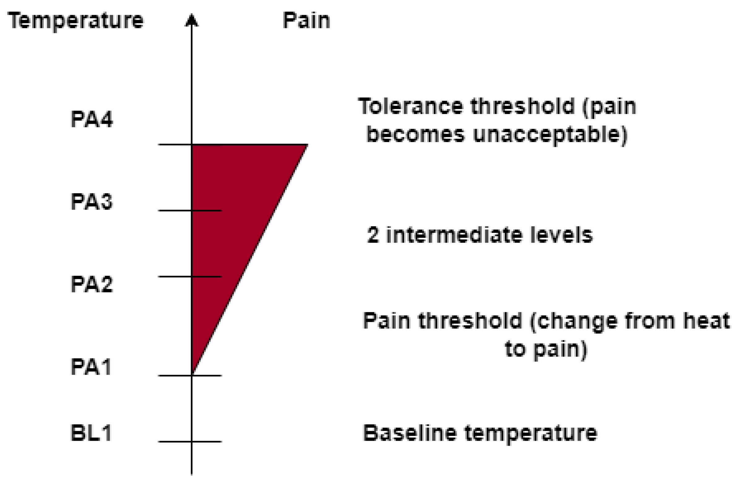
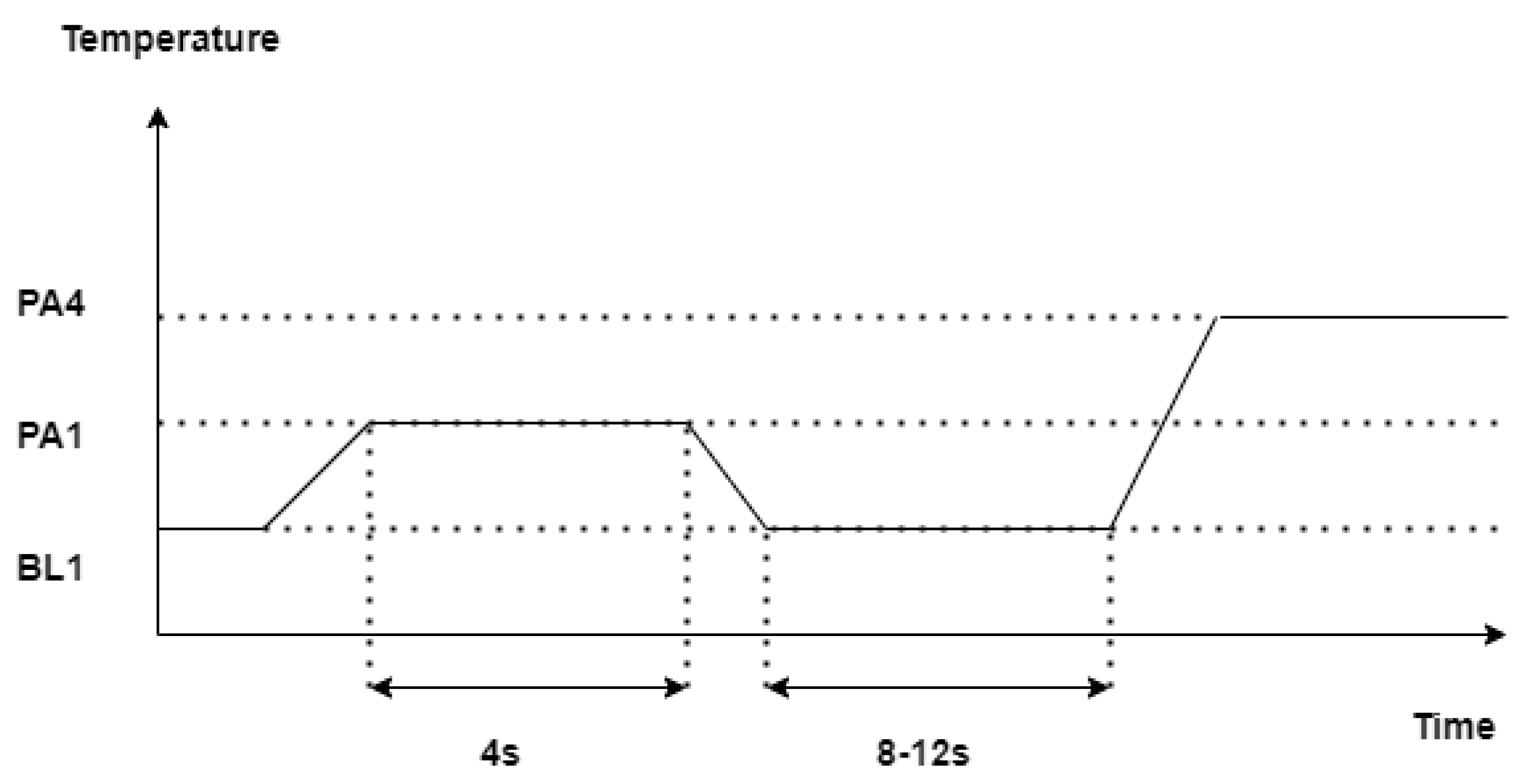
A performance evaluation based on the average accuracy of the designed architectures in a binary classification task consisting of the discrimination between the baseline temperature BL1 and the pain tolerance temperature PA4 is reported in
Table 1.
At a glance, the designed models with Mixup performed better than the models without Mixup. The average accuracy of the classical machine learning model trained as a binary classifier was 74.61 % without mixup data augmentation. However, when the data was augmented with mixup the performance turned out to be better, is the hyperparameter that can be tuned, where [0,1]. Further, is sampled from the Beta distribution, the classifier was trained with different values of and the performance of the classical machine learning model was the best when = 0.1 where the average accuracy of the pain recognition model showed up to be 75.87%.
4.2. Wilcoxon Signed Rank Test
Wilcoxon signed-rank test is a non-parametric hypothesis test that compares the median of two paired groups and tells if they are identically distributed or not. Wilcoxon signed-rank test is also known as the Wilcoxon matched pair test. It can be used when the differences between the pairs of data are non-normally distributed. This test is used for comparing two machine learning models. The working of a Wilcoxon test can be briefly explained in a few steps:
The null (h0) and alternate (h1) hypothesis are determined. Null Hypothesis (ho): The median difference between the paired samples is zero, or there is no difference between the two related populations. Alternate Hypothesis (h1): The median difference between the paired samples is not zero, indicating a difference between the two related populations.
A difference (D) is calculated between each pair of observations.
The pairs with zero differences are discarded.
We find out the absolute differences and assign ranks to them starting from the lowest to the highest.
The Sum of ranks for positive and negative differences are calculated separately.
The smaller sum of ranks(W) is used as the test statistic.
Obtained value W is compared with the critical value from the Wilcoxon signed-rank distribution table or the p-value is calculated.
The obtained p-value is compared with a so-called significance level which is typically set to 0.05, the null hypothesis is rejected if the p-value is less than the significance level and we can conclude that there is a statistically significant difference between the two models/ populations. On the contrary, if the obtained p-value is greater than the significance level, it is an indication that there is no statistically significant difference between the populations/models. In our experiment, the p-values were less than 0.05 for all values of indicating that the ML models incorporating mixup performed better than the ones without mixup.
As part of our experiment, we compared the machine learning models with and without mixup by using the Wilcoxon-signed-rank test, and the p-value is calculated for two lists of accuracy scores: one obtained by performing a LOSOCV on a machine learning model without mixup and the other obtained by performing a LOSOCV on a machine learning model with mixup. The p-value obtained was compared with a significance value and it was much smaller than 0.05 indicating statistical significance which means that the null hypothesis could be rejected hence proving that the machine learning model with mixup performed better than the model without mixup.
4.3. Confusion Matrix
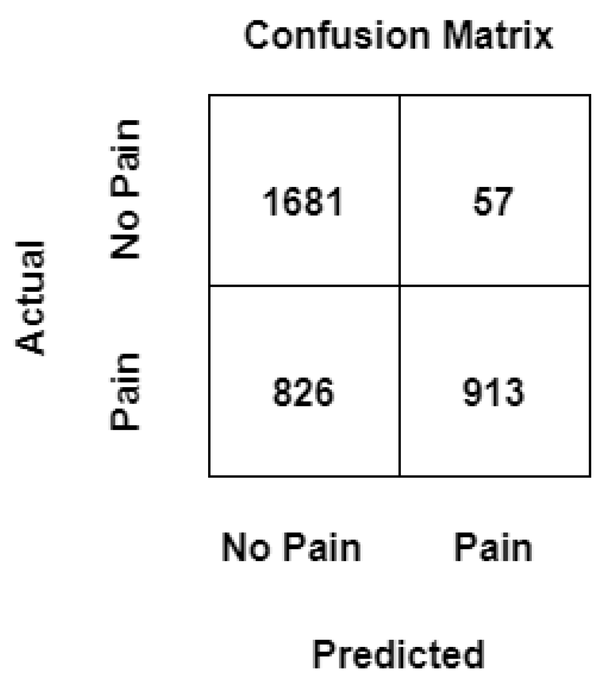
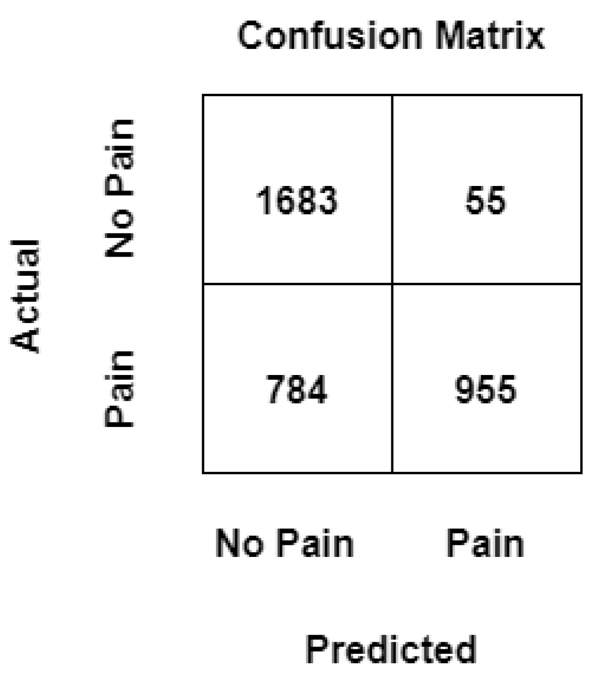
In machine learning, to measure the performance of a model, a confusion matrix is used where exact allocation is possible as it displays the accurate and inaccurate instances based on the model’s predictions. The matrix displays the number of instances produced by the model on the test data. A comparison is made within the realm of pain recognition, assessing a conventional machine learning model trained on manually extracted statistical features, with and without the utilization of mixup, and the results are summarized in
Figure 6 and
Figure 7 respectively.
True Positive (TP): Number of events correctly predicted as "pain" by the ML model.
True Negative (TN): Number of events correctly predicted as "no pain" by the ML model.
False Positive (FP): It is the total count of events predicted as "pain" by the ML model when the actual value is "no pain".
False Negative (FN): It is the total count of events predicted as "no pain" by the model when the actual value is "pain".
It can be noticed that values that have been previously wrongly predicted as "no pain" by the machine learning model without mixup are corrected by the machine learning model with a mixup with a hyperparameter value set to 0.1, and the model can classify these events as "pain" correctly, likewise, two instances that have been wrongly classified as "pain" by the machine learning model without mixup has been correctly classified as "no pain" when the same model is trained with augmented data. It can be observed that the architectures can consistently discriminate between the baseline temperature BL1 and pain tolerance temperature PA4, the architectures that use augmented data through Mixup perform better than their counterparts without Mixup.
4.4. ROC Curve
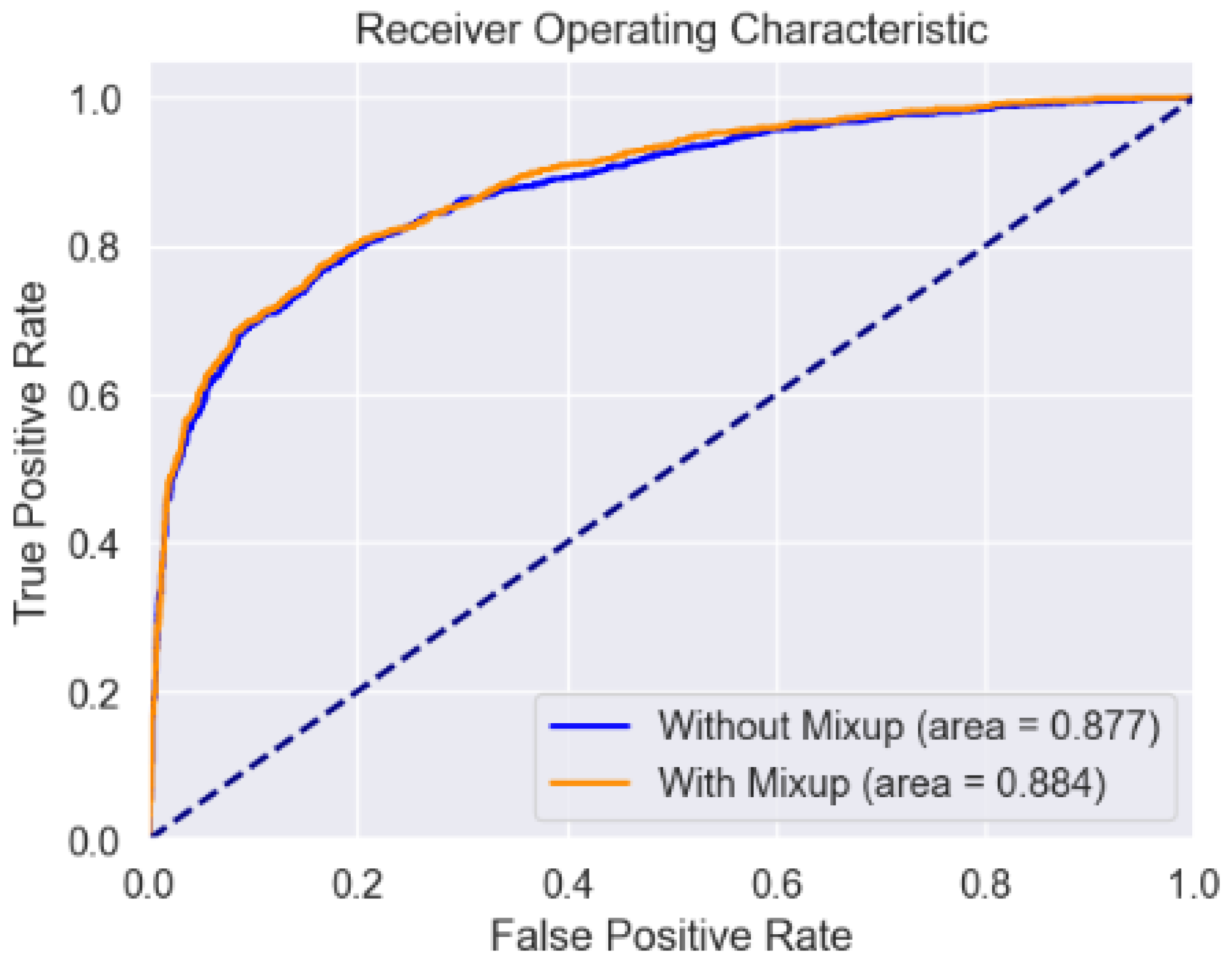
A ROC curve or receiver operating characteristic curve has also been illustrated which is nothing but a graphical plot demonstrating the performance of a binary classifier at varying threshold values.
In our study, we evaluated the performance of an ML model with and without mixup using a receiver operating characteristic (ROC) curve. It was observed that the ROC curve for the ML model trained without mixup resulted in an Area Under the Curve (AUC) of 0.877. When the model was trained with mixup we obtained an AUC of 0.884 suggesting an improvement in the model’s performance compared to the model that was trained without mixup. This increase demonstrates the effectiveness of the mixup in enhancing the model’s performance which has been designed to recognize pain in humans.
5. Conclusions and Future Work
This section includes a summary of the research conducted and its future scope. This literature explored the application of mixup, a data-agnostic and straightforward data augmentation principle for pain intensity classification based on physiological data focusing on EDA. We explored machine-learning architectures that could effectively be used for this application with and without mixup. We used the BioVid Heat Pain Database (PART A) and designed a binary classifier to be able to distinguish between BL1("no pain") and PA4("pain"). An SVM was used for this purpose that was trained with and without augmented data. The data augmentation that was used is called mixup. Incorporating mixup into the training pipeline required only a few lines of code and introduced minimal computational overhead. comparison between architectures employing mixup and those that were trained without augmented data was made and it was observed that the performance of the models using mixup was better than the ones without mixup. All designed architectures were trained comprehensively, within the constraints of the computational resources available for model development. Therefore, refining different components of the models through additional adjustments is believed to enhance the system’s performance potentially. The efficacy of mixup augmentation relies heavily on the parameter , which determines the extent of augmentation and thus requires a careful investigation to achieve a better performance. Several other additional experiments were also conducted such as nonlinear mixup and Nonlinear mixup proved to have a higher potential for further research.
Mixup also opened up several possibilities for further exploration. First, as part of this work, the primary focus of this study was not on achieving the highest accuracy for the pain recognition model. Rather, the aim was to validate the concept of mixup by applying it to a time-series EDA signal. Basic machine learning architectures were employed for this purpose, which may result in lower accuracy compared to other works of literature utilizing more advanced architectures. There is a potential to explore the suggested mixup approach further by implementing it on a neural network-based architecture, in [
22] the authors have used a random forest classifier instead of a support vector machine to achieve an accuracy of 73.80% by using only EDA signals and an average accuracy of 74.10% using an early fusion technique. In literature [
17] the average accuracy of the machine learning model with more features extracted is reported to be 81.10% using only EDA signals and 82.73% by using all three signals ECG, EDA, and EMG. It is possible to apply mixup on the architectures proposed in other literature to observe the impact on the overall performance of the model. Another approach worth exploring for the EDA signals is the application of nonlinear mixup, as proposed in [
18]. Further, the application of linear interpolation was showcased using two randomly selected samples, additionally, it would also be possible to explore mixing varying numbers of samples for future investigation. Lastly, the possibility of applying the mixup technique to other learning problems such as unsupervised learning can also be explored.
