1. Introduction
Currently, physicians use low-dose CT scans to detect nodules and tumors [
1], but Stage 1 non-small-cell tumors can be between 0.5 - 3cm, making detection a challenging task. Even when this task is performed by a specialist, the error rate is 27-47% [
2,
3]. When a nodule is detected, a specialist will make a classification according to standard descriptions, relying heavily on their own experience, leading to high levels of variance. This lack of consistency can be addressed by Machine Learning algorithms. But with the black box nature of machine learning, algorithms are unable to explain the output they produce which affects trust and credibility in the results. A common solution to this is segmentation models as they produce heat maps. A related concern is how to effectively process 3D image data generated by most medical scans. Models which directly process 3D data have high computational requirements and therefore need to be simpler [
4]. For this reason, large pre-trained 3D segmentation models are not common and sophisticated 2D models are much more robust at segmentation and classification tasks. The common concern when converting 3D data to 2D is the loss of spatial positioning. This research addresses that concern, testing if that loss can be compensated by other benefits. In addition, current machine learning techniques often disregard the clinical process which utilizes information such as patient information, visual information, and biomarkers [
5]. These are important factors and need to be a part of AI models. But these types of models have been avoided due to both the inaccessibility of multimodal data in the past and the complex model architectures required to build an accurate model.
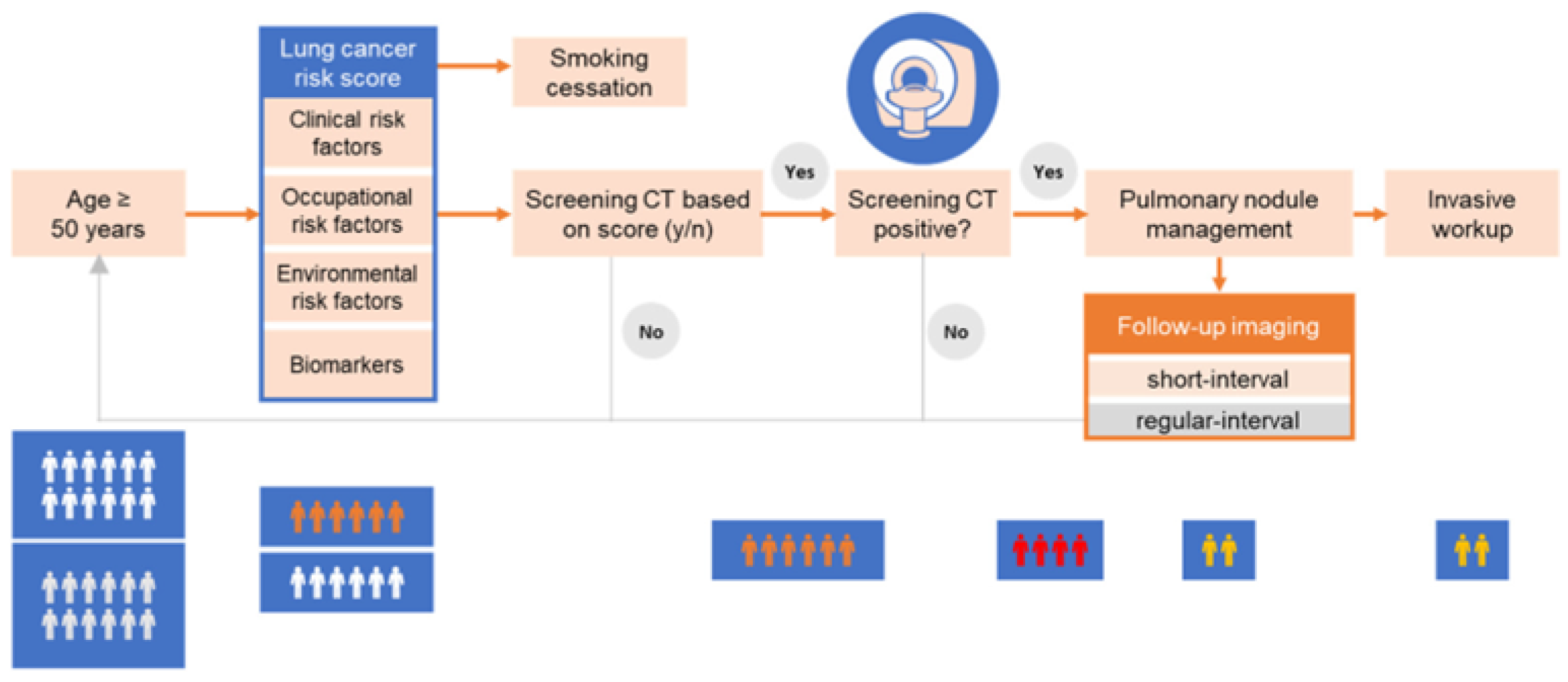
Figure 1.
Clinical Workflow.
Figure 1.
Clinical Workflow.
As annotated datasets have become available publicly, multiple models have been produced for the task of lung cancer classification and segmentation. S. Primakov et al. produced a 3D segmentation model which was trained on 1328 total samples and achieved a DICE score of 0.82, sensitivity of 0.97 and specificity of 0.99 [
6]. This is the state-of-the-art 3D segmentation model currently and is a good baseline to serve as a comparison for the imaging section of my model. Next, S. Zhang et al. hold the state-of-the-art lung tumor classification model through the fine-tuning of LeNet-5 (a 2D model), achieving an accuracy of 97.04 [
7]. The findings from these papers all support the value of the proposed method.
In addition to annotated datasets, multimodal datasets have been produced for the task of lung nodule and cancer detection. The primary dataset available is LUCAS, created by Daza et al. who also created a baseline model for others to build upon [
8]. The model utilized a custom version of AlignedXception fitted for 3D for classification, which was then combined with a basic MLP. This model achieved ROC, AP, and F1 scores of 0.71, 0.09, and 0.25 respectively, highlighting the difficulty of working with multiple modalities. Roa et al. worked with Daza et al. to create a more advanced model called SAMA [
9]. The aggregation layer uses a dynamic filter which generates a dynamic response map which gets concatenated, weighted and turned into a probability. This model was able to achieve an AP and F1 score of 0.251 and 0.341. The third attempt to utilize the LUCAS dataset was made by Barrett et al. who created a custom 3D CNN for classification based on AlignedXception and an encoder decoder system for the biomarkers [
10]. This final approach achieved an F1, ROC, and AP of 0.508, 0.847, and 0.53 making this the state-of-the-art model.
In this paper, I propose a model that fine-tunes the DeepLabv3-resnet-101 architecture with data from MSDL composed of 64 low dose CT scans [
11]. This model is then combined with a larger model that processes the biomarkers and aggregates both outputs through fully connected layers to achieve a final confidence score. The full multimodal model was trained on the LUCAS dataset containing 830 low dose CT scans with corresponding patient information files. To measure the accuracy of the model, AP, ROC, and F1 scores were used as they allow for the best comparison to past models and build consistency. For the segmentation model, DICE coefficient was the main metric used but recall and specificity were also measured.
2. Materials and Methods
2.1. Tools
All coding for this project was done in Python 3.7, using PyTorch to implement the models. Other important packages were nibabel, med2image, and numpy all used for the conversion, loading, and editing of the CT scans. Models were built, trained and tested using Google Collaboratory (Colab).
2.2. Data
2.2.1. MSD
The MSD Task06_Lung was used for the training of the segmentation model. The dataset consisted of ninety-six thin-section (<1.5mm) positive samples from different patients with a corresponding annotated file that outlined the tumor. The patients had non-small-cell lung cancer and the mask file was marked by an expert radiologist. Out of the ninety-six files, thirty-two were marked for testing and had no corresponding mask file (dataset was originally used for a competition), leaving sixty-four to train on.
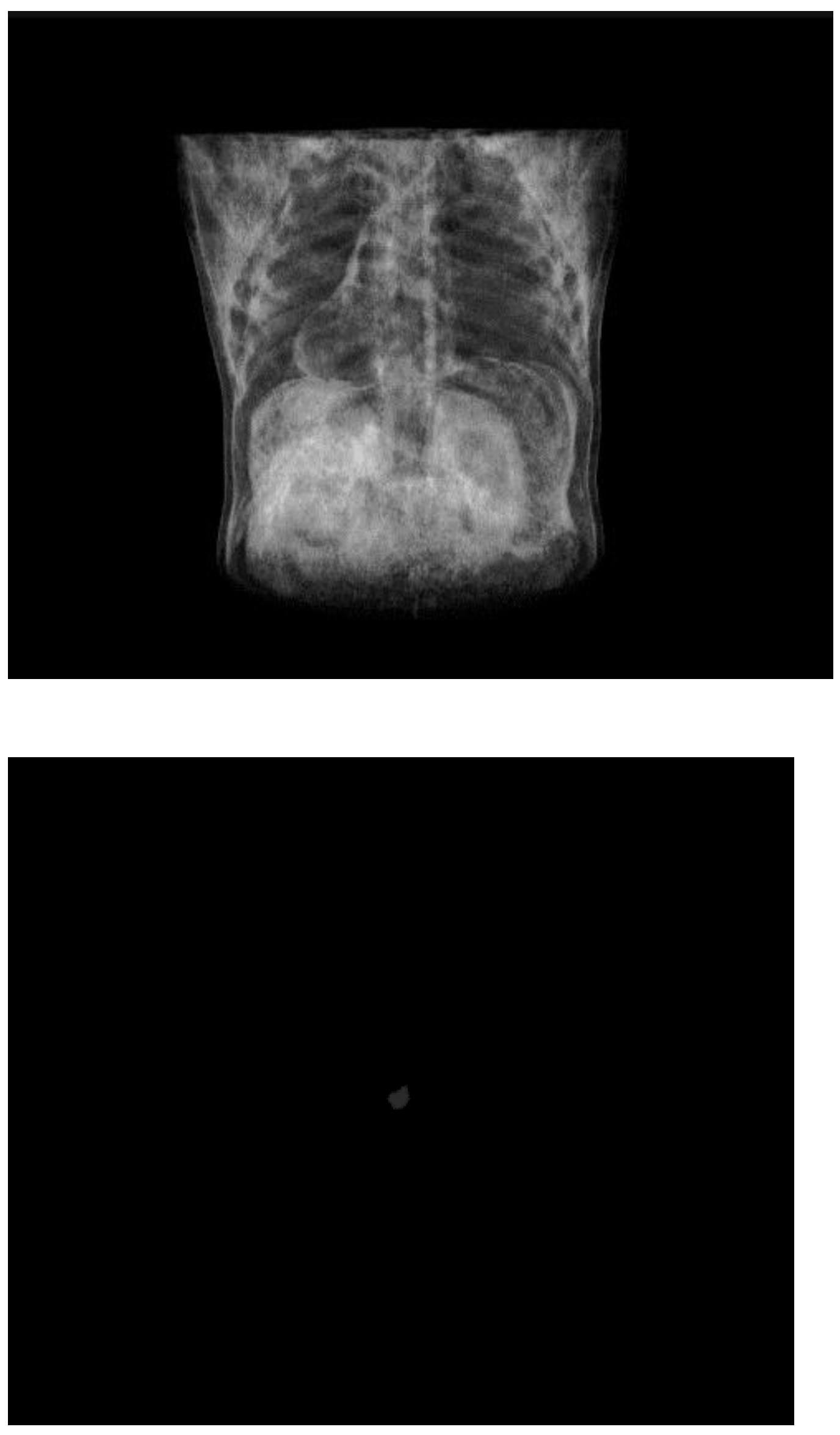
Figure 2.
View of original 3D CT scan with its corresponding mask from MSD dataset.
Figure 2.
View of original 3D CT scan with its corresponding mask from MSD dataset.
2.2.2. LUCAS
There were a total of 830 scans with 72 of them being positive (8.5%). The scans were taken in a clinical setting and were diagnosed by an expert physician. Many of the patients had respiratory diseases or had a high risk of developing lung cancer. Of the 830 scans, 20% (166) were set aside for testing. Due to the heavy imbalance in data, the choice was made to balance the dataset and use an equal amount of positive and negative files, leading to 104 training files. The biomarkers contained 77 different values which covered patient information, visual information, and internal markers.
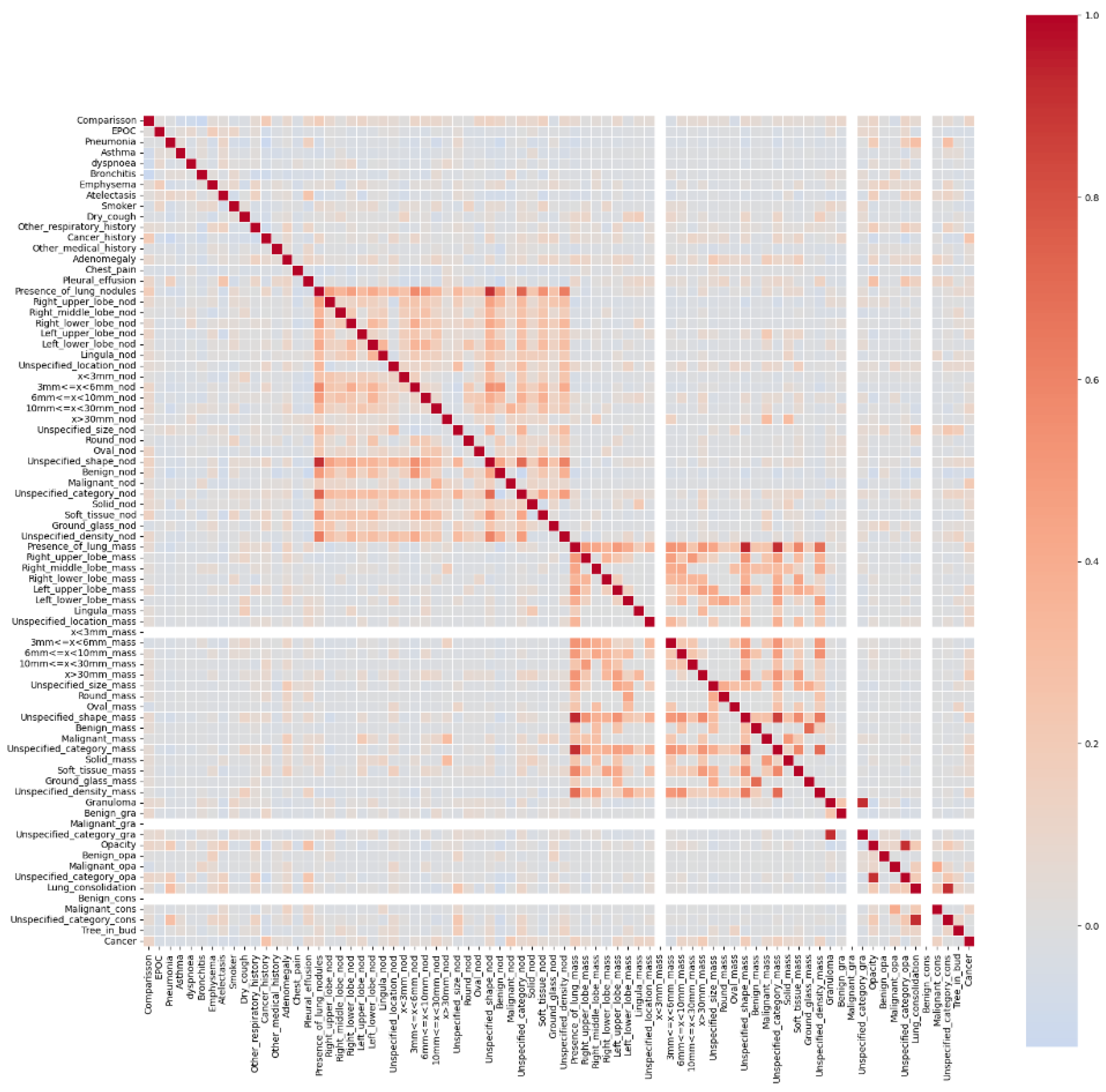
Figure 3.
Correlation of biomarkers with Cancer.
Figure 3.
Correlation of biomarkers with Cancer.
2.3. Preprocessing
2.3.1. MSDL
Each Nifti (NII) file was split along the z-axis into 300-700 slices at 512x512 resolution using the med2image library. Conversion of all scans resulted in 17,000 slices, 90% of which did not contain a visible tumor in the corresponing mask. Data was filtered to only keep those with the tumor, resulting in 1756 files. The original dataset (In 3D) was 13 gigabytes, and the new dataset was 356 megabytes (36.5x smaller).
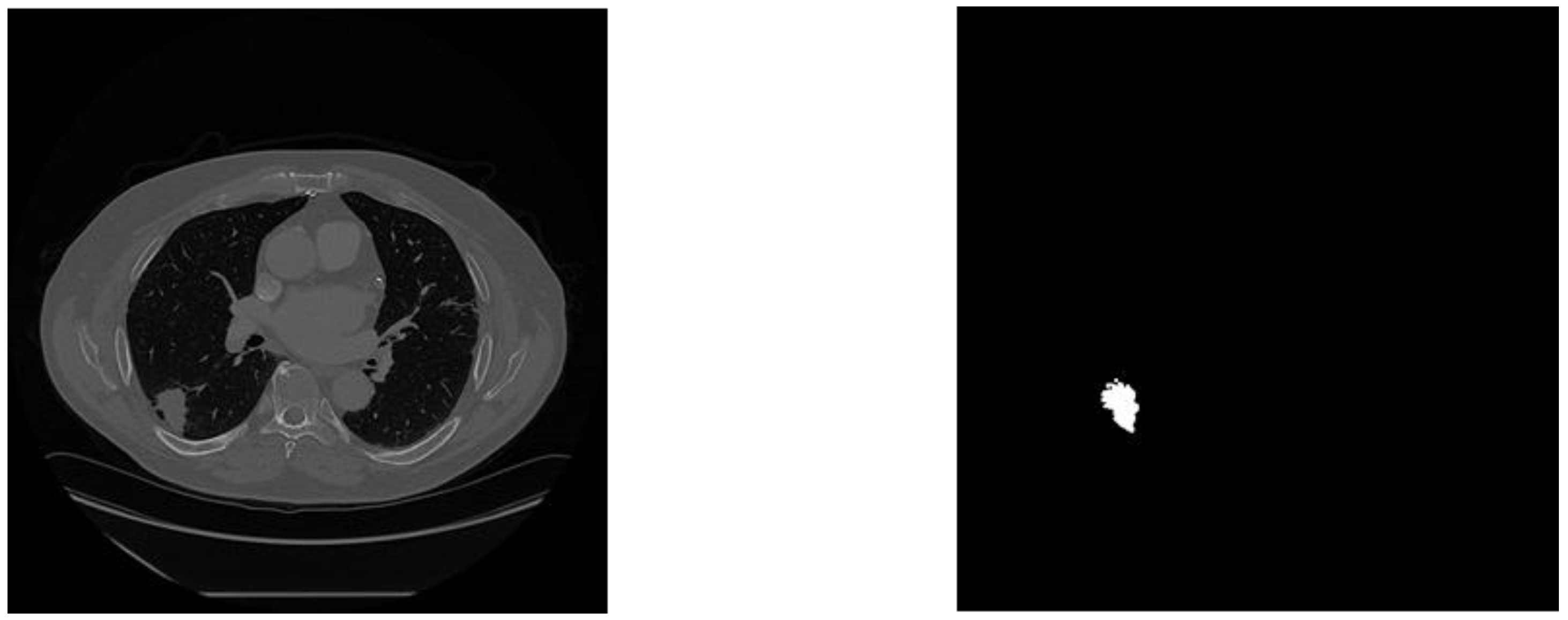
Figure 4.
Example training image with its corresponding mask.
Figure 4.
Example training image with its corresponding mask.
2.3.2. LUCAS
All images were resized to 256x256x256 (height, width, slices) to reduce compute processing needs and create consistency. A Z-score normalization was applied to all slices to ensure internal consistency of each image. Finally, if any images were below the necessary size, they were symmetrically padded.
2.4. Model Architecture
2.4.1. Segmentation Model
The segmentation model architecture used was DeepLabv3-ResNet-101. This specific architecture was used as it is one of the best performing models on the Pascal-Voc test [
12]. It has also proven effective in working with lung CT scans as shown by Polat [
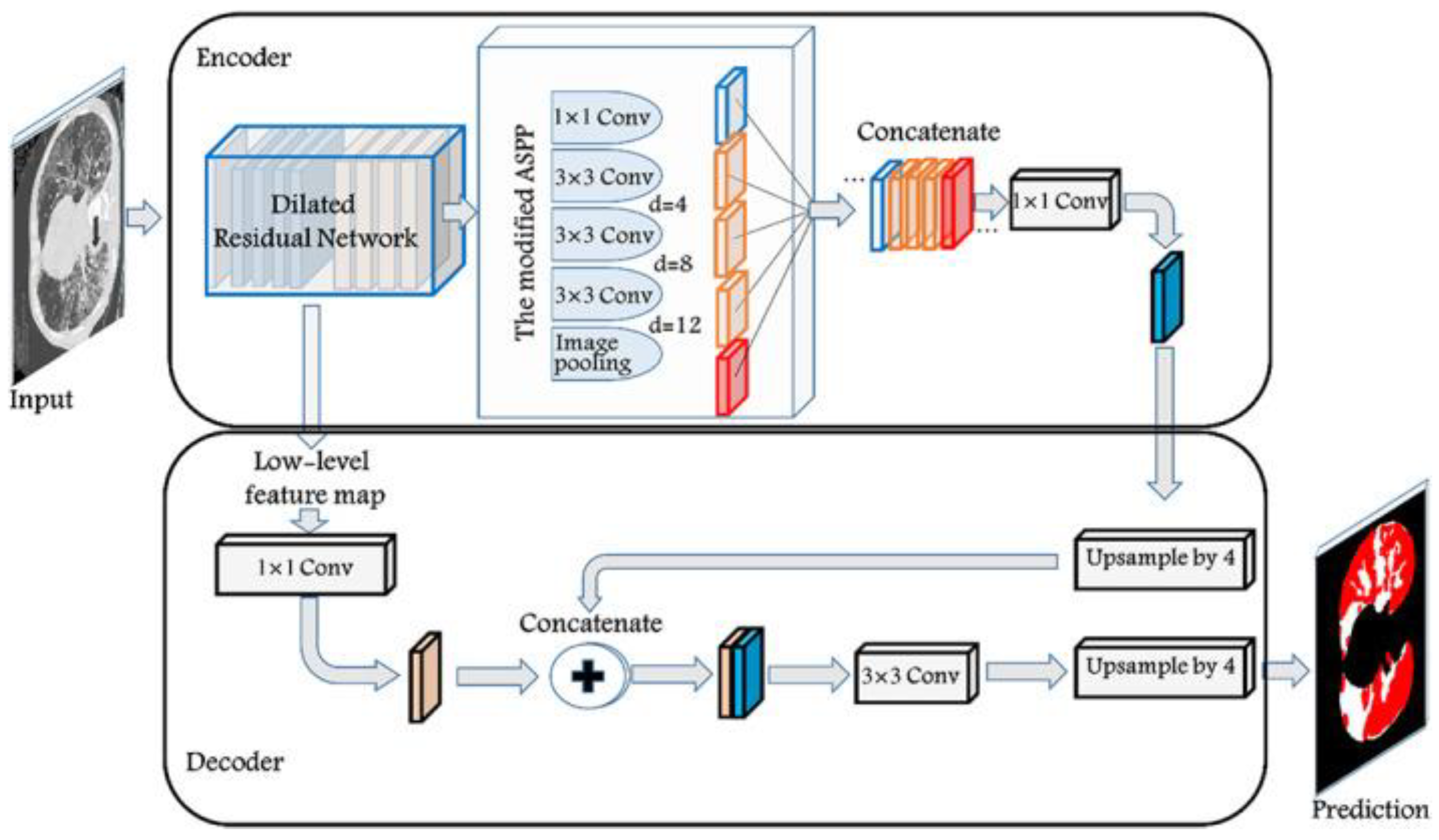
13]. The model utilizes ResNet-101 as a basic feature extractor which then gets passed on to both the decoder and the Atrous convolution pyramid shown in
Figure 5 for higher level features. The decoder concatenates the ResNet and the deeper level features while upscaling them to generate the segmentation map.
Figure 5.
DeepLabv3 full architecture.
Figure 5.
DeepLabv3 full architecture.
2.4.2. Biomarker Architecture
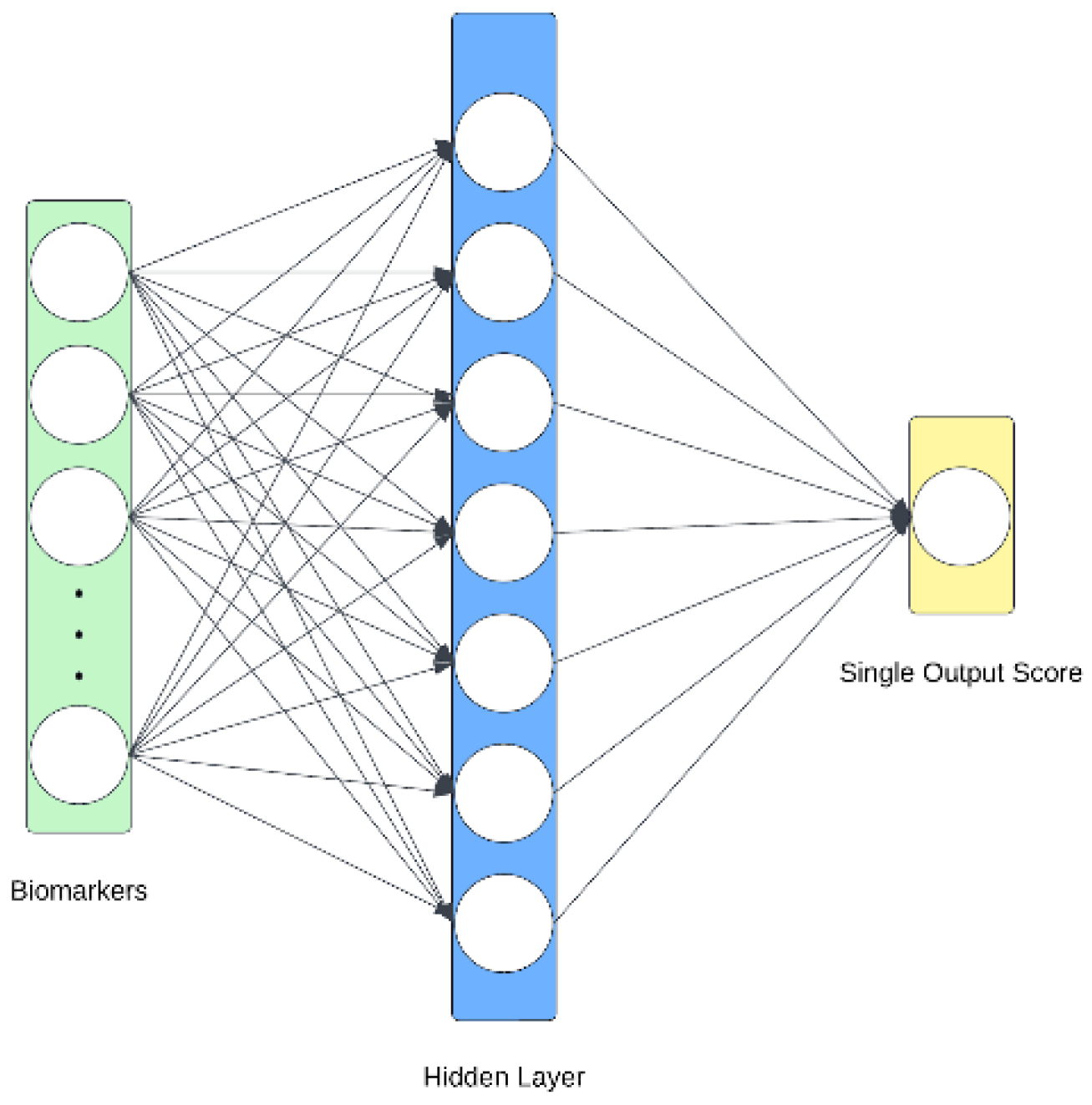
The biomarker information is passed through a multilayer perceptron (MLP) which weighs each of the 77 features and produces a singular score. This score is passed through a sigmoid to obtain a probability and ensure consistency between itself and the imaging model.
2.4.3. Multimodal Architecture
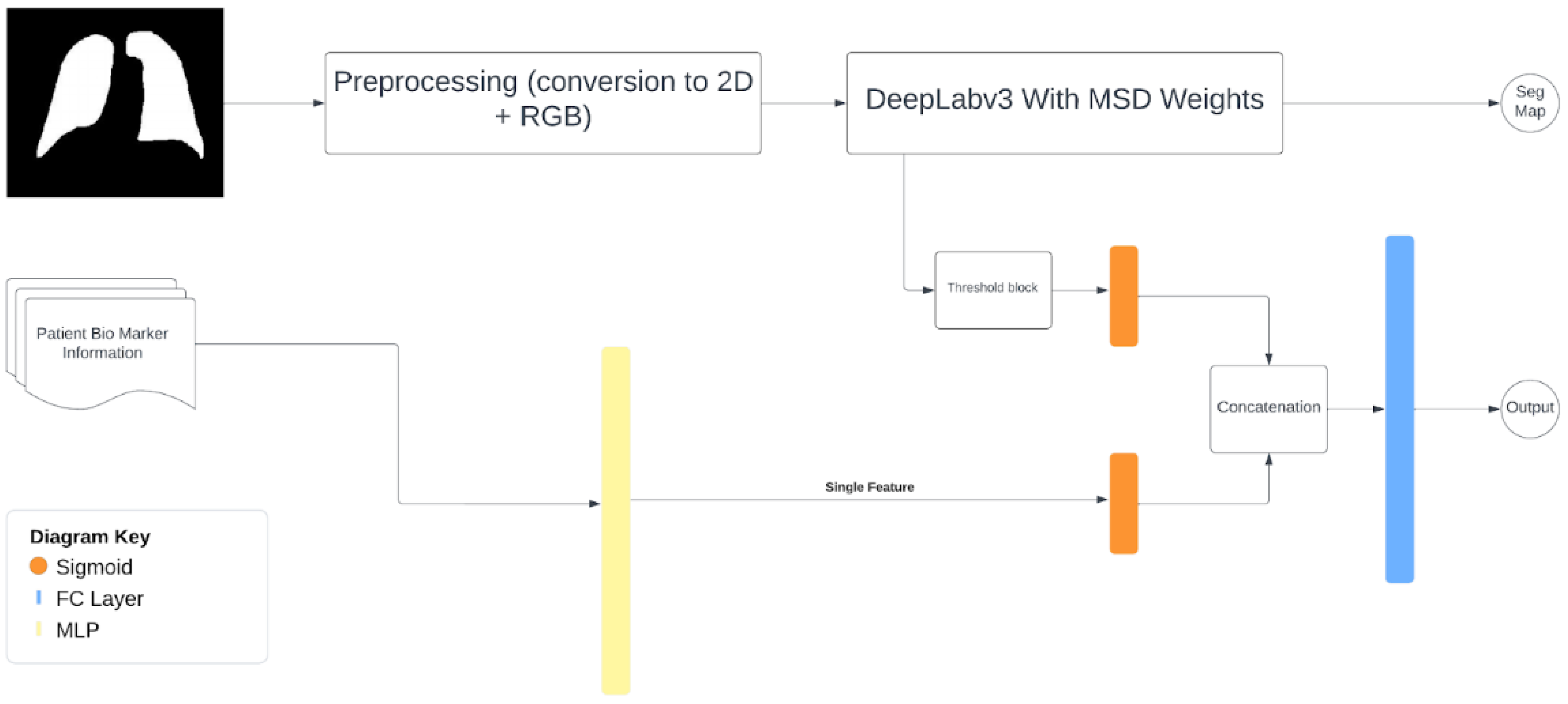
The imaging-biomarker multimodal model takes in two inputs, a probability from the imaging section and one from the biomarkers. For the imaging half, the full CT scan is used but is internally split up into slices and normalized. They are then passed to the trained version of Deeplabv3 to produce segmentation maps. The maps are then passed through a threshold system which averages the confidence of all pixels believed to be positive, which is then returned to the rest of the multimodal model. This confidence is then combined with the biomarker confidence which was simultaneously being calculated, and then passed through a fully connected layer for a single final output.
Figure 7.
Multimodal model.
Figure 7.
Multimodal model.
2.5. Model Training
Table 1.
Hardware specifications .
Table 1.
Hardware specifications .
| Part |
Specification |
| CPU |
2x vCPU |
| GPU |
Nvidia A100 40GB |
| RAM |
32 GB |
| Storage |
Google Drive |
2.5.1. Segmentation Model Training
The model was trained for twenty-five epochs with a batch size of sixteen. It used Binary-Cross-Entropy loss and Adam optimizer. A 0.80.2 cross validation was used for evaluation (1405 and 351 files respectively).
Table 2.
Segmentation model metrics .
Table 2.
Segmentation model metrics .
| Metric |
Calculation |
| Specificity |
|
| Dice Coefficient |
|
2.5.2. Multimodal Model Training
The model was trained with fifteen epochs and a batch size of four. It used Binary Cross Entropy with logits loss, Adam Optimizer with a weight decay of 1e - 5, AMSgrad active and patience of three. The model was tested on 166 set aside files from the original dataset containing 13 positive files.
Table 3.
Multimodal model metrics.
Table 3.
Multimodal model metrics.
| Metric |
Calculation |
| F1 score |
|
| Average Precision |
|
3. Results
3.1. Segmentation Results
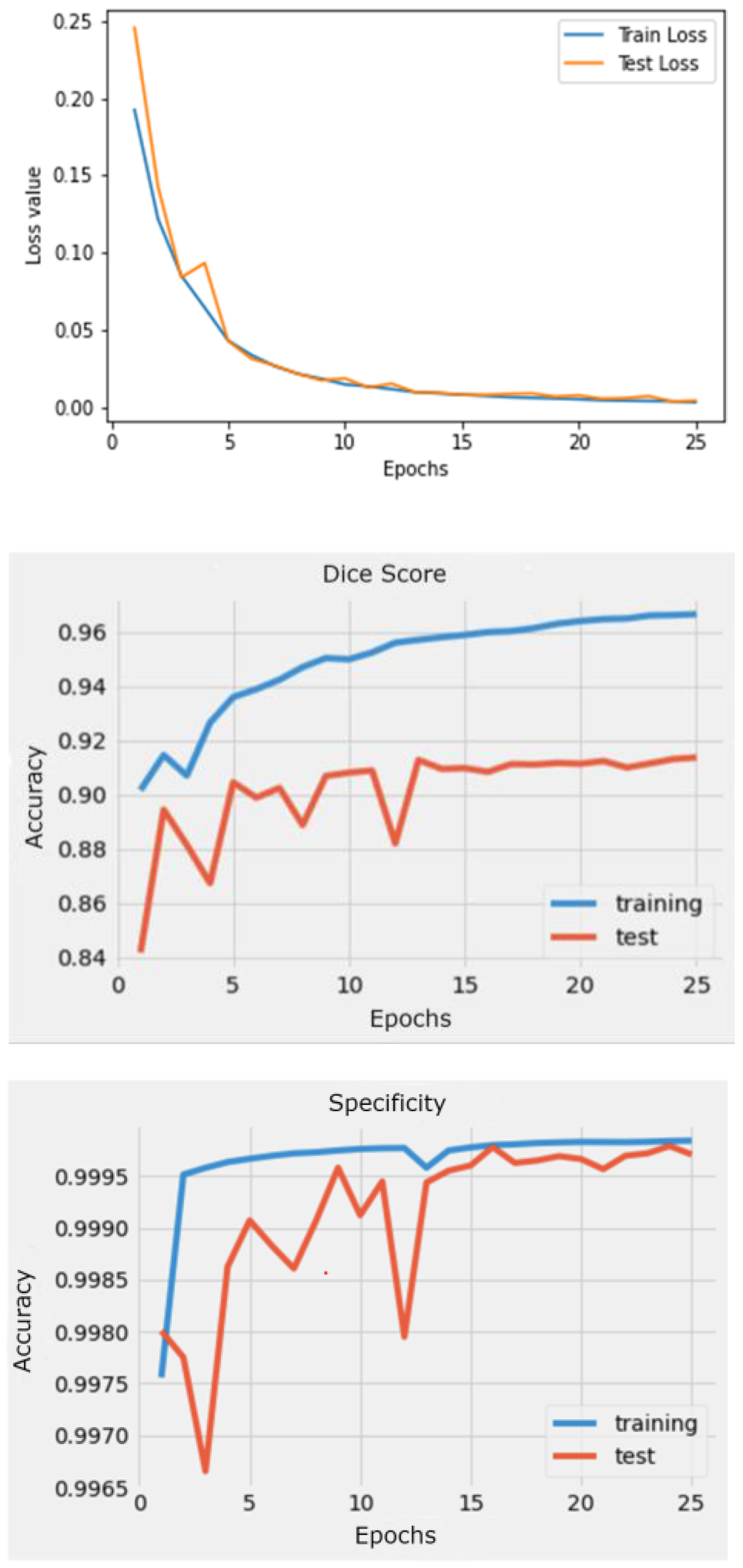
The results produced by this approach provides evidence of the accuracy of 2D segmentation compared to 3D as seen through the test DICE coefficient of 91.4%, and Specificity of 99.9%.
Figure 8.
Model Loss and metrics during training.
Figure 8.
Model Loss and metrics during training.
3.2. Multimodal Results
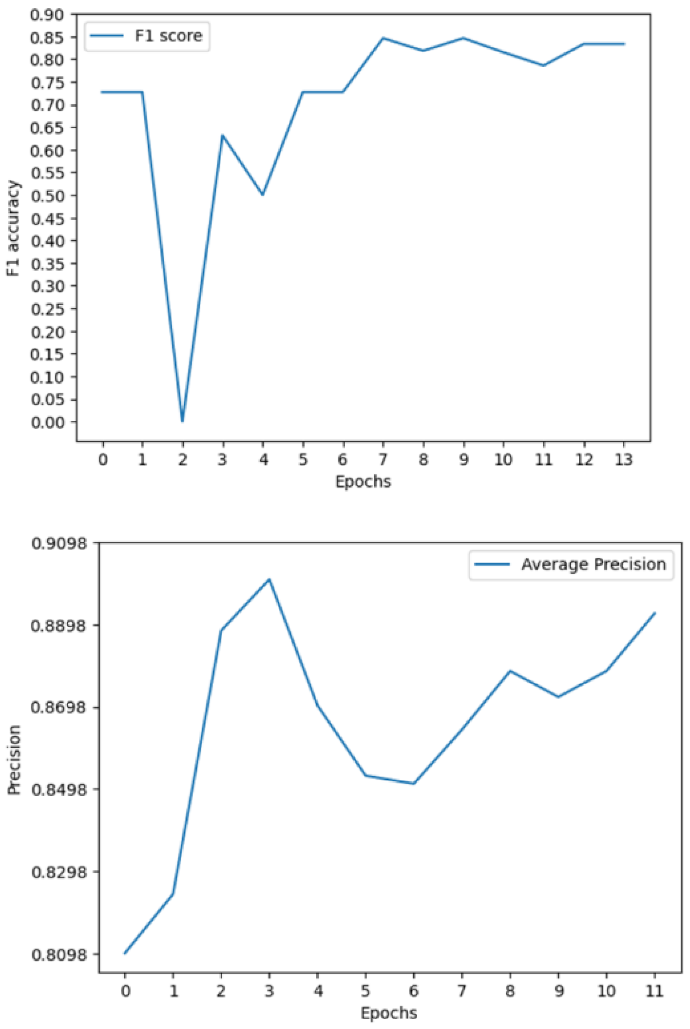
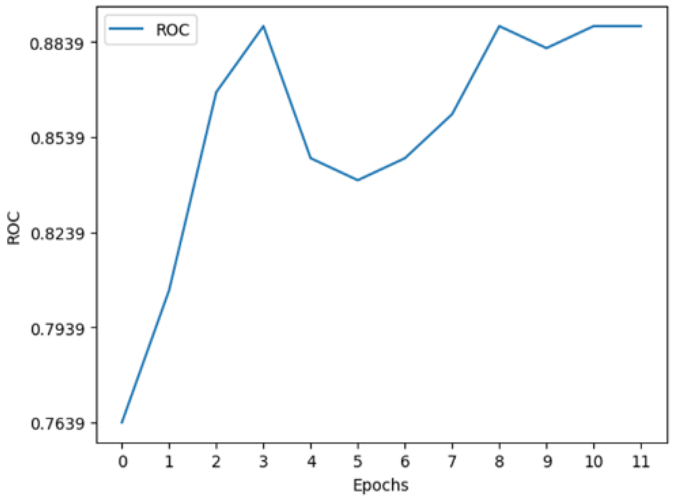
The results produced by this novel approach prove to be substantially better than the current state of the art as seen through the F1, ROC, and AP scores of 0.85, 0.89, and 0.91. These results improve on the previous state-of-the-art F1, ROC and AP by 0.45, 0.05, and 0.508 respectively.
3.3. Model Comparasion
Table 4.
Comparison of image models (general).
Table 4.
Comparison of image models (general).
| Author |
Accuracy/Dice |
Model Type |
Data Size |
| Agnes et al. |
0.83 |
3D Segmentation |
300 |
| S. Primakov et al. |
0.82 |
3D segmentation |
1328 |
| L. Daza et al. |
0.207 |
3D classification |
830 |
| S. Zhang et al. |
0.97 |
2D classification |
1018 |
| M. Roa et al. |
0.191 |
3D classification |
830 |
| Us |
0.91 |
2D segmentation |
64 |
Table 5.
Comparison of multimodal models on LUCAS.
Table 5.
Comparison of multimodal models on LUCAS.
| Author |
ROC |
Precision |
F1 |
| J. Barrett et al. |
0.847 |
0.53 |
0.508 |
| L. Daza et al. |
0.72 |
0.09 |
0.25 |
| M. Roa et al. |
- |
0.251 |
0.341 |
| Us |
0.89 |
0.91 |
0.85 |
4. Discussion
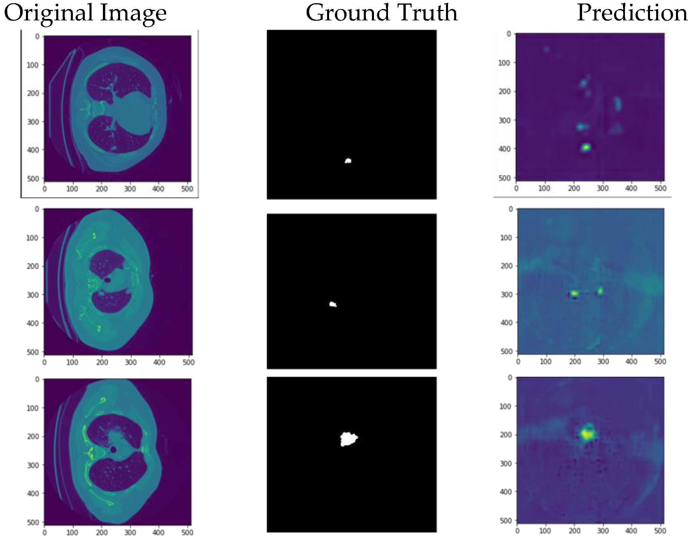
The model can accurately segment unseen and augmented data as seen in
Figure 9. The model can segment stage one tumors, indicating the system is able to handle early detection which is key. The multimodal system can perform well in testing even when put through highly imbalanced data as seen by the F1 score. The DICE coefficient for our model is higher than state-of-the-art 3D segmentation models by 0.08 (8%). The combination of a high specificity and slightly lower dice score tells us the model can accurately find all the negative pixels, while it struggles more with finding all the positive ones. The model also required much lower computational power compared to most 3D models as seen through the quicker training times. In addition, the state-of-the-art multimodal model was surpassed in F1, AUC, and precision. Specifically, with the F1 score, the state of the art was surpassed by 67.32% (0.508 to 0.85) and compared to the original baseline there was a 240% increase (0.25 to 0.85) [
8,
10]. The most important of these metrics is the F1 score which provides a more balances measure. This helps support the idea that the model will be able to function and perform in a clinical scenario where patients are at high risk and positive cases are not common.
Figure 9.
Multimodal metrics during training.
Figure 9.
Multimodal metrics during training.
Figure 10.
My model’s output on new augmented data compared to the ground truth.
Figure 10.
My model’s output on new augmented data compared to the ground truth.
Although these results are strong for a segmentation model, it is not as good as state-of-the-art classification models. But this slight drop in accuracy is acceptable when it comes to the real clinical world because the model offers justification on its output compared to the classification models. In addition, all work done is fully replicable with all data being open source, all steps of work explained, and code available upon request allowing for other authors to improve the system further. Finally, both models can always be tuned further to achieve better results.
5. Limitations
The LUCAS dataset proved to be a very challenging dataset to work with for a few reasons. First, it’s worth noting that over 350 of the patient scans contained nodules, while only 72 of them were cancer positive. It is easy for the segmentation model to misclassify a nodule as a cancerous tumor as it has not been trained to differentiate the two, leading to a highly likely decrease in the model’s performance. In addition, Daza et al. mention many of the patients were at high risk of lung cancer. This information should be reflected in the biomarkers with traits such as being a smoker presenting often. With so few positive samples but so many high-risk patients, it is easy for the biomarker comprehension part of the model to learn the wrong factors being highly correlated. This is highly possible as I found the highest correlated factor was cancer history at 0.253 while known highly correlated factors such as asthma were instead negatively correlated at -0.037. Finally, there were only 60 positive training files and 12 positive testing files. This meant that there is very low generality for the model and the results will need many more positive samples to confirm results.
6. Conclusion
Our model met the goals that we had originally set. The segmentation model output is explainable. The approach of using a 2D segmentation model vs a 3D proved beneficial for the given task. The results for both models are better or at par with comparable state-of-the-art models. Along with improvements in multimodal detection rates, this approach also improves model transparency and explainability, needed for clinical implementation. The metrics, specifically the DICE and F1 score, show promise for further improvement in the imaging-biomarker diagnostics space with this model serving as a new baseline for it. With a larger, more realistic dataset, a more advanced model architecture, and a better-fine-tuned system, results can be improved even more, turning the realm of image-biomarker based lung cancer diagnostics into a viable clinical method.
Author Contributions
Conceptualization, Pranay Kocheta; Data curation, Pranay Kocheta; Formal analysis, Pranay Kocheta; Methodology, Pranay Kocheta; Software, Pranay Kocheta; Supervision, Patrick Emedom-Nnamdi; Validation, Pranay Kocheta; Writing – original draft, Pranay Kocheta.
Funding
This research received no external funding.
Institutional Review Board Statement
Not applicable.
Informed Consent Statement
Not applicable.
Data Availability Statement
Acknowledgments
We would like to thank the creators of the MSD dataset for creating the public dataset and the authors of the LUCAS paper and dataset for taking the time to talk with us about their experience when building their model and giving their advice in addition to sharing code. I would also like to give a special thanks to Dr. Emedom-Nnamdi for helping guide me through this project.
Conflicts of Interest
I declare no conflict of interest.
References
- Rampinelli C, Origgi D, Bellomi M. Low-dose CT: technique, reading methods and image interpretation. Cancer Imaging. 2013 Feb 8;12(3):548-56. [CrossRef] [PubMed] [PubMed Central]
- Parsons AM, Ennis EK, Yankaskas BC, Parker LA Jr, Hyslop WB, Detterbeck FC. Helical computed tomography inaccuracy in the detection of pulmonary metastases: can it be improved? Ann Thorac Surg. 2007 Dec;84(6):1830-6. [CrossRef] [PubMed]
- Peuchot M, Libshitz HI. Pulmonary metastatic disease: radiologic-surgical correlation. Radiology. 1987 Sep;164(3):719-22. [CrossRef] [PubMed]
- Abdullah Muzahid, Wan, W., & Hou, L. (2020). A New Volumetric CNN for 3D Object Classification Based on Joint Multiscale Feature and Subvolume Supervised Learning Approaches. Computational Intelligence and Neuroscience, 2020, 1–17. [CrossRef]
- Kline, A., Wang, H., Li, Y. et al. Multimodal machine learning in precision health: A scoping review. npj Digit. Med. 5, 171 (2022). [CrossRef]
- Primakov, S.P., Ibrahim, A., van Timmeren, J.E. et al. Automated detection and segmentation of non-small cell lung cancer computed tomography images. Nat Commun 13, 3423 (2022). [CrossRef]
- Zhang S, Sun F, Wang N, Zhang C, Yu Q, Zhang M, Babyn P, Zhong H. Computer-Aided Diagnosis (CAD) of Pulmonary Nodule of Thoracic CT Image Using Transfer Learning. J Digit Imaging. 2019 Dec;32(6):995-1007. [CrossRef] [PubMed] [PubMed Central]
- Daza, L., Castillo, A., Escobar, M., Valencia, S., Pinzón, B., Arbeláez, P. (2020). LUCAS: LUng CAncer Screening with Multimodal Biomarkers. In: Syeda-Mahmood, T., et al. Multimodal Learning for Clinical Decision Support and Clinical Image-Based Procedures. CLIP ML-CDS 2020 2020. Lecture Notes in Computer Science(), vol 12445. Springer, Cham. [CrossRef]
- Roa, M., Daza, L., Escobar, M., Castillo, A., Arbelaez, P. (2021). SAMA: Spatially-Aware Multimodal Network with Attention For Early Lung Cancer Diagnosis. In: Syeda-Mahmood, T., et al. Multimodal Learning for Clinical Decision Support. ML-CDS 2021. Lecture Notes in Computer Science(), vol 13050. Springer, Cham. [CrossRef]
- Barrett, J.; Viana, T. EMM-LC Fusion: Enhanced Multimodal Fusion for Lung Cancer Classification. AI 2022, 3, 659-682. [CrossRef]
- Antonelli, M., Reinke, A., Bakas, S. et al. The Medical Segmentation Decathlon. Nat Commun 13, 4128 (2022). [CrossRef]
- Singh, V. (2023, November 6). Deeplabv3 & Deeplabv3+ The Ultimate Pytorch Guide. LearnOpenCV. https://learnopencv.com/deeplabv3-ultimate-guide/.
- Polat, H.: A modified DeepLabV3+ based semantic segmentation of chest computed tomography images for COVID-19 lung infections. Int. J. Imaging Syst. Technol. 32(5), 1481–1495 (2022). [CrossRef]
- Chen, L., Papandreou, G., Schroff, F., & Adam, H. (2017). Rethinking Atrous Convolution for Semantic Image Segmentation. ArXiv. /abs/1706.05587.
- Boehm, K.M., Khosravi, P., Vanguri, R. et al. Harnessing multimodal data integration to advance precision oncology. Nat Rev Cancer 22, 114–126 (2022). [CrossRef]
- Geert Litjens, Kooi, T., Babak Ehteshami Bejnordi, Arnaud, Ciompi, F., Mohsen Ghafoorian, van, Bram van Ginneken, & Sánchez, C. I. (2017). A survey on deep learning in medical image analysis. Medical Image Analysis, 42, 60–88. [CrossRef]
- Merino, I., Azpiazu, J., Remazeilles, A., & Sierra, B. (2021). 3D Convolutional Neural Networks Initialized from Pretrained 2D Convolutional Neural Networks for Classification of Industrial Parts. Sensors, 21(4), 1078. [CrossRef]
- Yu, J., Yang, B., Wang, J., Leader, J., Wilson, D., & Pu, J. (2020). 2D CNN versus 3D CNN for false-positive reduction in lung cancer screening. Journal of Medical Imaging, 7(05). [CrossRef]
- Ali Ahmed, S. A., Yavuz, M. C., Şen, M. U., Gülşen, F., Tutar, O., Korkmazer, B., Samancı, C., Şirolu, S., Hamid, R., Eryürekli, A. E., Mammadov, T., & Yanikoglu, B. (2022). Comparison and ensemble of 2D and 3D approaches for COVID-19 detection in CT images. Neurocomputing, 488, 457–469. [CrossRef]
- Geert Litjens, Kooi, T., Babak Ehteshami Bejnordi, Arnaud, Ciompi, F., Mohsen Ghafoorian, van, Bram van Ginneken, & Sánchez, C. I. (2017). A survey on deep learning in medical image analysis. Medical Image Analysis, 42, 60–88. [CrossRef]
- Boehm, K.M., Aherne, E.A., Ellenson, L. et al. Multimodal data integration using machine learning improves risk stratification of high-grade serous ovarian cancer. Nat Cancer 3, 723–733 (2022). [CrossRef]
- Zhang, G., Yang, Z. & Jiang, S. Automatic lung tumor segmentation from CT images using improved 3D densely connected UNet. Med Biol Eng Comput 60, 3311–3323 (2022). [CrossRef]
- Agnes SA, Anitha J. Efficient multiscale fully convolutional UNet model for segmentation of 3D lung nodule from CT image. J Med Imaging (Bellingham). 2022 Sep;9(5):052402. Epub 2022 May 11. [CrossRef] [PubMed] [PubMed Central]
- Singh, S.P.; Wang, L.; Gupta, S.; Goli, H.; Padmanabhan, P.; Gulyás, B. 3D Deep Learning on Medical Images: A Review. Sensors 2020, 20, 5097. [CrossRef]
- Yu, H., Li, J., Zhang, L. et al. Design of lung nodules segmentation and recognition algorithm based on deep learning. BMC Bioinformatics 22 (Suppl 5), 314 (2021). [CrossRef]
- Voigt, W.; Prosch, H.; Silva, M. Clinical Scores, Biomarkers and IT Tools in Lung Cancer Screening—Can an Integrated Approach Overcome Current Challenges? Cancers 2023, 15, 1218. [CrossRef]
|
Disclaimer/Publisher’s Note: The statements, opinions and data contained in all publications are solely those of the individual author(s) and contributor(s) and not of MDPI and/or the editor(s). MDPI and/or the editor(s) disclaim responsibility for any injury to people or property resulting from any ideas, methods, instructions or products referred to in the content. |
© 2024 by the authors. Licensee MDPI, Basel, Switzerland. This article is an open access article distributed under the terms and conditions of the Creative Commons Attribution (CC BY) license (http://creativecommons.org/licenses/by/4.0/).
