1. Introduction
The thermal history of matter plays a crucial role in various thermomechanical processes, particularly in additive manufacturing. In this context, the material undergoes multiple diverse thermal loads, resulting in complex microstructures that significantly impact the performance of manufactured parts [
1,
2,
3]. Real-time prediction of microstructures is essential in the context of the digital twin, as it enhances manufacturing process performance [
4]. Traditional numerical models based on classical methods (finite elements, finite volumes, finite difference) face limitations in terms of prediction speed [
5]. To overcome these limitations, substitution models such as neural networks, especially Physics-Informed Neural Networks (PINNs), have been employed. PINNs integrate the system’s physical equations into the learning process and have gained popularity since the work of Raissi et al. in 2019, with numerous studies and dedicated libraries emerging. Despite their advantages, PINNs encounter convergence issues that are often treated on a case-by-case basis.
The challenges of PINNs are further compounded by the intricate nature of the additive manufacturing process. This process is not only costly and difficult to model but also presents specific challenges for PINNs related to the dynamic changes in the part’s geometry during production. The significant variability of part geometries in Laser Powder Bed Fusion (LPBF) almost necessitates the development of a separate model for each part. Nevertheless, leveraging insights from the literature can help develop approaches to address some of these challenges. For instance, managing geometry changes can be achieved using PINNs based on convolutional neural networks (CNN) or utilizing PointNets, as suggested by [
6].
This project aims to simulate real-time additive manufacturing based on the multi-scale approach proposed by [
7] for thermal modeling of LPBF. The objective is to create a robust physics-informed neural network (PINN) as a substitute for finite element models. By addressing complexities and convergence issues, we propose in this paper a reliable method demonstrated on a 2D transient problem—a crucial step for achieving real-time LPBF simulation using PINNs. The approach can be coupled with nearly all strategies used to enhance the convergence of PINNs.
2. Modeling and Methods
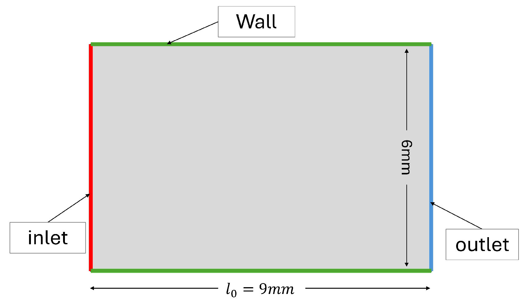
The model’s geometry is illustrated in
Figure 1. The method involves appropriately scaling the network and weighting physical equations, initial conditions, and boundary conditions. The transient diffusion partial differential equation (PDE) is expressed as follows:
Where material properties include density , specific heat , and thermal conductivity .
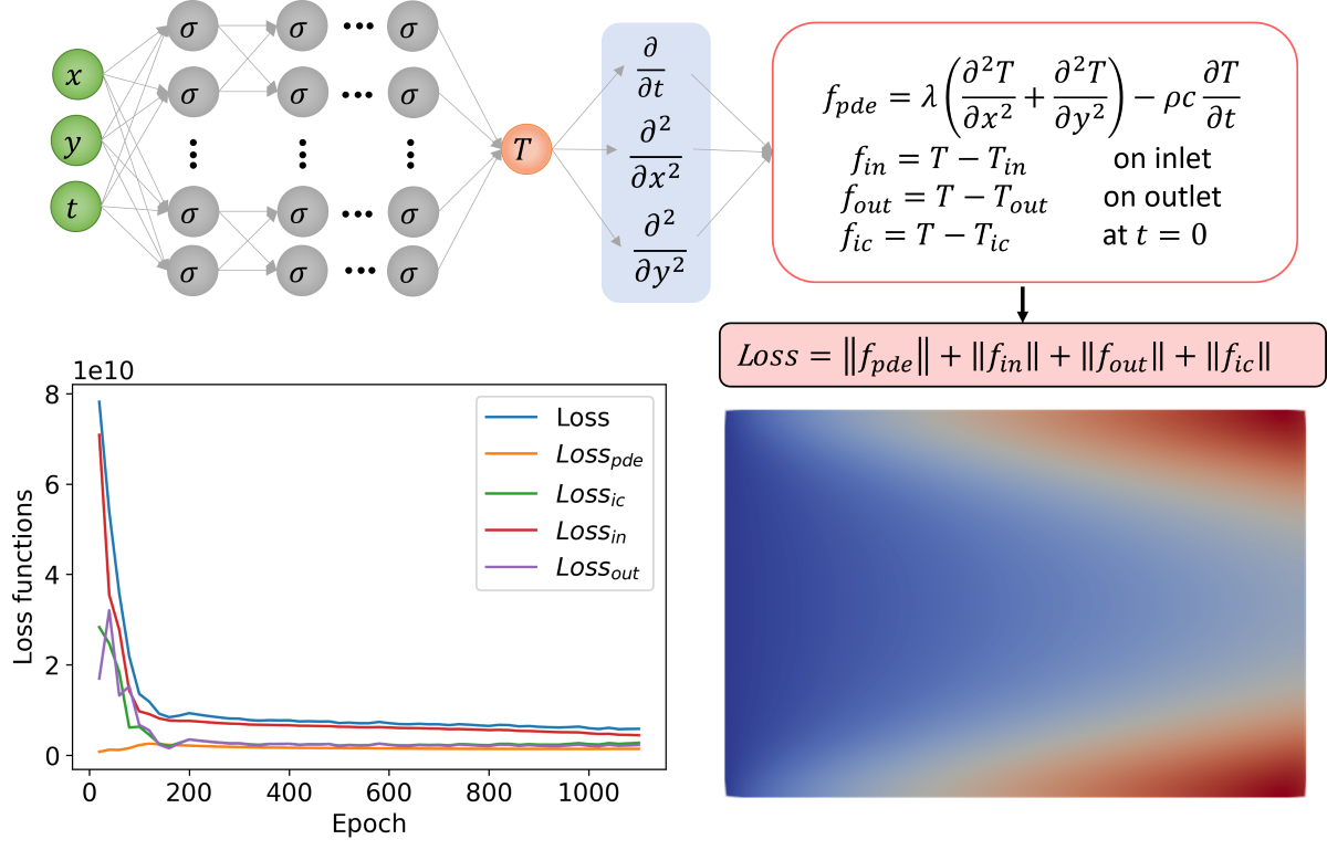
The architecture of the PINN network is depicted in
Figure 2.
To assess the network’s robustness, various configurations will be tested. The first group focuses on models with Dirichlet boundary conditions, while the second group involves both Dirichlet and Fourier boundary conditions (convective exchange boundary conditions with the external environment). The third group uses the same conditions as the second group but includes an advection phenomenon.
Throughout the document, the ADAM optimization algorithm is used, testing the robustness of this approach against the commonly recommended L-BFGS algorithm for PINNs [
8,
9]. Results from PINNs will be compared with numerical models developed using the finite element code Abaqus to validate predictions.
3. Problem with Exclusive Use of Dirichlet Boundary Conditions
The model’s configuration and the delineation of the outlet and inlet boundaries are depicted in
Figure 1. The dimensions of the plate are
in length and
in width. At the inlet and outlet, temperatures
and
are prescribed, respectively. The initial temperature is set to
, and the total physical simulation time is
. With these conditions, the diffusion thermal problem is surely constant along the y-direction, so it is not necessary to impose a boundary condition on the wall boundary of the domain.
In the context of Problem
1, where only Dirichlet boundary conditions are employed, the operator
B functions as an identity,
denotes the temperature imposed at the domain boundary, and the equations are redefined as follows:
Introducing residuals denoted as
R, we define:
To normalize the network by making its inputs and outputs dimensionless, we adopt reference quantities such as temperature
, the length
of the model geometry, and the time
. The new dimensionless variables are expressed as:
,
,
, and
. Utilizing these new variables, the physical equation transforms into:
Consequently, the dimensionless equation is derived as:
The Root Mean Square Error (RMSE) of the residuals is expressed as:
While the conventional approach uses dimensionless loss functions
6, our method multiplies them by coefficients to bring them to a comparable scale. Hence, the loss functions are articulated as:
where
represents the model’s time increment.
Indeed, we express the PDE loss function in units of specific power and convert the loss functions for the boundary and initial conditions into the same unit. This is done by transforming the prediction error into the numerical derivative of temperature with respect to time (), and then multiplying the result by the specific heat c to obtain a quantity in units of specific power. In other words, we convert the losses from the boundary and initial conditions into a form that is equivalent to the transient term in the PDE loss. Hereafter, we will refer to the PINN using our approach as W-PINN (W for weighted).
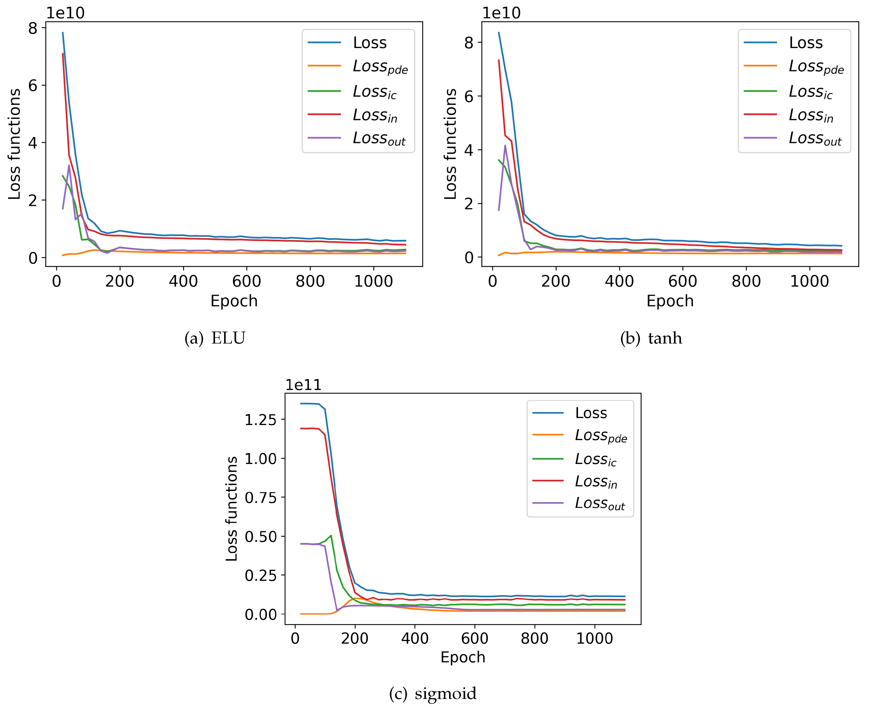
In this section, only the W-PINN model will be used to test different activation functions. The model was trained for 1100 epochs with a network comprising 6 hidden layers of 40 neurons each. The ADAM optimization algorithm was used, along with various activation functions such as Exponential Linear Unit (ELU), sigmoid, and tanh. It is worth noting that in numerical simulation, boundary conditions are forcefully applied in the initial increment. To replicate this with neural networks, the initial increment would need to be divided into multiple steps to accurately describe this evolution. For simplicity, all boundary conditions are linearly applied from the initial value to the imposed value throughout the entire simulation duration. All computations on neural networks were performed on an NVIDIA A100-PCIE-40GB GPU server. The computation times are similar, averaging about 3 minutes.
The
Figure 3 shows the loss functions for various activation functions. For the ELU and tanh activation functions (
Figure 3a,b, the evolution of the loss functions is nearly identical. At the beginning of the epochs, the outlet loss function (
) rises and then falls, indicating competition between the terms of the main loss function (
). For the sigmoid activation function (
Figure 3c), there is a plateau for about 80 epochs before the loss functions start to decrease significantly, except for the initial conditions loss function (
) and the physical equation loss function (
), which rise moderately before falling, also indicating competition between the different terms of the main loss function (
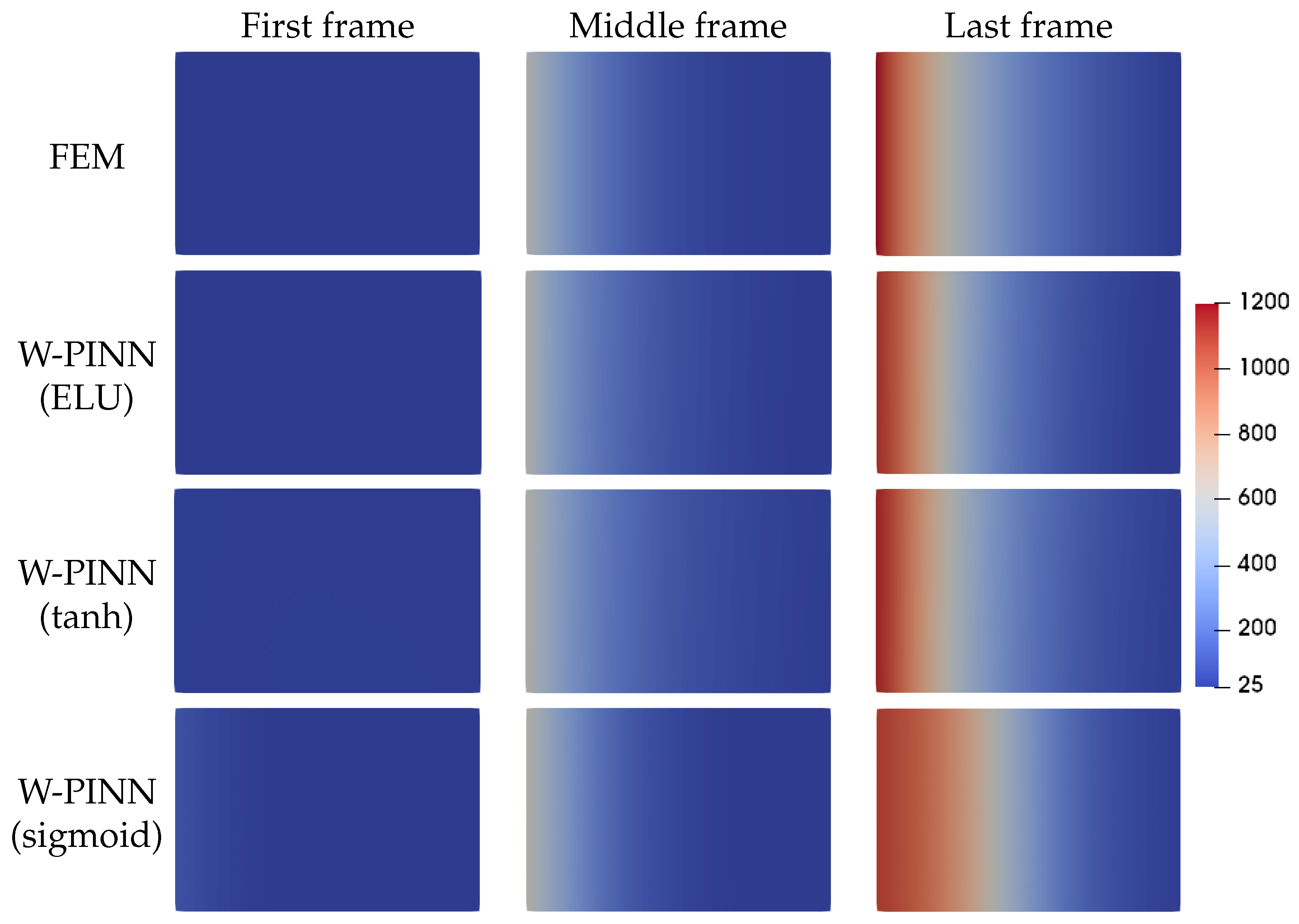
). Overall, the loss functions for each activation function converge, with the convergence being most effective for the tanh activation function, followed by the ELU function. The temperature field of the W-PINN model was compared with that of the numerical simulation, as illustrated in
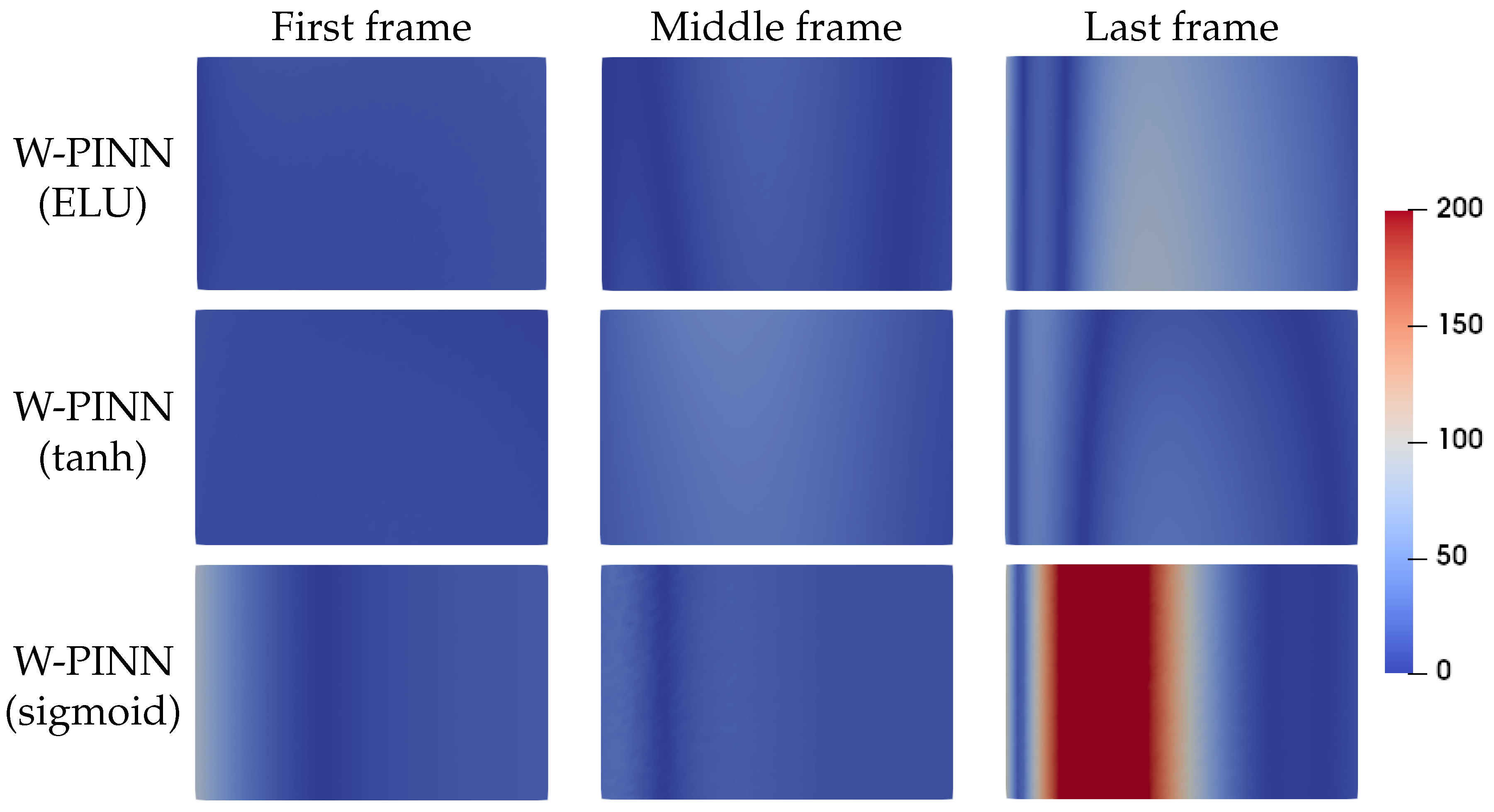
Figure 4. The initial, middle, and final frames are displayed for various activation functions. The predictions appear satisfactory except for the final frame with the sigmoid function.
To gain further insights, outputs of the absolute error of the thermal field are depicted in
Figure 5, revealing significant discrepancies between predictions of the model using the sigmoid activation function and numerical results. Several case studies have highlighted limitations of the sigmoid function compared to ELU and tanh. Therefore, it will not be used further in this document.
4. Problem with Dirichlet and Fourier Boundary Conditions
The multi-scale LPBF additive manufacturing model proposed by [
7] simulates FSW welding across various scales, considering the influence of the surrounding powder through Fourier boundary conditions. In addition to incorporating these boundary conditions into the model, we start with a warm initial condition of
to simulate the cooling of the workpiece during additive manufacturing. A Fourier boundary condition is applied at the outlet, while a Dirichlet boundary condition of linear cooling to
is applied at the inlet. The external temperature
for the Fourier boundary condition is set to decrease from
to
in accordance with the previously mentioned rule for the progressive application of boundary conditions. To create a more complex situation, a deliberately high wall heat transfer coefficient of
is used. Subsequently, we adjust the expression of the outlet loss function, which takes the form of:
We retained the architecture of the previous network but used only ELU and tanh activation functions, training for 100000 epochs. Both the proposed W-PINN method and the standard PINN method were simulated, with similar computation times averaging about 140 minutes.
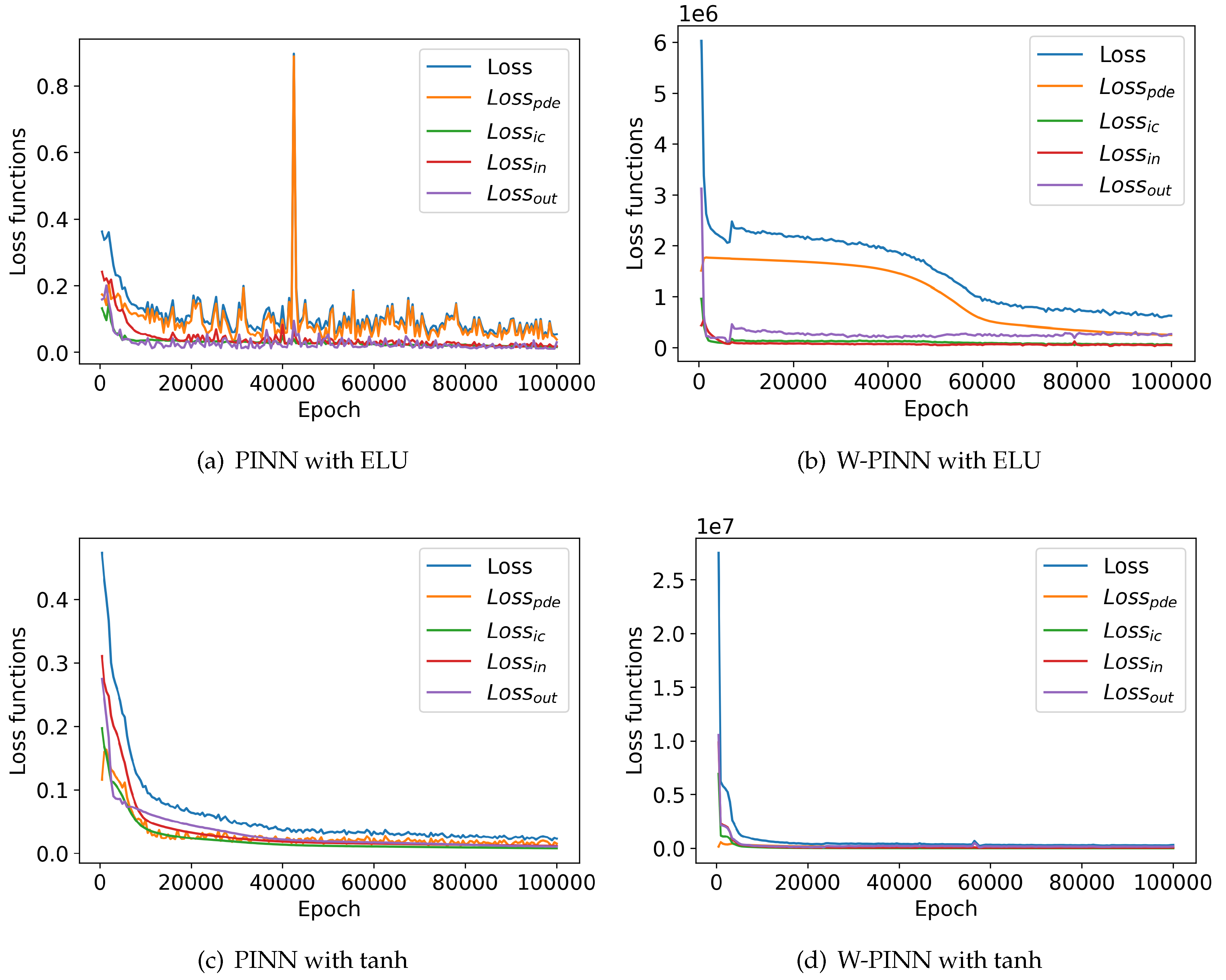
As shown in
Figure 6a,b the loss functions clearly indicate a convergence issue with the ELU activation function. With the standard PINN method (
Figure 6b), we observe instability in the functions, with a significant spike in the
function after
epochs. Additionally, the difference between the loss functions values at the beginning and the end of the epochs is not substantial. Conversely, with the proposed W-PINN approach, after an initial rapid decline, there is a slow decline or plateau, followed by a second rapid decline, resulting in much lower values at the end of the epochs compared to the beginning. Additionally, the functions are smoother and more monotonic. For the tanh activation function shown in
Figure 6c,d, the W-PINN model also shows good convergence.
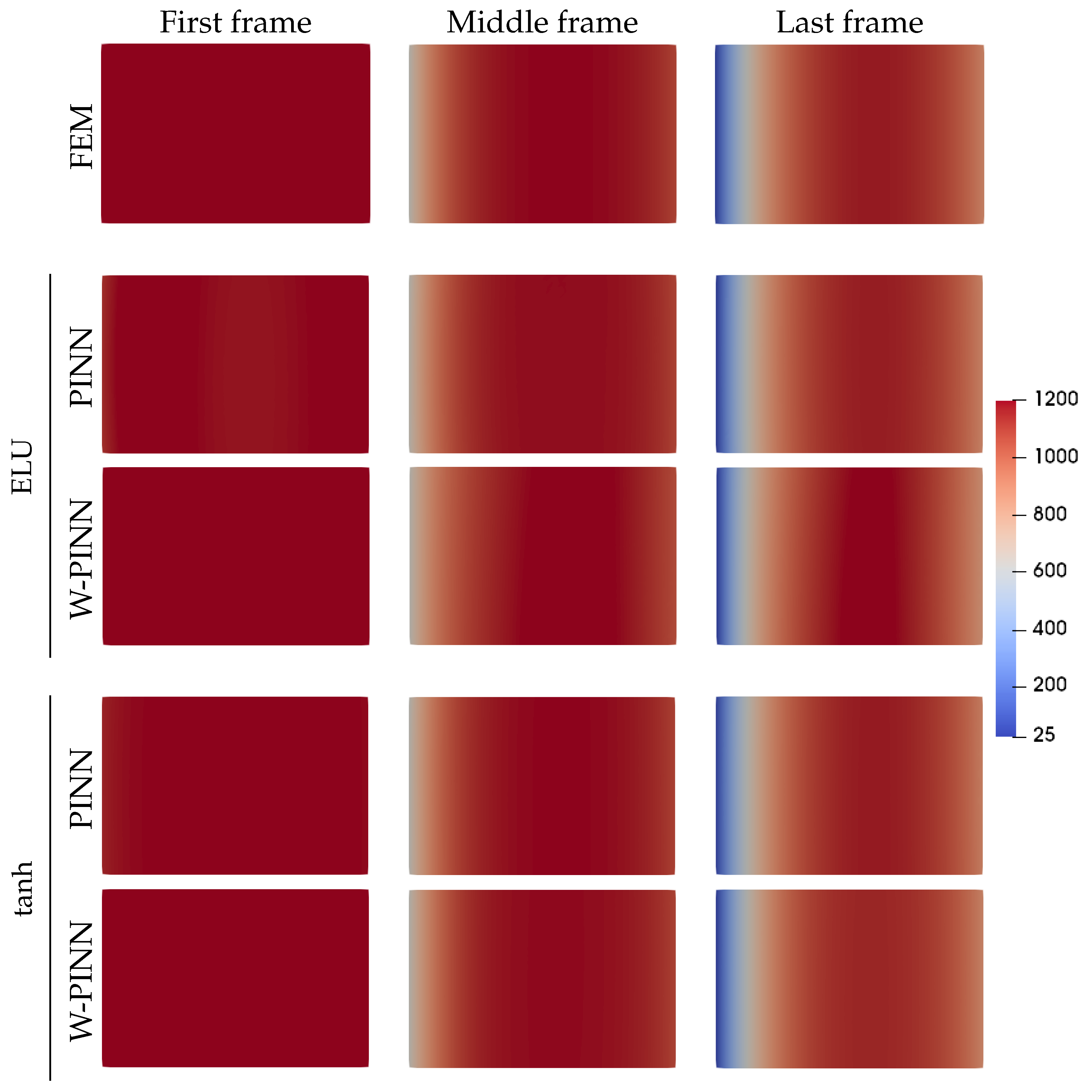
When observing the predicted temperature fields in
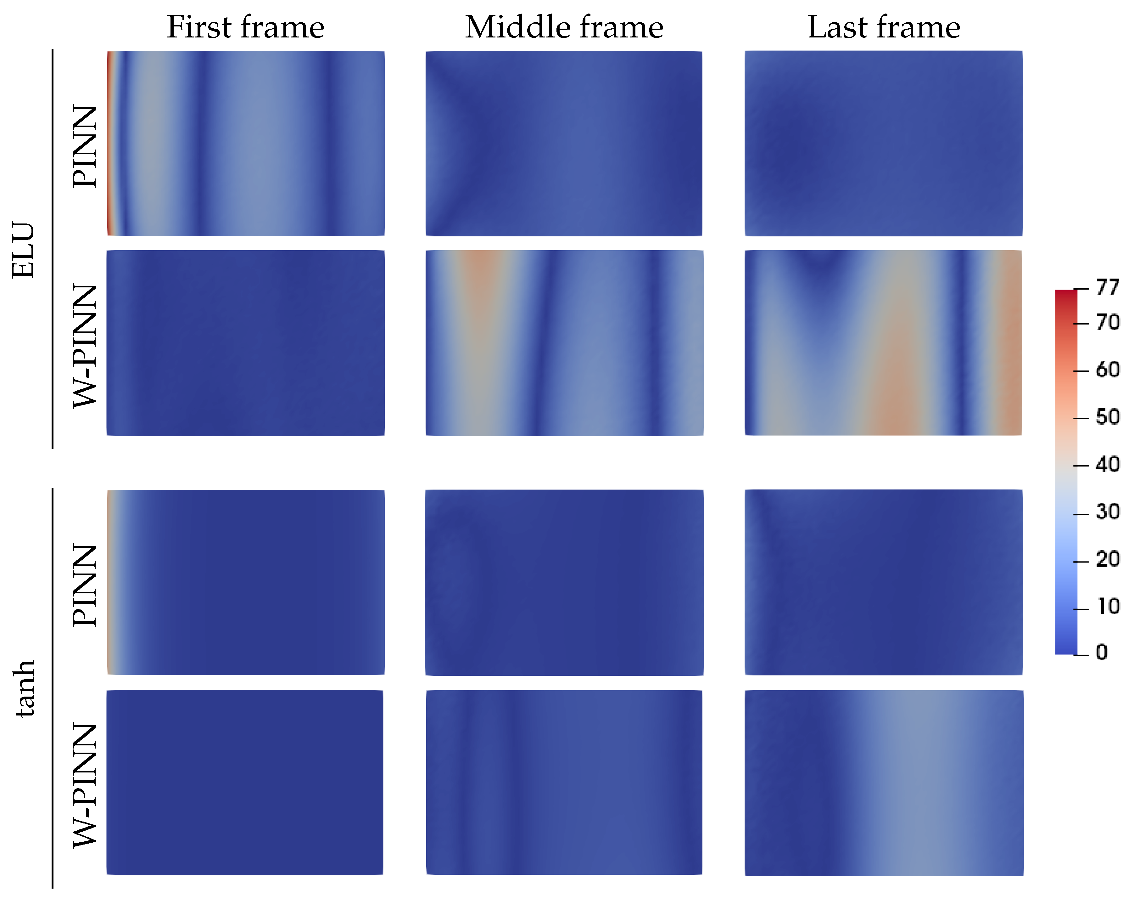
Figure 7, the results seem to align with the finite element simulation. In the final frame, it is evident that the target temperature of 25°C imposed on the inlet boundary has been successfully achieved. Additionally, the Fourier boundary condition applied at the outlet boundary has resulted in a vertical red band of higher temperatures centered along the x-direction. However, it is difficult to compare the neural network models with each other based on these visualizations. Therefore, the absolute error of the temperature field is investigated in
Figure 8. This visualization confirms that the ELU activation function yields poorer results. It can also be observed that the largest errors are located at the inlet edge of the domain. However, regarding the activation function tanh, the W-PINN model produces better results at the initial frame than the PINN model which performs better at the middle and final frames.
Furthermore,
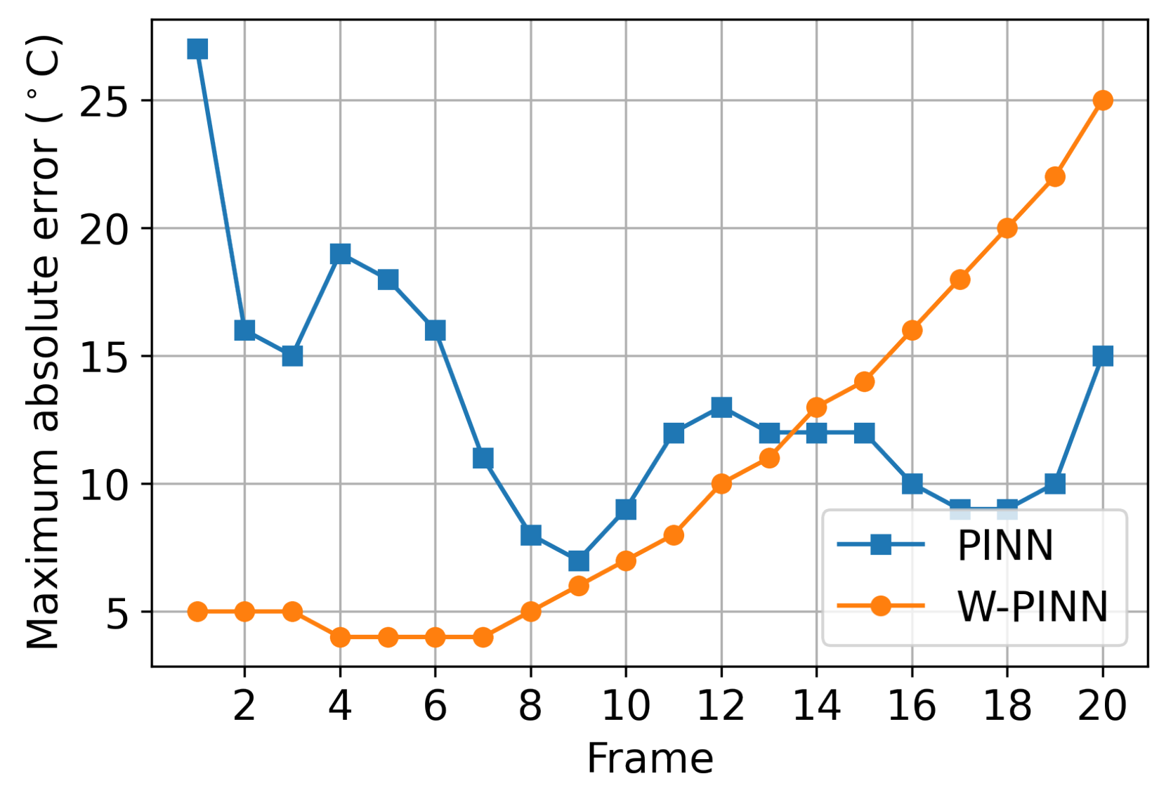
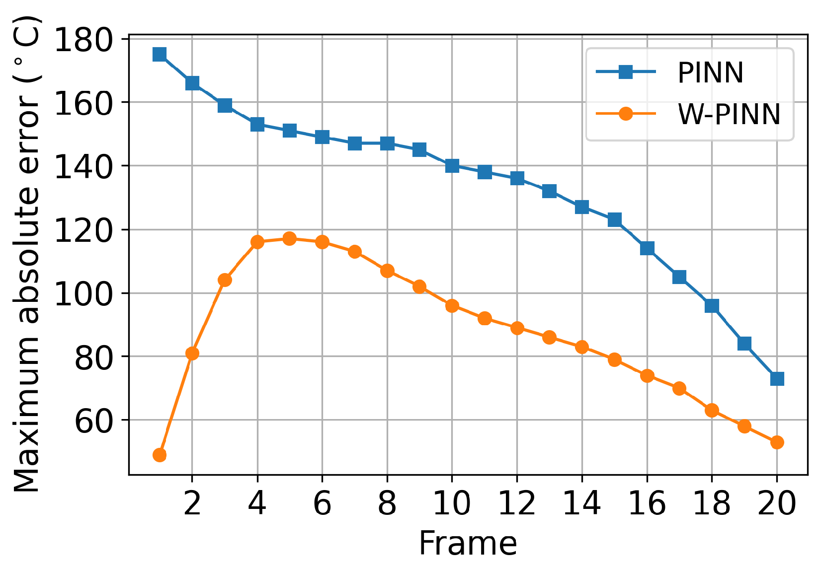
Figure 9 demonstrates that the W-PINN model also performs well on the frames following the initial frame. Analyzing all frames, we observe that the first half is well-predicted by W-PINN, while the second half is better-predicted by PINN. This is reflected in the maximum error curve of the predicted temperature field by both approaches, as shown in
Figure 10. Given the appearance of the two curves, we can conclude that the W-PINN method is generally more effective, as its maximum error value is lower than that of the PINN for 13 out of the 20 frames. Moreover, where the W-PINN’s error is higher, the difference from the PINN is not significant.
5. Problem with Advection, Dirichlet and Fourier Boundary Conditions
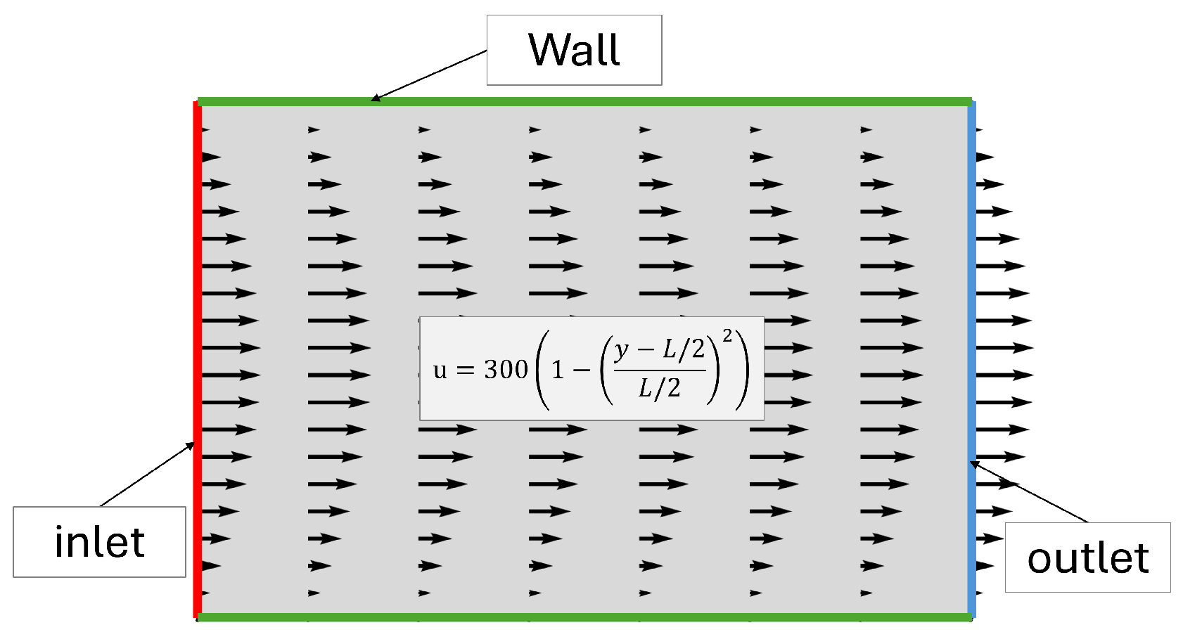
In additive manufacturing, one might be interested in the flow of material in the context of laser melting modeling, powder spreading, gas movement inside the chamber, exit velocities, and material spreading during DED-type AM processes. Generally, the flow is modeled using an Eulerian formulation and the problem is solved numerically. Sometimes, it is possible to bypass the complexity of numerical approaches by assuming the material flow based on known principles. In such cases, only the thermal problem is solved numerically, with an advection term accounting for material movement. This means that thermal advection can be utilized in many thermal problems in fluid mechanics and even in solid mechanics where the Eulerian formulation is used. In this section, advection has been incorporated into the previous problem. The imposed parabolic advection velocity field is shown in
Figure 11.
The PDE loss function becomes:
With the parabolic velocity field, the diffusion thermal problem is no more constant in y-direction. Therefore, a boundary condition of zero heat flux across the wall is imposed. It is given by:
It should be noted that for this boundary condition, we multiply the factor
by the dimensionless temperature gradient
, whereas for the others, it is multiplied by the dimensionless temperature error. This expression (Equation
10) can be improved, but here we rely on the fact that the scale does not change since the gradient
is dimensionless.
We retained the same network architecture, using only the tanh activation function and training for
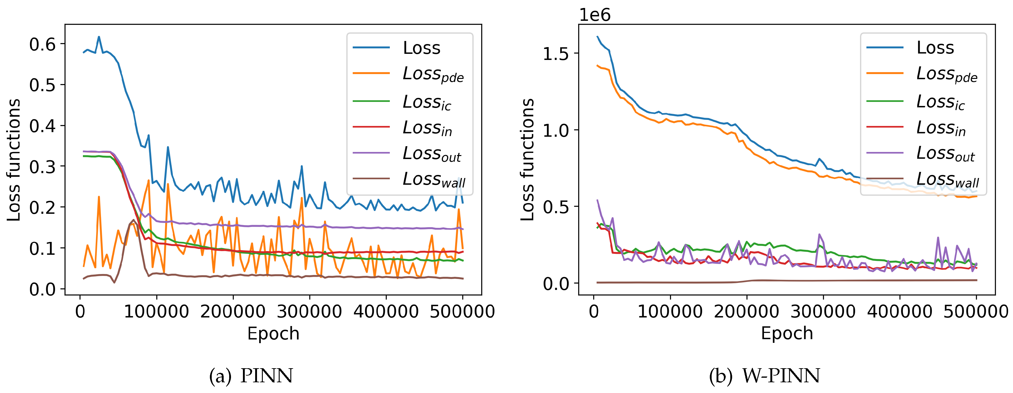
epochs. The computation times for the PINN and W-PINN models are 14 hours and 11 hours, respectively. The results of the loss function evolution are displayed in
Figure 12. For the PINN method, there is a fluctuation in the losses of the physical equation (
). Throughout the epochs,
fluctuates around the same value, indicating a lack of convergence. It is important to note that the graph does not represent the initial epochs values, which typically have values significantly different from those shown. This exclusion is made to ensure readable curves. Additionally, the losses are dominated by
for the PINN method, whereas for the W-PINN method,
is more prominent. The W-PINN model shows a more pronounced convergence, with its curve continuing to decline.
In
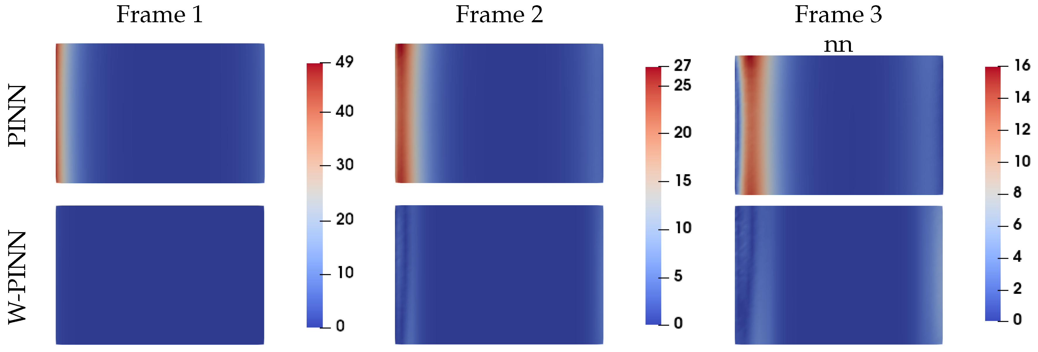
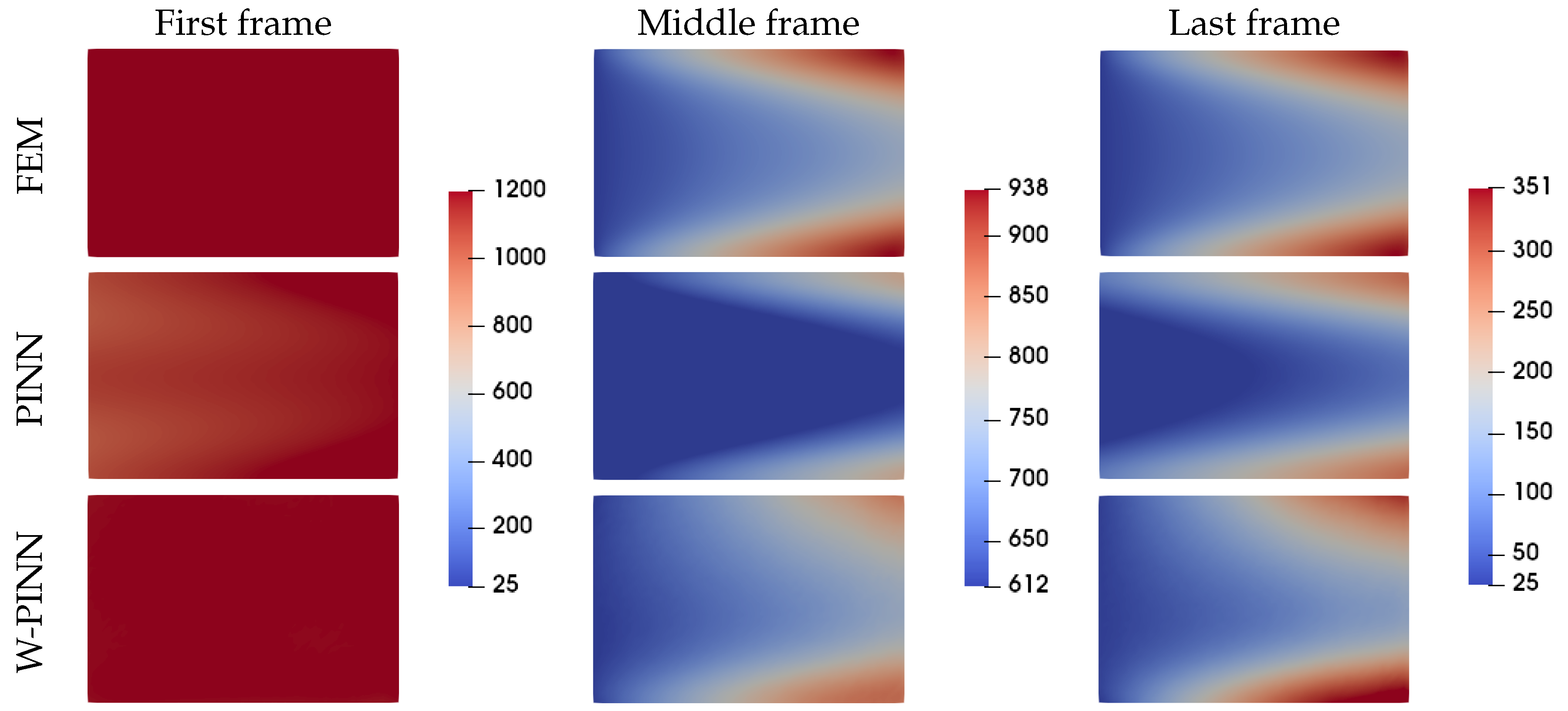
Figure 13, which depicts the temperature fields, notable differences can be observed. The PINN model is less predictive across the three frames: the first frame is characterized by two bright bands indicating temperatures around 900
, while the middle and last frames show a more intense horizontal blue cone, corresponding to a temperature of
. The maximum error curve for the thermal field, shown in the
Figure 14, clearly indicates that the W-PINN approach provides significantly better predictions than the PINN approach. In conclusion, the W-PINN approach is very straightforward and yields better results for all the cases studied. However, its speed advantage over the PINN approach in problems involving convection remains to be verified.
6. Conclusions
In this study, we explored the performance of Physics-Informed Neural Networks (PINNs) and their variant, Weighted PINNs (W-PINNs), in modeling thermal problems, incorporating various boundary conditions and flow dynamics.
W-PINNs significantly outperformed standard PINNs in terms of convergence and accuracy when applied to problems with Fourier and Dirichlet boundary conditions. W-PINNs demonstrated smoother and more consistent convergence, with lower final loss values and better alignment with finite element model predictions. When integrating advection into the thermal problem, PINNs faced challenges with convergence, particularly in maintaining stable loss values over training epochs. W-PINNs, on the other hand, showed superior performance in handling the added complexity of advection, with more pronounced convergence and lower maximum error values.
Furthermore, the W-PINN model consistently provided more accurate temperature field predictions across different activation functions, including ELU and tanh, particularly in scenarios involving complex boundary conditions and material advection. This indicates that W-PINNs are generally more reliable and effective for modeling industrial processes.
In conclusion, W-PINNs offer a robust and efficient alternative to standard PINNs for complex thermal problems. Their superior convergence behavior and accuracy make them a promising tool for advanced simulation tasks involving varying boundary conditions and flow dynamics.
References
- Gao, S.; Li, Z.; Petegem, S.V.; Ge, J.; Goel, S.; Vas, J.V.; Luzin, V.; Hu, Z.; Seet, H.L.; Sanchez, D.F.; et al. Additive manufacturing of alloys with programmable microstructure and properties. Nature Communications 2023, 14, 6752. [Google Scholar] [CrossRef] [PubMed]
- Bajaj, P.; Hariharan, A.; Kini, A.; Kürnsteiner, P.; Raabe, D.; Jägle, E.A. Steels in additive manufacturing: A review of their microstructure and properties. Materials Science and Engineering: A 2020, 772, 138633. [Google Scholar] [CrossRef]
- Delahaye, J.; Tchuindjang, J.T.; Lecomte-Beckers, J.; Rigo, O.; Habraken, A.M.; Mertens, A. Influence of Si precipitates on fracture mechanisms of AlSi10Mg parts processed by Selective Laser Melting. Acta Materialia 2019, 175, 160–170. [Google Scholar] [CrossRef]
- Aymerich, E.; Pisano, F.; Cannas, B.; Sias, G.; Fanni, A.; Gao, Y.; Böckenhoff, D.; Jakubowski, M. Physics Informed Neural Networks towards the real-time calculation of heat fluxes at W7-X. Nuclear Materials and Energy 2023, 34, 101401. [Google Scholar] [CrossRef]
- Pauza, J.G.; Tayon, W.A.; Rollett, A.D. Computer simulation of microstructure development in powder-bed additive manufacturing with crystallographic texture. Modelling and Simulation in Materials Science and Engineering 2021, 29, 055019. [Google Scholar] [CrossRef]
- Kashefi, A.; Mukerji, T. Physics-informed PointNet: A deep learning solver for steady-state incompressible flows and thermal fields on multiple sets of irregular geometries. Journal of Computational Physics 2022, 468. [Google Scholar] [CrossRef]
- Bresson, Y.; Tongne, A.; Baili, M.; Arnaud, L. Global-to-local simulation of the thermal history in the laser powder bed fusion process based on a multiscale finite element approach. International Journal of Advanced Manufacturing Technology 2023, 127, 4727–4744. [Google Scholar] [CrossRef]
- Lou, Q.; Meng, X.; Karniadakis, G.E. Physics-informed neural networks for solving forward and inverse flow problems via the Boltzmann-BGK formulation. Journal of Computational Physics 2021, 447, 110676. [Google Scholar] [CrossRef]
- Pratama, D.A.; Abo-Alsabeh, R.R.; Bakar, M.A.; Salhi, A.; Ibrahim, N.F. Solving partial differential equations with hybridized physic-informed neural network and optimization approach: Incorporating genetic algorithms and L-BFGS for improved accuracy. Alexandria Engineering Journal 2023, 77, 205–226. [Google Scholar] [CrossRef]
|
Disclaimer/Publisher’s Note: The statements, opinions and data contained in all publications are solely those of the individual author(s) and contributor(s) and not of MDPI and/or the editor(s). MDPI and/or the editor(s) disclaim responsibility for any injury to people or property resulting from any ideas, methods, instructions or products referred to in the content. |
© 2024 by the authors. Licensee MDPI, Basel, Switzerland. This article is an open access article distributed under the terms and conditions of the Creative Commons Attribution (CC BY) license (http://creativecommons.org/licenses/by/4.0/).
