
Submitted:
06 August 2024
Posted:
08 August 2024
You are already at the latest version
Abstract
In aerospace, robotics, network engineering and mechanical engineering, there exist complex and urgent challenges that can be abstracted into mathematical optimization problems. Therefore, exploring solutions to these optimization problems is a crucial task. Metaheuristic algorithms have been applied across various fields.The Snake Optimization Algorithm (SO) is an innovative metaheuristic method recognized for its efficient solving capabilities.However, this algorithm encounters challenges such as diminished search efficiency in the later stages and a propensity to become ensnared in local optima. To mitigate these issues, this paper introduces an enhanced Snake Optimization Algorithm (ISO). ISO integrates the RIME Algorithm(RIME)and introduces two effective enhancement strategies to improve its capability to evade local optima.To assess the effectiveness of ISO,the population distribution state was first measured using three algorithms, including Star Discrepancy, and the exploration and exploitation performance was analyzed using the CEC2017 test functions. Subsequently, utilized 23 benchmark functions for testing.The evaluation outcomes indicate that ISO exhibits outstanding performance in terms of convergence velocity and robustness.Additionally, it was applied to engineering fields including UAV path planning,Robot path planning, Wireless sensor network node deployment and Pressure vessel design.In comparison to the SO algorithm, the ISO algorithm demonstrates superior stability, converges earlier, and improves its ability to solve for optimal .These findings highlight the significant potential of the ISO algorithm in diverse test functions and a wide range of interdisciplinary problems.
Keywords:
metaheuristic algorithm
; snake optimization algorithm
; RIME algorithm
; interdisciplinary problem
; aerospace engineering
; robotics
; network engineering
; mechanical engineering
1. Introduction
With the rapid advancement of society,academic research and engineering applications are facing increasingly complex optimization problems [1]. Optimization algorithms can be classified into two categories: deterministic algorithms and non-deterministic algorithms.[2].Deterministic algorithm refers to an algorithm that always produces the same output given a specific input, and rigorously seeks the exact solution to the problem. Although precise algorithms can provide optimal solutions in most cases, their execution time is usually long and they require high computational demands on large datasets. In addition, these algorithms often fall into local optima when facing complex high-dimensional problems, exhibiting limited adaptability. Faced with an increasingly complex and diverse problem space, there is an urgent need for more efficient, stable, and highly portable algorithms to address these challenges. The metaheuristic algorithm, proposed in 1986, is also known as the universal heuristic algorithm or the universal heuristic algorithm. In computer science and mathematical optimization, meta heuristic algorithms can provide a sufficiently good solution for an optimization problem. The non derivative or non gradient property is an important property of meta heuristic algorithms, which allows these algorithms to be quickly applied to optimization problems in various complex scenarios without needing to pay attention to the specific structure of the problem They can achieve near-optimal solutions while reducing computational resource requirements, making them suitable for complex real-world optimization issues. These algorithms simulate natural processes such as collective behavior, genetics, evolution, and simulated annealing, demonstrating strong robustness across diverse problems and widespread practical applications.
Despite significant advancements in various fields, metaheuristic algorithms also encounter challenges and issues[4],including vulnerability to local minima, inadequate stability, and slow rates of convergence. Notably, the âNo Free Lunch Theoremâ (NFL Theorem) [5] explicitly states that no single algorithm can outperform all others across all possible optimization problems. In other words, an optimization algorithm may excel on certain problems but perform poorly on others. This compels researchers to design efficient algorithms tailored to specific optimization problems, aiming to provide superior solutions.
The Snake Optimization Algorithm (SO)[6] draws inspiration from the behavioral patterns of snakes. While it has certain advantages in engineering problems[7], it also suffers from limitations such as uneven population distribution and a tendency to converge prematurely to local optima. To address these challenges, we have systematically improved the algorithm, focusing on enhancing convergence speed, optimization accuracy, and effectively avoiding local optima. By employing multiple strategies to optimize SO, the proposed Improved Snake Optimization Algorithm (ISO) demonstrates excellent performance in solution quality, convergence speed, and stability. Key contributions include:
(1)Developing a mathematical model to characterize and evaluate each phase of ISO.
(2)Evaluating ISOâs effectiveness and robustness using a test suite of 23 tasks, encompassing single-peak, multi-peak, hybrid, and composite tasks.
(3)Testing ISOâs performance for solving practical optimization problems in UAV route planning, robotic trajectory planning, and wireless network configuration. These enhancements indicate that ISO can identify superior solutions more swiftly than comparative algorithms, demonstrating considerable potential in real-world applications. This finding is of profound importance for the advancement of the optimization domain.
The structure of this article is as follows: Section 2 is a literature review, reviewing and discussing past meta heuristic algorithms. The third and fourth chapters are the construction of the theoretical framework, with the third chapter explaining the original SO and the fourth chapter proposing three improvement strategies, including the fusion of RIME algorithm. Section 5, Section 6, and Section 7 are the experimental parts. Section 5 quantitatively calculates the population distribution of the ISO algorithm in space using three algorithms: Average Nearest Neighbor Distance, Sum of Squared Deviations (SSD), and Star Discrepancy, and uses cec2017 to determine the balance between exploration and development of ISO. Chapter 6 conducts two sets of experiments using the most classic and widely used 23 test functions and compares them with five other competitive algorithms. The first set of experiments compares the convergence performance of the other five competitive algorithms, and the second set of experiments discusses in detail the final solution results of these algorithms, including, Optimum Value,Standard Deviation,Average Value,Median Value,Minimum Value,And Wilcoxon rank sum was used to determine whether there were significant differences in these results. Section 7 applied the algorithm to a wider range of engineering scenarios, including UVA path planning and robot path planning, Wireless sensor network node deployment and Pressure vessel design, which spans across the mainstream applications of aerospace engineering, robotics technology, communication engineering, and mechanical engineering, is compared and analyzed with five competing algorithms. Section 8 summarizes the entire text and provides prospects for possible algorithm optimization and application scenarios in the future. The following figure clearly illustrates the structure of this article.
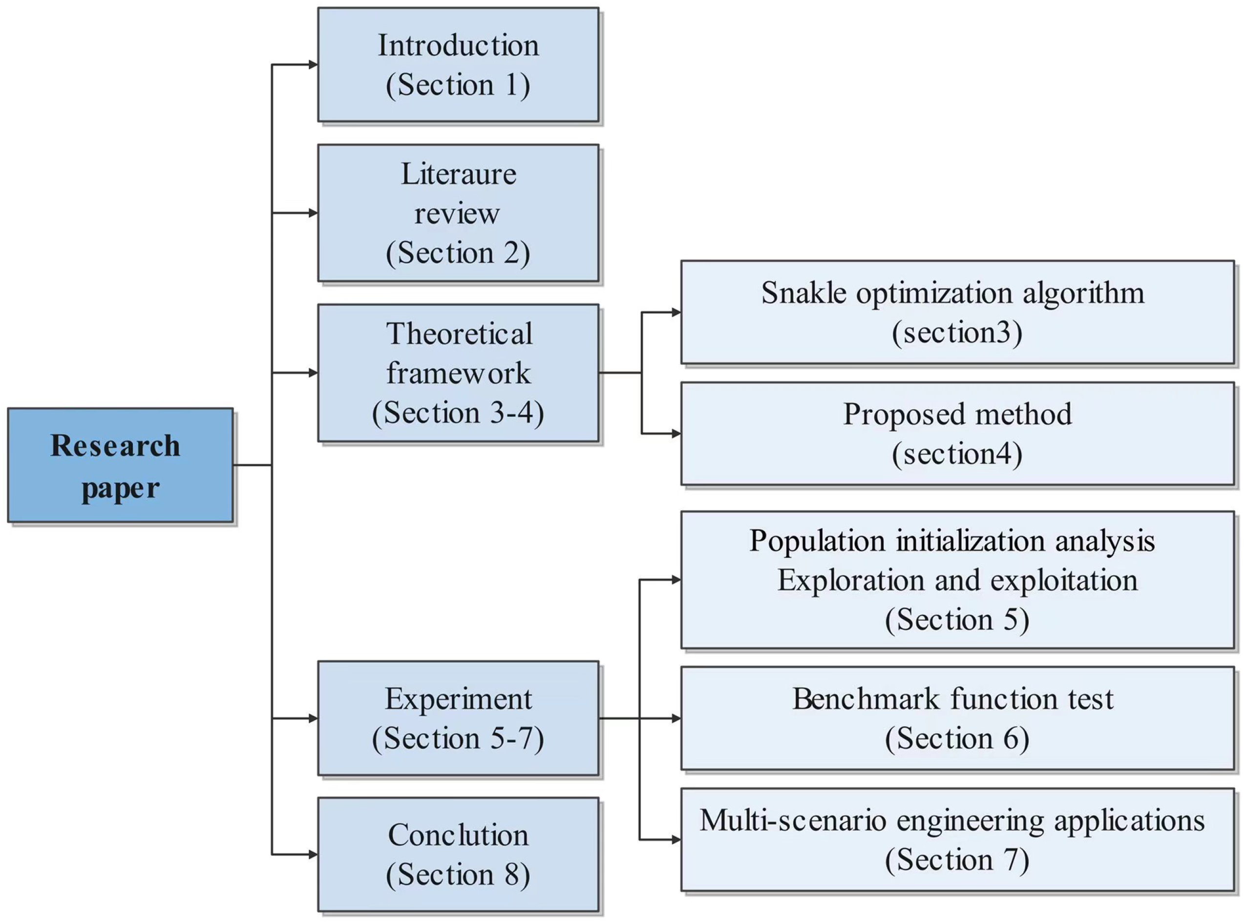
Figure 1.
Enter Caption
2. Literature Review
Metaheuristic algorithms primarily encompass Evolutionary Algorithms (EA)[8], Physics-inspired Algorithms (PhA)[9], Human Behavior-Based Algorithms(HBA)[10], and Swarm Intelligence algorithms (SIA)[11].
EA are optimization techniques grounded in the principles of natural selection and genetics. The fundamental concept is to emulate the evolutionary process of organisms through mechanisms such as selection, crossover, and mutation, thereby continually enhancing the quality of solutions. Genetic Algorithms (GA) [12] represent a category of optimization algorithms derived from natural selection and genetic principles, utilized to address complex optimization challenges. Genetic Programming is a methodology for the automatic generation and selection of computer programs, inspired by the process of biological evolution, to fulfill user-specific tasks. Differential Evolution Algorithms (DEA)[13] attain optimal solutions by discarding subpar individuals and preserving superior ones.Cultural Algorithms (CA)[14] employ an additional domain termed the "belief space" to aggregate and exploit pertinent information about the behavior of individuals within the search space. Since their inception, Cultural Algorithms have been effectively extended and applied to resolve a variety of problems across different technological fields.
PHA draw inspiration from physical phenomena such as gravity, electromagnetism, and quantum mechanics. These algorithms emulate physical processes to determine ideal resolutions to intricate issues. Simulated Annealing (SA)[15] is modeled after the metallurgical technique of heating a material to its liquefaction point and then incrementally cooling it to create a highly structured solid form. By gradually lowering the system’s "temperature," SA strives to identify the global optimal solution for the problem. Particle Swarm Optimization (PSO)[16] aims to achieve the optimal resolution by replicating the behavior of particles within the search space. In this method, each particle symbolizes a possible solution and continuously refines and enhances its position by learning from the collective experiences of the swarm. Quantum-inspired Evolutionary Algorithms (QIEA)[17] draw from the advancements in quantum mechanics, employing concepts such as quantum bits and superposition states for optimization computations. This algorithm seeks the optimal solution through the progression of quantum states, thereby decreasing the time required for large-scale data processing and enhancing efficiency.
HBBA focus on improving solution quality by mimicking human learning and decision-making processes. These algorithms optimize by emulating human expert behaviors, decision tree structures, reinforcement learning, and case-based reasoning. The Case-Based Reasoning Algorithm (CBRA)[18] addresses current problems by recalling and applying successful past cases. This algorithm emulates the human problem-solving approach through experience and is utilized in fields like medical diagnosis, legal judgment, and fault diagnosis.The Reinforcement Learning Algorithm (RLA)[19] learns optimal strategies through interaction with the environment. Using reward and punishment mechanisms to mimic human trial-and-error learning, reinforcement learning algorithms continuously optimize behavior strategies and are widely applied in AI, robot control, and financial trading.
SIA are approaches designed to tackle complex optimization challenges by mimicking the collective behavior found in nature. Drawing inspiration from the activities of biological groups such as ants, bees, birds, and fish, these algorithms leverage simple interactions among individual agents to produce sophisticated and intelligent collective behaviors. Ant Colony Optimization (ACO)[20] is modeled after the foraging patterns of ants. It seeks optimal solutions, particularly in path optimization tasks, by replicating the movements of virtual ants within the search space and updating pheromone trails. The Salp Swarm Algorithm (SSA)[21] draws its conceptual framework from the swarming behavior of salp chains. SSA has proven to be highly effective in optimizing various engineering design problems.
Since the invention of the SO[22],numerous researchers have enhanced this algorithm and developed various improved versions for engineering applications. Karam Khairullah Mohammed and colleagues optimized the SO for fast and precise maximum power tracking in photovoltaic systems. Chaohua Yan and Navid Razmjooy crafted an advanced version of the Snake Optimization Algorithm and applied it with Convolutional Neural Networks for nodule prediction on the âIQ-OTH/NCCD-Lung Cancer Dataset.t[23]. Weimin Zheng and his team introduced a compact strategy in the Snake Optimization algorithm for population probability modeling, improving indoor positioning accuracy[24] . Yang Rui and colleagues proposed an efficient enhanced Snake Optimizer ,and benchmarked its performance against several algorithms in terms of benchmark functions and engineering design applications[25]. Building on the steps of the Snake Optimization Algorithm and previous improvement strategies, this paper innovatively integrates three algorithms into the original Snake Optimization Algorithm. The improved algorithm is applied to 4 engineering questions, and comparative experiments have been conducted to evaluate its performance.
3. Snake Optimization Algorithm
3.1. Initialization
The original Snake optimization begins by generating a random population with a uniform distribution to initiate the optimization process. The initial population can be determined using the following equation:
In this context, denotes the position of the i-th individual, r is a randomly generated number within the range [0, 1], and and represent the minimum and maximum bounds of the problem, respectively.
3.2. Dividing the Swarm into Two Equal Groups: Males and Females
SO will set up a simplified gender distribution scenario. Assuming a balanced population composition consisting of 50% males and 50% females. To analyze this binary structure, we further divided the population into two distinct groups: the male group and the female group. It is worth noting that this classification mechanism is similar to the organizational structure of bee colonies in nature. Although there are significant differences in essence, in this context, we adopted an analogy approach to specifically define and distinguish these two gender groups through formulas (2) and (3) for subsequent data processing and analysis.
Where N, , are the total number of individuals, the number of males, and the number of females, respectively.
3.3. Evaluate Each Group and Define Temperature and Food Quantity
In order to optimize the selection process, we identified the best performing males from the male group, labeled as , while selecting the best performing females from the female group, labeled as . In addition, we also focused on the importance of food location as one of the key factors affecting survival and reproduction.
- Temperature () can be expressed as:
- The definition of quantity (Q) is:
3.4. Exploration Phase (No Food)
If (Threshold = 0.25), the snakes search for food by selecting random positions and updating their positions accordingly. To model the exploration phase, the following equation is used:
Here, denotes the position of the male, indicates the position of a randomly selected male, is a random number between 0 and 1, and represents the male’s ability to find food, calculated as follows:
In this description, represents the fitness value of a randomly selected male individual , while specifically refers to the fitness value of the i-th individual in the male population. To evaluate the performance of randomly selected individuals relative to other individuals in their group (i.e., male group), we introduced a comparison mechanism. Among them, is set as a preset constant with a value of 0.05, which plays a regulatory role in the comparison process and may be used to control the selection pressure or adjust the sensitivity of fitness evaluation.
We defined as specific location identifiers for each member in the female population. For random selection or comparison, we introduce which represents the position of a female individual selected through a random process involving a random number between 0 and 1. In addition, the ability of female populations to search for food is quantified by the parameter , which has been calculated based on specific attributes or behaviors of female individuals:
We defined is the fitness of , and is the fitness of the ith individual in the female group.
3.5. Exploitation Phase (Food Exists)
If :
- If the temperature (0.6) (hot):
The snakes will move to the food only:
Where represents the position of the individual (male or female), is the position of the best individuals, and is a constant equal to 2.
- If the temperature (0.6) (cold):
The snake will be in either fight mode or mating mode.
- Fight Mode:
- Mating Mode:
3.6. Termination Conditions
The algorithm continues until the termination conditions are met. This could be a set number of iterations, a convergence criterion.
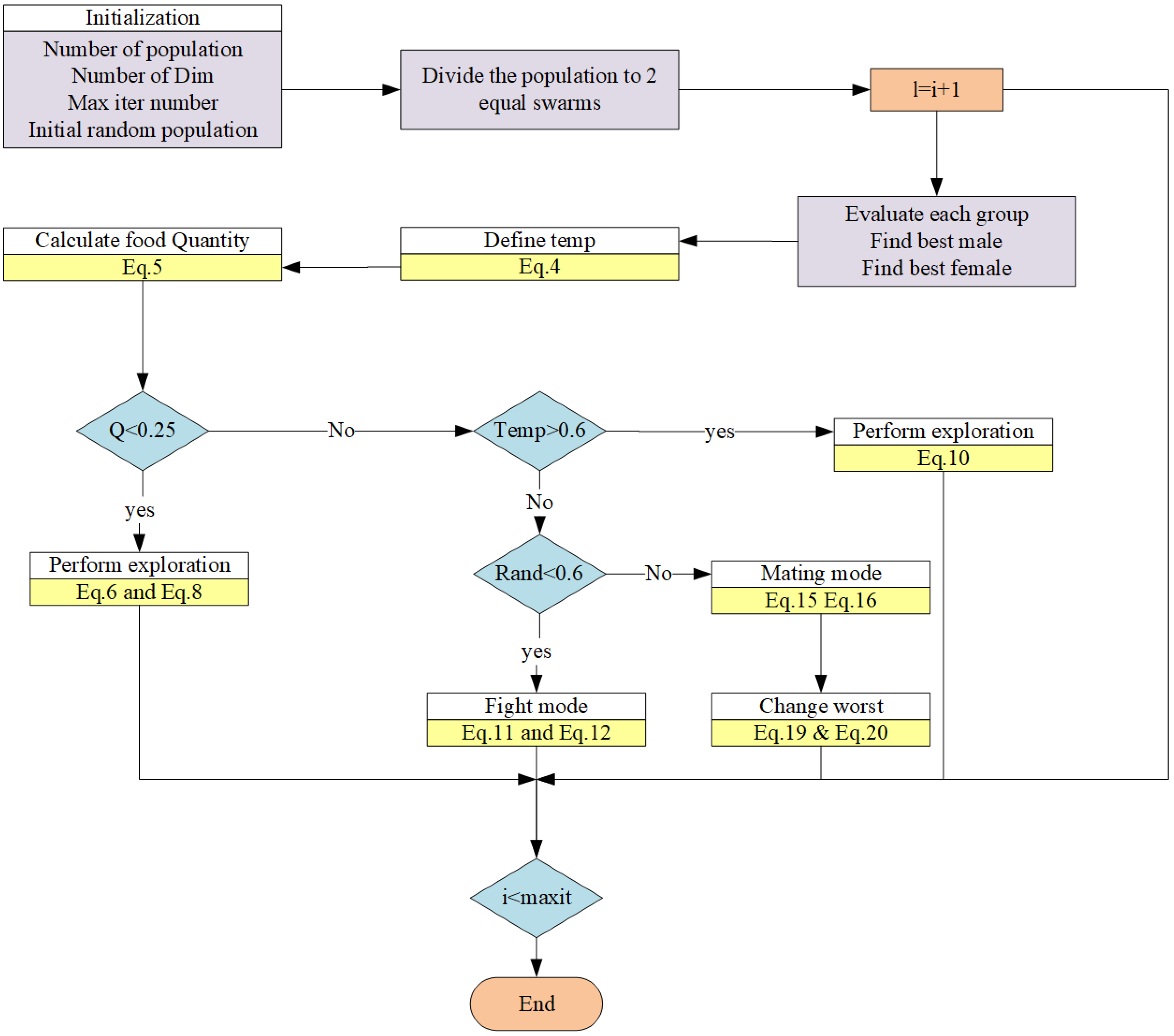
3.7. Algorithm Flowchart
4. Proposed Method
4.1. Initialization Using Sobol Sequences
During the initial phase of the Snake Optimization (SO) framework, the initialization stage is critical for setting the foundation for the subsequent exploration and exploitation phases[26,27]. Conventional random initialization techniques may lead to an imbalanced exploration of the search space. This imbalance can reduce the probability of identifying the global optimal solution, especially during the early stages of iteration. To address the uneven coverage and enhance the algorithm’s comprehensive search ability throughout the entire search space, we employ Sobol sequences in place of random initialization. Sobol Sequences[28] are low-discrepancy sequences that help generate points more evenly distributed in high-dimensional space. Compared to initial populations generated using non-structured random methods, points generated using Sobol sequences are distributed more uniformly throughout the entire unit hypercube. This characteristic ensures comprehensive coverage of the search space, particularly advantageous during the initialization phase. In ISO, the process of initializing the data using Sobol sequences is as follows:
- Generate a Sobol sequence , where and d is the dimensionality of the problem.
- Map the generated points to the search space defined by the lower and upper bounds, and respectively.
- Assign the mapped points to the initial positions of the individuals in the swarm.
The position of each individual in the swarm is computed using the following equation:
Where ⊙ denotes the element-wise multiplication.
Using Sobol sequences for initialization allows for the even dispersion of the initial population throughout the search space, enabling broad coverage. This sets a solid foundation for subsequent optimization stages, providing a favorable starting point.
4.2. Incorporating the RIME Optimization Algorithm
RIME[29] is an efficient optimization algorithm based on the physical phenomenon of rime-ice. The RIME algorithm simulates the growth processes of soft-rime and hard-rime, constructing a soft-rime search strategy and a hard-rime puncture mechanism. Integrating this strategy within the ISO framework can enhance the exploration and exploitation behaviors in optimization methods, thereby improving the convergence capability of ISO. The computational method is as follows.
Where
And
The integration of the RIME algorithm into the original snake optimization framework is critical[30], necessitating a rigorous analysis of the effects on the convergence behavior and exploratory characteristics of the algorithm. The newly proposed equations (22), (23), and (24) introduce a refined mechanism for updating the position vectors.This strategy successfully balances the need for thorough exploration of the global search space with the requirement for intensive exploitation of local regions, achieved through the modulation of search amplitude by the temperature-based factor and the adaptive scaling factor , both of which are influenced by the iteration count t and the problem’s dimensional size W.
4.3. Lens Imaging Reverse Learning
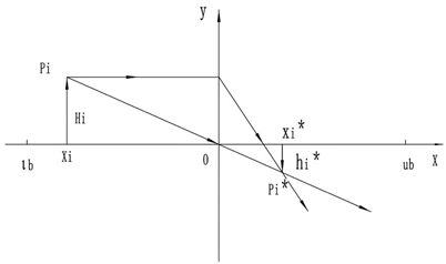
The population distributed in the function space can lead the group to find good resources due to its wide search range and flexible search methods[31]. Once some populations fall into local optima, the overall performance of the algorithm declines. Therefore, enhancing the search range of the finders is particularly important. General learning strategies have achieved good results in some optimization algorithms, but they have little impact on the algorithm’s performance. This is because general learning strategies can only perform reverse solving in local spaces, which, while enriching the population’s diversity, still have a narrow search range and lose the ability to explore the global space. [32]To improve the population’s search capability, an inverse learning strategy based on lens imaging is proposed and applied to the position update formulas of all individuals in the population to enhance the global search capability of ISO. is the search space for solutions, and y represents the function value. Suppose there is a system with a height of , and its projection at point x is x; this system is reproduced as another system on the other side with a lens focal length that is halved midway, with a height of and a projection at point as . According to the principle of lens imaging, we obtain[33]:
Let ; then Equation (9) can be rewritten as:
Equation (26) is the transformation formula for the back focal length of the original lens on the halved side.
The scaling factor k is a freely selectable parameter that can be dynamically adjusted according to different problems. In this paper, the selection of the k value is based on the results of multiple experiments, which can maximize the solving ability of the ISO algorithm[33].
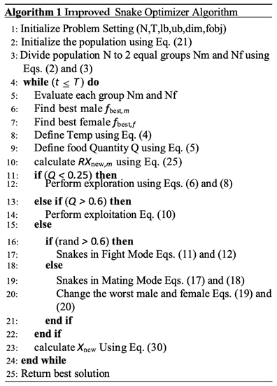
The pseudocode is as follows:
5. Population Initialization and Exploration-Exploitation Analysis
In most cases, employing a strategy for uniform population initialization allows the initial population[34,35] to be distributed across every corner of the space, providing a solid foundation for algorithm iterations. During the algorithm’s iteration process, the balance between exploration and exploitation[36,37] is also a factor worth examining. Section 5.1 and Section 5.2 provide a detailed explanation of the analysis process.
5.1. Population Initialization Analysis
The following figure shows the initialization state of the ISO population, and the table below presents the statistical results measured using three algorithms: Star Discrepancy, Average Nearest Neighbor Distance, and Sum of Squared Deviations (SSD).
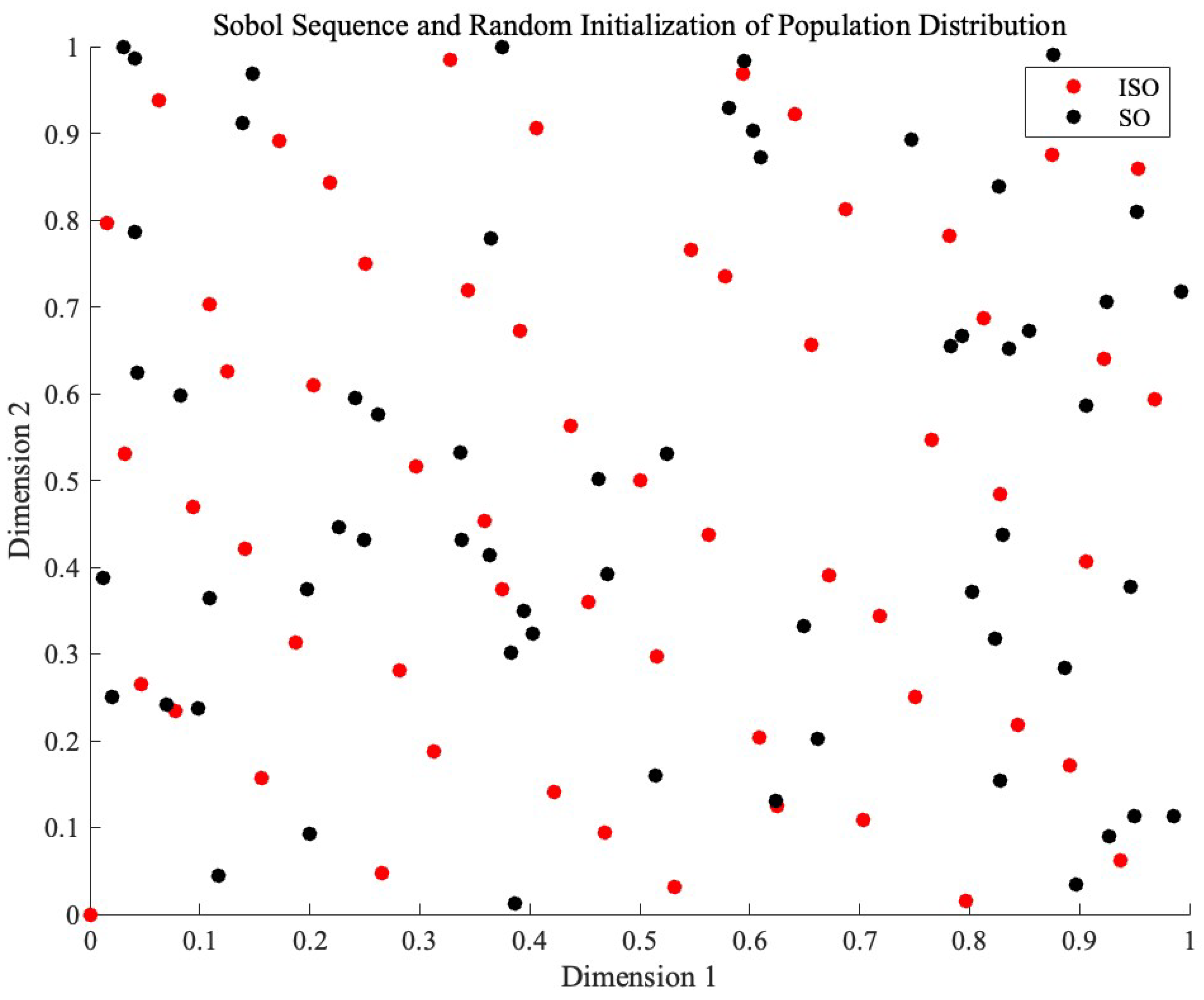
Figure 3.
The picture of the comparison between ISO with Sobol initialization and SO with random initialization.
Figure 3.
The picture of the comparison between ISO with Sobol initialization and SO with random initialization.

Table 1.
Precision Data
| Parameter | SO (Random Initialization) | ISO (Sobol Sequence) |
|---|---|---|
| Star Discrepancy | 0.133966 | 0.047965 |
| Average Nearest Neighbor Distance | 0.069264 | 0.086739 |
| Sum of Squared Deviations (SSD) | 11.255603 | 9.990234 |
The three metricsâStar Discrepancy,Average Nearest Neighbor Distance and Sum of Squared Deviations (SSD) are crucial for evaluating the uniformity of population distributions. The specific calculations are as follows.
Star Discrepancy
Description: The star discrepancy measures the overall spatial uniformity of a point set within a unit cube. By calculating the maximum difference between the number of points within subrectangles and the expected number of points in a perfectly uniform distribution, the uniformity can be assessed. A smaller star discrepancy indicates a more uniform distribution, while a larger star discrepancy indicates less uniformity.[38]
Formula:
where n is the total number of points, d is the dimension, is a point in the set, is a reference point, is the coordinate of point in the kdimension.
Average Nearest Neighbor Distance
Description: The average nearest neighbor distance measures the uniformity of point distributions in space. By calculating the distance from each point to its nearest neighbor and taking the average of these distances, one can determine the distribution pattern. A larger average nearest neighbor distance indicates a more uniform distribution, while a smaller distance indicates clustering.[39] Formula:
where n is the total number of points, and are points in the set, and denotes the Euclidean distance between point and point .
Sum of Squared Deviations (SSD)
Description: The sum of squared deviations evaluates the dispersion of a set of points relative to a central location. By calculating the squared distance from each point to the center and summing these values, one can quantify the spread of the point set. A smaller SSD indicates a more uniform distribution, while a larger SSD indicates greater dispersion.[40] Formula:
where n is the total number of points, d is the dimension, is the coordinate of the i-th point in the j-th dimension, and is the coordinate of the central point in the j-th dimension.
The Sobol sequence initialization (ISO) demonstrates superior uniformity compared to random initialization (SO). Specifically, the ISO exhibits a higher Average Nearest Neighbor Distance (0.086739 compared to 0.069264). Moreover, the ISO shows a lower SSD (9.990234 compared to 11.255603) and a significantly lower Star Discrepancy (0.047965 compared to 0.133966). These results collectively affirm that ISO provides a more homogeneous initial population than SO, making it a preferable choice for applications requiring highly uniform distributions.
5.2. Exploration-Exploitation Analysis
The key to constructing effective metaheuristic algorithms is how to find a reasonable balance between the two. Excessive search can trap the algorithm in a large number of solution sets and prevent it from converging quickly; Moreover, excessive development can lead to algorithms easily falling into local optima, thereby losing the global optimum. So, the most ideal algorithm should be able to deeply mine it based on the search process and the quality feedback of the current solution, while ensuring the ability to search on a large scale, to achieve efficient and robust optimization effects. This dynamic strategy not only improves the algorithm’s adaptability, but also enhances its robustness, ensuring satisfactory optimization results in various situations
In the context of metaheuristic algorithms, exploration and exploitation are considered two fundamental components[42]. Exploration involves investigating new solutions within the solution space, with the goal of discovering superior solutions in unexplored areas. Conversely, exploitation focuses on established solution spaces, performing searches within the local vicinities of known solutions to identify potentially better outcomes. Achieving a well-balanced combination of exploration and exploitation not only enables the algorithm to converge swiftly to optimal solutions, thereby improving search efficiency, but also provides the versatility to address a wide range of optimization challenges and complexities, demonstrating remarkable adaptability and robustness. An effective algorithm must maintain an optimal balance between these two aspects.Div(t) is a measure of dimension diversity calculated by Eq. (33). Here, represents the position of the dimension, and denotes the maximum diversity throughout the entire iteration process.
Figure 4 intuitively illustrates the balance between exploration and exploitation in ISO using the 30-dimensional CEC-2017 test functions. From the graph, it is evident that the intersection point of the exploration and exploitation ratio in the ISO algorithm.During the initial phase, a comprehensive exploration of the global search space is conducted, gradually transitioning to a local exploitation phase. Notably, in the later iterations of all functions, ISO maintains a relatively high level of exploitation, contributing to an improved convergence rate and search accuracy. Throughout the entire iterative process, ISO preserves a dynamic balance between exploration and exploitation. Consequently, ISO exhibits significant advantages in avoiding local optima and premature convergence.
6. Benchmark Function Test
The hardware configuration used in this experiment includes an Intel i9-13900K CPU, 64GB of memory, and a 4070 GPU. The software configuration consists of the Windows 10 operating system and MATLAB 2023a.To validate the performance of the ISO algorithm, we compared it with highly-cited and state-of-the-art algorithms.We selected SO, RIME, SCA[43], WOA[44], and GWO[45] as the competing algorithms.Among these, SO and RIME, proposed in 2020 and 2023 respectively, are considered the latest algorithms. SCA, WOA, and GWO, which have been cited 4,524 times, 11,027 times, and 15,545 times respectively, are considered highly cited algorithms. We selected 23 standard test functions. They are specifically designed to address significant challenges in optimization, becoming the gold standard for performance comparison in the field of metaheuristic algorithms, as shown in Picture 2[46]. Functions Fl to F7 are uni-modal functions with a single global optimum, utilized to evaluate the algorithm’s developmental capabilities. Functions F8 to F13 are multimodal functions with one global optimum and several local optima, enabling the testing of the algorithm’s global search capabilities. Functions F14 to F23 are multimodal functions with fixed dimensions, suitable for simultaneously testing the algorithm’s developmental and search capabilities.
6.1. Convergence Behavior Analysis
In this section, we focus on analyzing the convergence behavior of different algorithms. For each set of results, the left figure presents the 3D image of the test function, vividly illustrating the complexity of the problem, while the right figure shows the convergence curves of different algorithms when solving various problems. All algorithms were configured with a population size of N=40 and a maximum of T=500 iterations.
he convergence curve results indicate that the ISO algorithm achieves rapid convergence and lower function values in most cases. Specifically, ISO performs similarly to other competitive algorithms on functions F8, F15, F16, F19, and F20, while achieving lower function results with fewer iterations on the remaining 18 test functions. Notably, ISO demonstrates superior performance on functions F1, F2, F3, F4, F7, and F10 compared to competitive algorithms. This underscores ISOâs superior convergence speed and its enhanced capability to explore global optimal solutions compared to SO and other competitive algorithms.
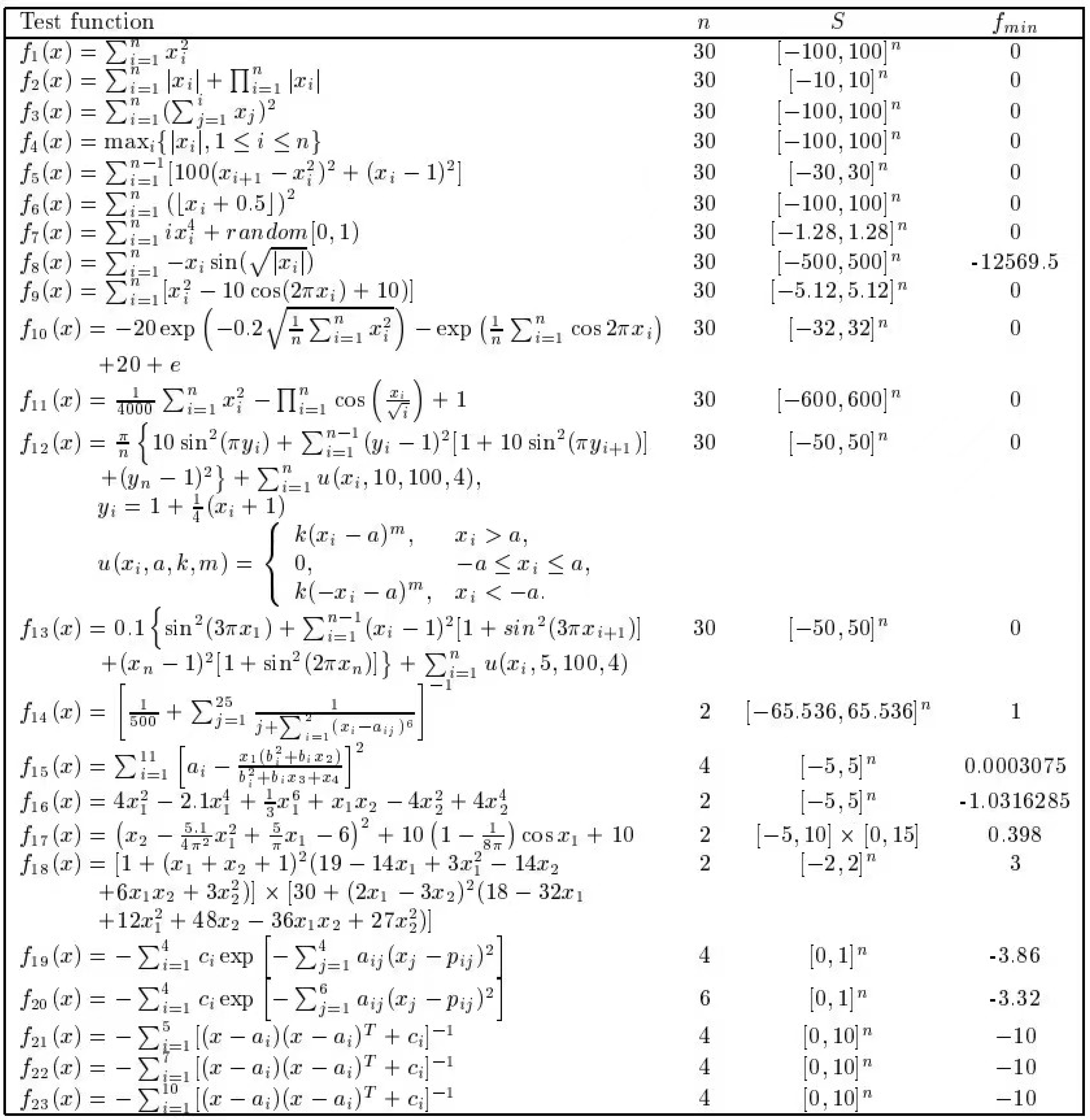
Figure 5.
23 Test Function
6.2. Detailed Analysis of the Benchmark Function
To comprehensively demonstrate the effectiveness of ISO, the maximum value, standard deviations, averages, medians, and minimum values obtained by six algorithms when solving 23 different functions were meticulously recorded. Boxplots were plotted based on the experimental results [47], and Wilcoxon rank-sum tests were conducted [48].In Wilcoxon rank-sum tests, a significance threshold of 5% was established. If the computed value falls below 5%, it denotes a statistically significant distinction between the two algorithms; if the computed value surpasses 5%, it signifies no statistically significant difference. NaN values indicate that the performance of the two algorithms is similar and cannot be compared.
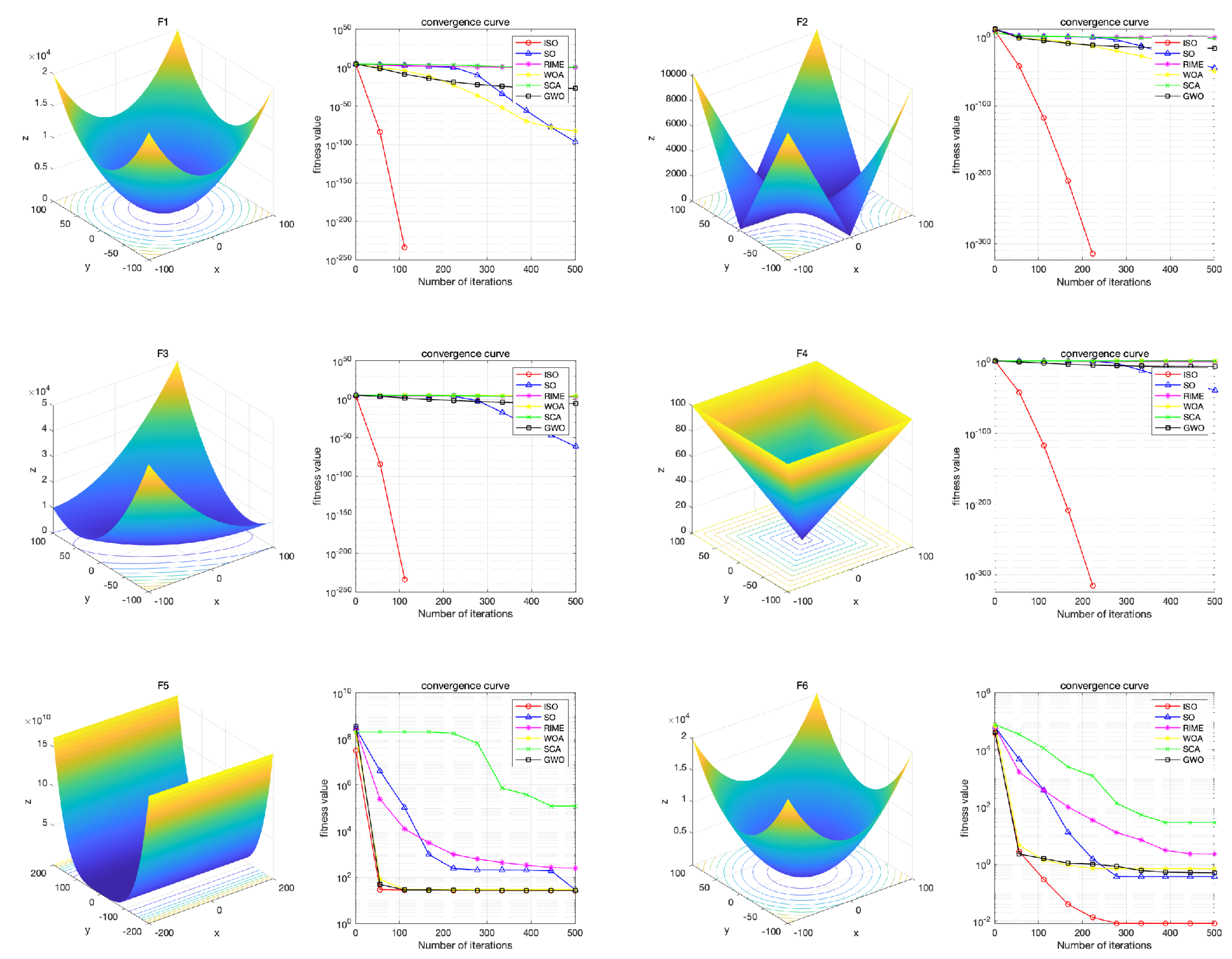
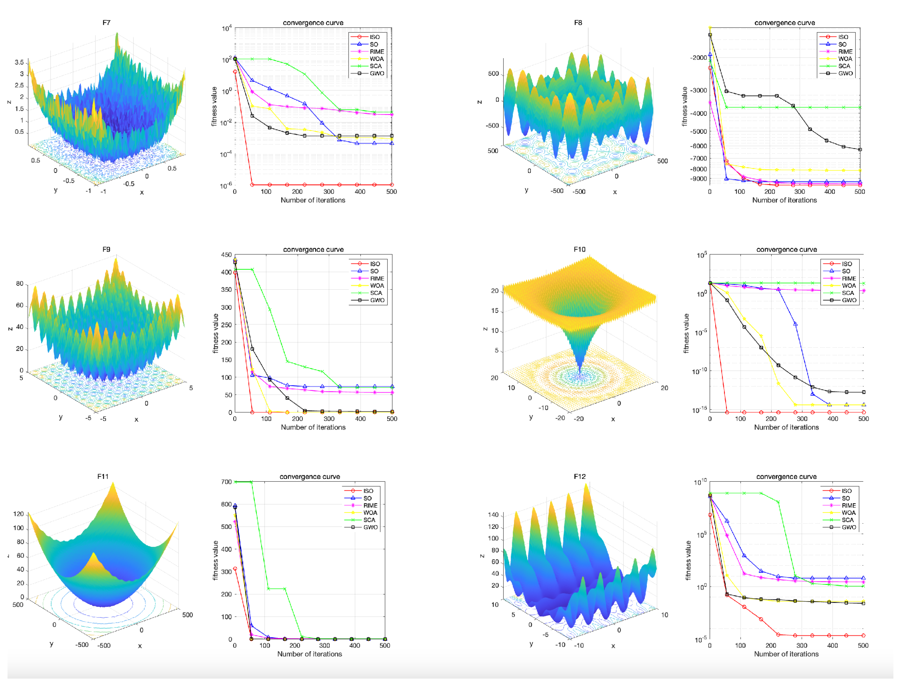
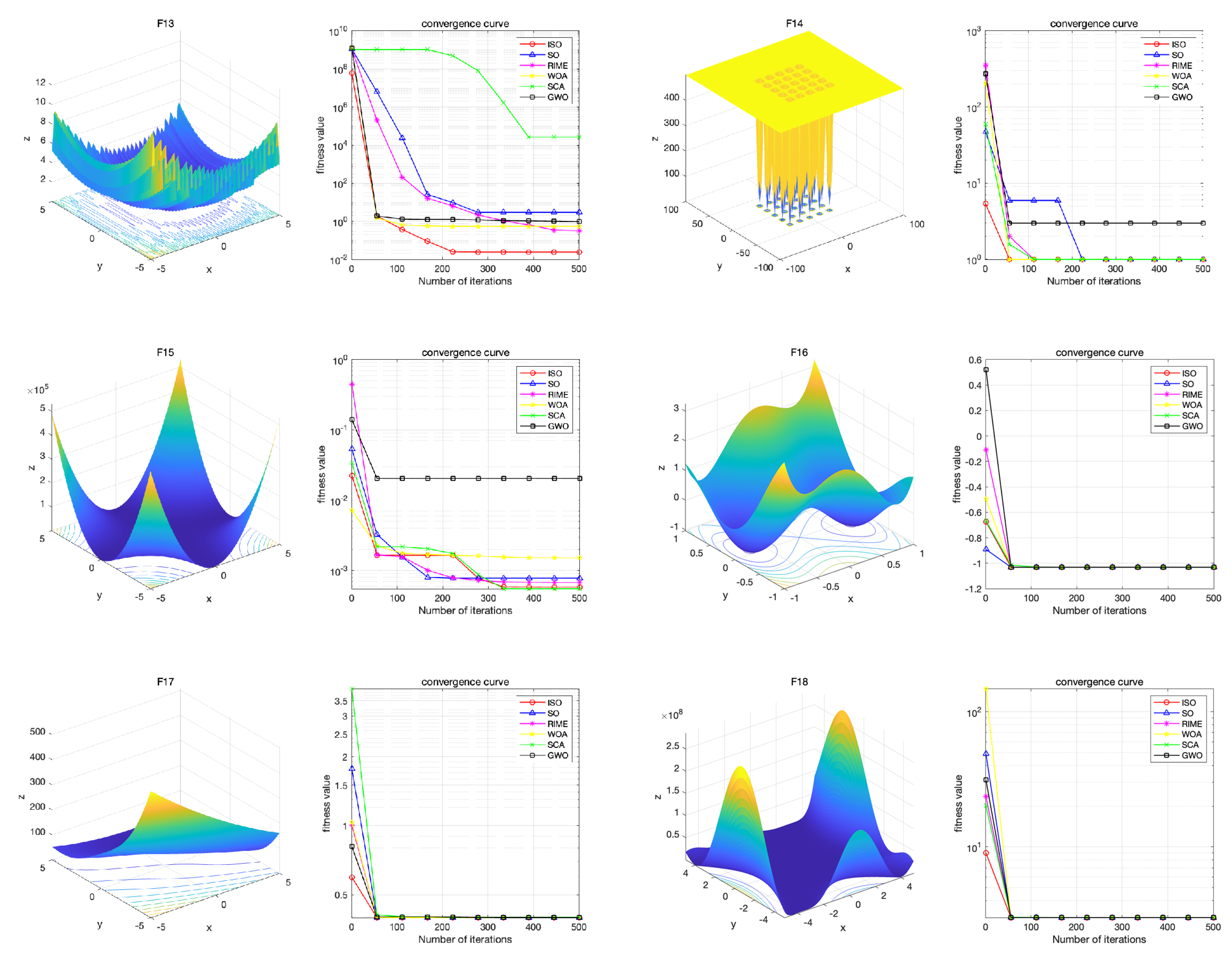
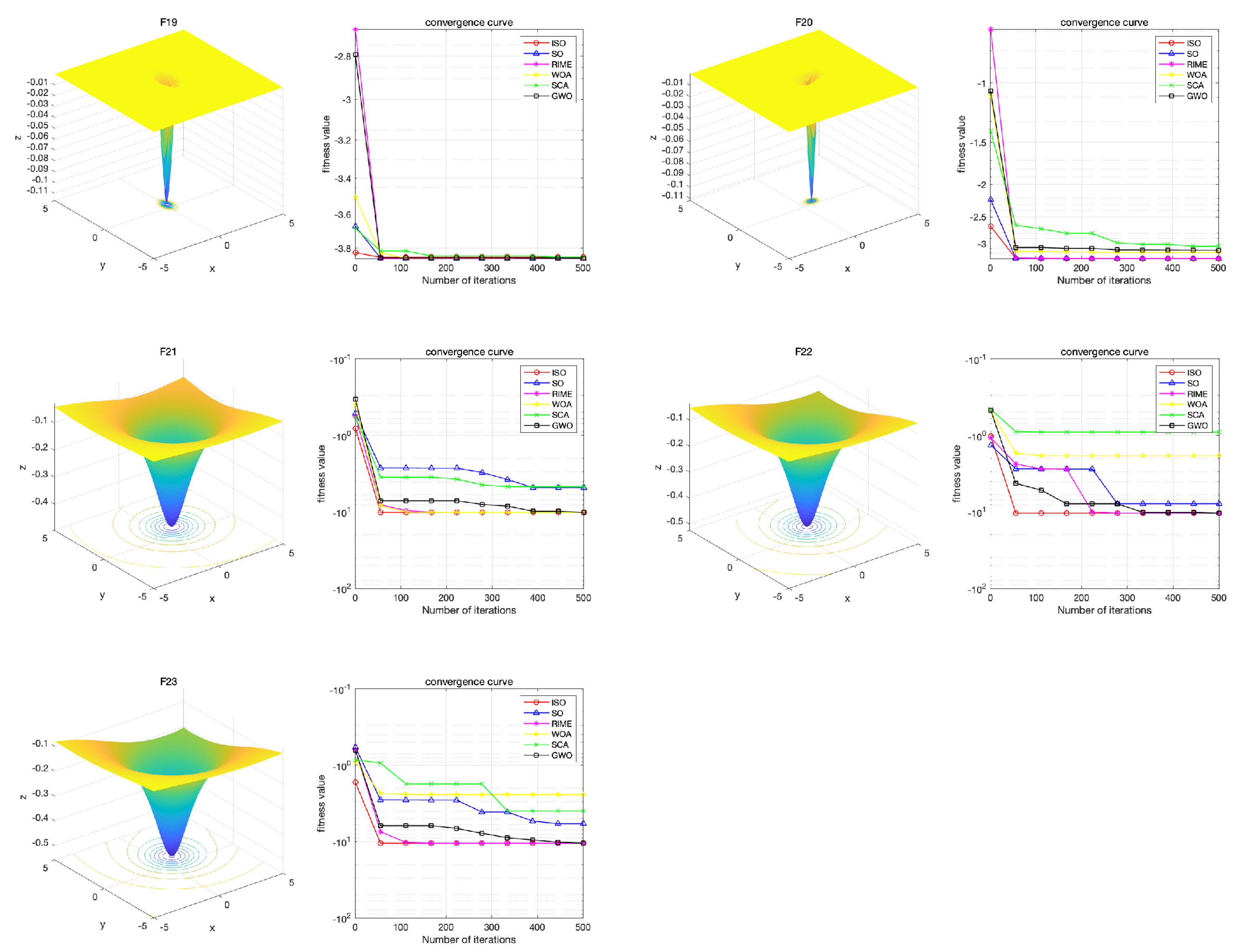
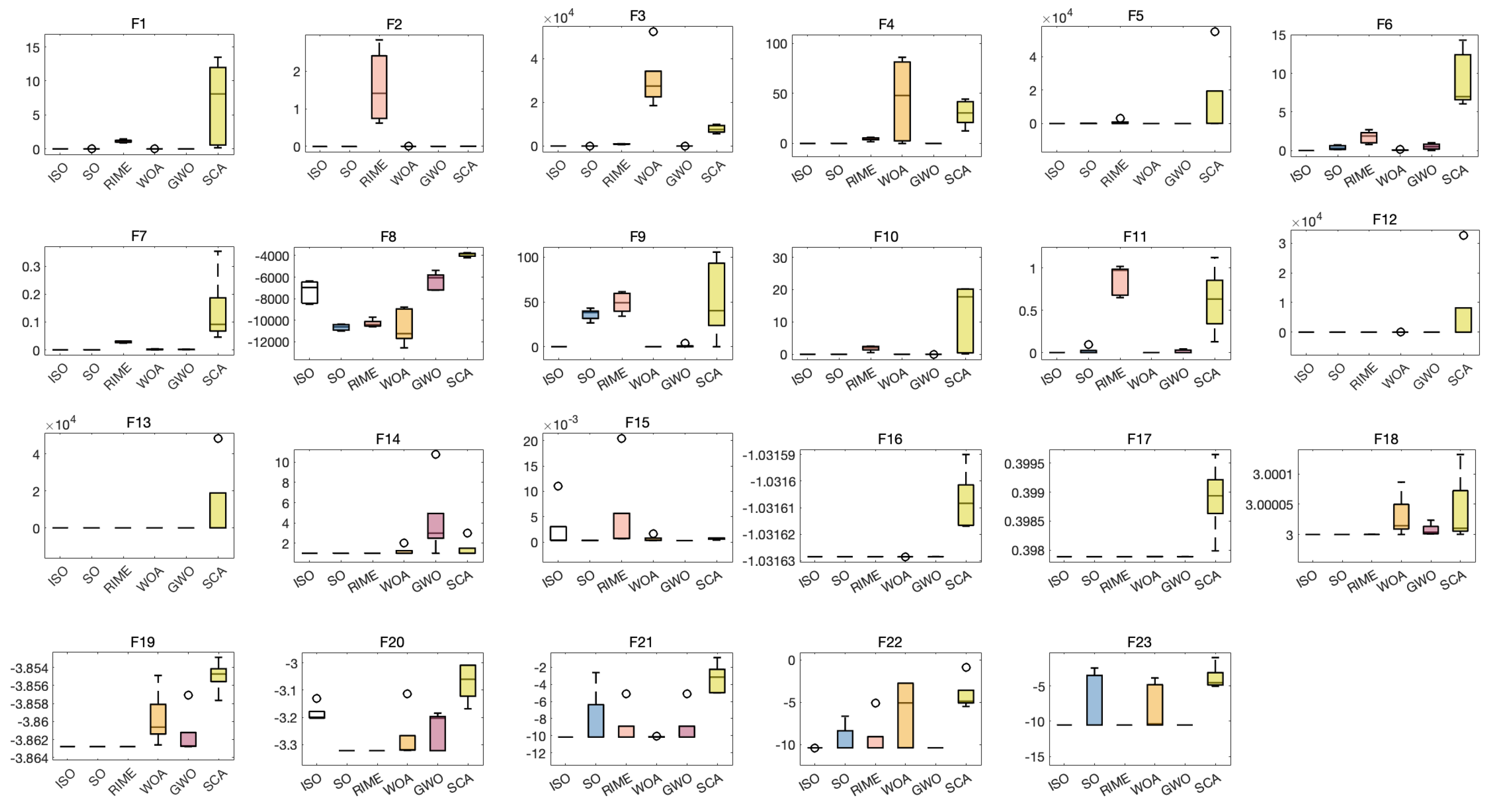
Figure 6.
Test Function F1-F6
Figure 7.
Test Function F7-F12
Figure 8.
Test function F13-F18
Figure 9.
Test Function F19-F23
Figure 10.
Result of Boxplot (maximum value,Standard Deviation,Average Value,Median Value,Minimum Value)
Figure 10.
Result of Boxplot (maximum value,Standard Deviation,Average Value,Median Value,Minimum Value)
Table 2.
Precision Data
| ISO | SO | RIME | WOA | GWO | SCA | |
|---|---|---|---|---|---|---|
| F1 Maximum value | 0 | 1.6156e-101 | 0.79632 | 6.2667e-90 | 2.9418e-32 | 0.018227 |
| F1 Standard Deviation | 0 | 3.0829e-96 | 0.82593 | 3.6085e-80 | 2.1056e-30 | 5.8823 |
| F1 Average Value | 0 | 2.1112e-96 | 1.6654 | 1.1703e-80 | 1.3072e-30 | 3.4484 |
| F1 Median Value | 0 | 5.977e-97 | 1.5769 | 6.7968e-86 | 3.3005e-31 | 0.38834 |
| F1 Minimum Value | 0 | 8.8973e-96 | 3.7043 | 1.1438e-79 | 5.9552e-30 | 15.6586 |
| F2 Maximum value | 0 | 1.5847e-46 | 0.53371 | 2.392e-57 | 2.0754e-19 | 4.9074e-05 |
| F2 Standard Deviation | 0 | 5.2612e-44 | 0.4858 | 1.0992e-52 | 6.9339e-19 | 0.0088126 |
| F2 Average Value | 0 | 3.0919e-44 | 0.90418 | 4.0029e-53 | 1.1986e-18 | 0.0077208 |
| F2 Median Value | 0 | 6.2431e-45 | 0.75306 | 2.2097e-55 | 9.5475e-19 | 0.0039093 |
| F2 Minimum Value | 0 | 1.7346e-43 | 2.0696 | 3.5024e-52 | 2.2958e-18 | 0.027479 |
| F3 Maximum value | 0 | 1.1664e-67 | 384.3923 | 19995.9104 | 1.1741e-09 | 1525.2676 |
| F3 Standard Deviation | 0 | 1.1251e-59 | 304.3303 | 8915.4857 | 6.7043e-07 | 4607.7335 |
| F3 Average Value | 0 | 5.4436e-60 | 854.9073 | 35898.743 | 4.7077e-07 | 10138.0775 |
| F3 Median Value | 0 | 4.0227e-63 | 827.1762 | 36953.5381 | 8.146e-08 | 11024.7254 |
| F3 Minimum Value | 0 | 3.1096e-59 | 1402.0287 | 48574.3146 | 1.5437e-06 | 16323.6006 |
| F4 Maximum value | 0 | 5.1604e-43 | 3.4574 | 3.6318 | 9.928e-09 | 9.027 |
| F4 Standard Deviation | 0 | 2.964e-41 | 1.6497 | 30.5907 | 1.2116e-07 | 6.7815 |
| F4 Average Value | 0 | 2.3189e-41 | 6.0868 | 41.9403 | 1.5419e-07 | 21.0788 |
| F4 Median Value | 0 | 7.0935e-42 | 5.6659 | 37.7864 | 1.2797e-07 | 22.0562 |
| F4 Minimum Value | 0 | 8.5465e-41 | 9.573 | 85.1509 | 3.9006e-07 | 29.6541 |
| F5 Maximum value | 24.7598 | 28.8231 | 52.2265 | 27.2556 | 26.179 | 82.5777 |
| F5 Standard Deviation | 0.59228 | 54.4177 | 458.7257 | 0.21881 | 0.67703 | 18885.0142 |
| F5 Average Value | 25.3956 | 54.7162 | 445.2294 | 27.67 | 27.1109 | 9078.5037 |
| F5 Median Value | 25.1402 | 28.9162 | 353.4091 | 27.7765 | 27.1375 | 2236.0169 |
| F5 Minimum Value | 26.4062 | 159.0777 | 1680.5587 | 27.866 | 27.9309 | 61772.1619 |
| F6 Maximum value | 0.00022812 | 0.12251 | 0.43999 | 0.028669 | 0.24964 | 5.1908 |
| F6 Standard Deviation | 0.0021647 | 0.23817 | 0.80692 | 0.058841 | 0.25713 | 11.0357 |
| F6 Average Value | 0.0021236 | 0.36652 | 1.5199 | 0.11855 | 0.54914 | 12.1774 |
| F6 Median Value | 0.0013819 | 0.29371 | 1.5159 | 0.11984 | 0.50366 | 7.2204 |
| F6 Minimum Value | 0.0072755 | 0.90824 | 3.017 | 0.22648 | 0.99279 | 35.4493 |
| F7 Maximum value | 5.9325e-06 | 9.8841e-05 | 0.0066106 | 7.2842e-05 | 0.00054522 | 0.013495 |
| F7 Standard Deviation | 1.8724e-05 | 0.00013572 | 0.013488 | 0.0037777 | 0.0013254 | 0.064203 |
| F7 Average Value | 3.4074e-05 | 0.00027541 | 0.030573 | 0.0027863 | 0.001424 | 0.066626 |
| F7 Median Value | 3.7737e-05 | 0.000272 | 0.030255 | 0.0014118 | 0.0010548 | 0.042689 |
| F7 Minimum Value | 6.2134e-05 | 0.00053759 | 0.047252 | 0.012901 | 0.0049689 | 0.21389 |
| F8 Maximum value | -8941.9029 | -11202.8618 | -11212.2637 | -12567.4537 | -7241.0015 | -3964.0364 |
| F8 Standard Deviation | 705.6836 | 419.4716 | 352.7549 | 1680.0918 | 470.9275 | 158.2354 |
| F8 Average Value | -7979.4087 | -10433.1947 | -10551.4162 | -10362.0449 | -6462.9317 | -3734.5521 |
| F8 Median Value | -7675.3417 | -10305.079 | -10469.8854 | -9965.6122 | -6406.543 | -3705.014 |
| F8 Minimum Value | -7314.8199 | -10014.2347 | -10071.167 | -8522.1804 | -5790.5202 | -3541.7477 |
| F9 Maximum value | 0 | 32.1315 | 35.0709 | 0 | 0 | 0.16486 |
| F9 Standard Deviation | 0 | 9.6948 | 16.224 | 0 | 1.895 | 38.8566 |
| F9 Average Value | 0 | 47.3503 | 58.4451 | 0 | 1.087 | 46.9693 |
| F9 Median Value | 0 | 47.4626 | 55.8667 | 0 | 1.7053e-13 | 52.2689 |
| F9 Minimum Value | 0 | 64.4491 | 88.9517 | 0 | 5.2149 | 99.3974 |
| F10 Maximum value | 4.4409e-16 | 4.4409e-16 | 1.5369 | 4.4409e-16 | 5.0182e-14 | 0.047233 |
| F10 Standard Deviation | 0 | 1.1235e-15 | 0.36392 | 2.4841e-15 | 7.1937e-15 | 10.1462 |
| F10 Average Value | 4.4409e-16 | 3.6415e-15 | 2.0332 | 5.4179e-15 | 5.7643e-14 | 10.2912 |
| F10 Median Value | 4.4409e-16 | 3.9968e-15 | 2.0954 | 5.7732e-15 | 5.7288e-14 | 10.3939 |
| F10 Minimum Value | 4.4409e-16 | 3.9968e-15 | 2.6224 | 7.5495e-15 | 6.7946e-14 | 20.352 |
| F11 Maximum value | 0 | 0 | 0.70668 | 0 | 0 | 0.32025 |
| F11 Standard Deviation | 0 | 0.19571 | 0.1102 | 0 | 0.0072452 | 0.27456 |
| F11 Average Value | 0 | 0.12263 | 0.87297 | 0 | 0.0044876 | 0.81096 |
| F11 Median Value | 0 | 0.026978 | 0.86309 | 0 | 0 | 0.87535 |
| F11 Minimum Value | 0 | 0.48677 | 1.0302 | 0 | 0.015867 | 1.2516 |
| F12 Maximum value | 8.7918e-06 | 0.64823 | 0.64372 | 0.005086 | 0.019088 | 0.64244 |
| F12 Standard Deviation | 0.00033743 | 2.0266 | 1.6162 | 0.011681 | 0.010848 | 85.404 |
| F12 Average Value | 0.00014159 | 2.4297 | 2.2166 | 0.017477 | 0.035523 | 37.3233 |
| F12 Median Value | 3.9058e-05 | 1.8708 | 1.9305 | 0.015435 | 0.038864 | 8.3931 |
| F12 Minimum Value | 0.0010994 | 7.3143 | 5.9443 | 0.044372 | 0.048986 | 278.8304 |
| F13 Maximum value | 0.10897 | 0.68249 | 0.10148 | 0.093222 | 0.11287 | 2.7887 |
| F13 Standard Deviation | 0.42285 | 0.72067 | 0.044075 | 0.15559 | 0.19083 | 3464.4011 |
| F13 Average Value | 0.86081 | 1.5917 | 0.15969 | 0.26413 | 0.51709 | 1600.5508 |
| F13 Median Value | 0.97321 | 1.3588 | 0.15913 | 0.20027 | 0.5127 | 24.2384 |
| F13 Minimum Value | 1.3428 | 2.6575 | 0.24852 | 0.48656 | 0.84402 | 10046.4838 |
| F14 Maximum value | 0.998 | 0.998 | 0.998 | 0.998 | 0.998 | 0.998 |
| F14 Standard Deviation | 1.813e-16 | 1.5457 | 6.6484e-12 | 3.0198 | 3.5827 | 0.95833 |
| F14 Average Value | 0.998 | 1.6899 | 0.998 | 2.2728 | 4.1415 | 1.5934 |
| F14 Median Value | 0.998 | 0.998 | 0.998 | 0.99815 | 2.9821 | 0.99823 |
| F14 Minimum Value | 0.998 | 5.9288 | 0.998 | 10.7632 | 10.7632 | 2.9821 |
| F15 Maximum value | 0.00030749 | 0.00032065 | 0.00040604 | 0.0003206 | 0.00030749 | 0.00055656 |
| F15 Standard Deviation | 0.0003688 | 0.0062831 | 0.0095202 | 0.00040904 | 0.0084458 | 0.00036924 |
| F15 Average Value | 0.00063972 | 0.0024876 | 0.006571 | 0.00078746 | 0.0043389 | 0.0010789 |
| F15 Median Value | 0.00054085 | 0.00050553 | 0.00067254 | 0.00073404 | 0.00030813 | 0.0010486 |
| F15 Minimum Value | 0.0012759 | 0.020363 | 0.020363 | 0.0015046 | 0.020363 | 0.0015135 |
| F16 Maximum value | -1.0316 | -1.0316 | -1.0316 | -1.0316 | -1.0316 | -1.0316 |
| F16 Standard Deviation | 1.282e-16 | 1.9582e-16 | 1.2238e-07 | 9.7558e-11 | 2.1284e-08 | 3.4995e-05 |
| F16 Average Value | -1.0316 | -1.0316 | -1.0316 | -1.0316 | -1.0316 | -1.0316 |
| F16 Median Value | -1.0316 | -1.0316 | -1.0316 | -1.0316 | -1.0316 | -1.0316 |
| F16 Minimum Value | -1.0316 | -1.0316 | -1.0316 | -1.0316 | -1.0316 | -1.0315 |
| F17 Maximum value | 0.39789 | 0.39789 | 0.39789 | 0.39789 | 0.39789 | 0.39796 |
| F17 Standard Deviation | 0 | 0 | 4.5491e-07 | 2.0914e-06 | 6.7395e-05 | 0.0012934 |
| F17 Average Value | 0.39789 | 0.39789 | 0.39789 | 0.39789 | 0.39791 | 0.39942 |
| F17 Median Value | 0.39789 | 0.39789 | 0.39789 | 0.39789 | 0.39789 | 0.39935 |
| F17 Minimum Value | 0.39789 | 0.39789 | 0.39789 | 0.39789 | 0.3981 | 0.4025 |
| F18 Maximum value | 3 | 3 | 3 | 3 | 3 | 3 |
| F18 Standard Deviation | 1.9244e-15 | 3.0553e-15 | 5.1877e-08 | 2.0542e-05 | 1.1567e-05 | 6.5547e-05 |
| F18 Average Value | 3 | 3 | 3 | 3 | 3 | 3.0001 |
| F18 Median Value | 3 | 3 | 3 | 3 | 3 | 3 |
| F18 Minimum Value | 3 | 3 | 3 | 3.0001 | 3 | 3.0002 |
| F19 Maximum value | -3.8628 | -3.8628 | -3.8628 | -3.8628 | -3.8628 | -3.8623 |
| F19 Standard Deviation | 8.6315e-16 | 7.4015e-16 | 5.2188e-07 | 0.0031652 | 0.0037075 | 0.0033693 |
| F19 Average Value | -3.8628 | -3.8628 | -3.8628 | -3.8594 | -3.8604 | -3.8563 |
| F19 Median Value | -3.8628 | -3.8628 | -3.8628 | -3.8597 | -3.8626 | -3.8546 |
| F19 Minimum Value | -3.8628 | -3.8628 | -3.8628 | -3.8539 | -3.8549 | -3.852 |
| F20 Maximum value | -3.2031 | -3.322 | -3.322 | -3.3218 | -3.322 | -3.1176 |
| F20 Standard Deviation | 0.041065 | 0.057431 | 0.057429 | 0.060089 | 0.1023 | 0.49659 |
| F20 Average Value | -3.1637 | -3.2863 | -3.2863 | -3.2927 | -3.2182 | -2.7968 |
| F20 Median Value | -3.1675 | -3.322 | -3.322 | -3.3208 | -3.1985 | -3.0029 |
| F20 Minimum Value | -3.0977 | -3.2031 | -3.2031 | -3.1688 | -3.0272 | -1.8081 |
| F21 Maximum value | -10.1532 | -10.1532 | -10.1532 | -10.1513 | -10.1529 | -7.4983 |
| F21 Standard Deviation | 2.1479 | 2.871 | 2.9233 | 2.6293 | 0.00097496 | 2.523 |
| F21 Average Value | -9.4737 | -8.4288 | -6.8697 | -8.1101 | -10.1514 | -2.9758 |
| F21 Median Value | -10.1532 | -10.1532 | -5.1007 | -10.1429 | -10.1515 | -2.6826 |
| F21 Minimum Value | -3.3607 | -2.6305 | -2.6305 | -5.0551 | -10.1498 | -0.49728 |
| F22 Maximum value | -10.4029 | -10.4029 | -10.4029 | -10.4025 | -10.4023 | -5.2831 |
| F22 Standard Deviation | 2.1119 | 3.0882 | 3.1212 | 2.7809 | 1.6676 | 0.86604 |
| F22 Average Value | -9.735 | -7.2831 | -8.0118 | -9.0997 | -9.8738 | -4.335 |
| F22 Median Value | -10.4029 | -7.2186 | -10.4014 | -10.3924 | -10.4012 | -4.6794 |
| F22 Minimum Value | -3.7243 | -2.7659 | -3.7243 | -2.7656 | -5.1276 | -2.7142 |
| F23 Maximum value | -10.5364 | -10.5364 | -10.5363 | -10.5355 | -10.5361 | -6.7449 |
| F23 Standard Deviation | 2.119 | 3.7908 | 2.6046 | 3.9107 | 0.00085842 | 1.6382 |
| F23 Average Value | -9.8663 | -6.4037 | -8.9183 | -6.8186 | -10.5352 | -3.7579 |
| F23 Median Value | -10.5364 | -5.3924 | -10.5356 | -7.0568 | -10.5355 | -3.477 |
| F23 Minimum Value | -3.8354 | -2.4217 | -5.1281 | -1.8594 | -10.5337 | -0.94217 |
The experimental results from the boxplots illustrate the numerical values obtained by different algorithms when solving the 23 test functions multiple times. They specifically display the maximum and minimum values, the median, the first and third quartiles, and the interquartile range of the solution results. From the plots, it can be observed that, except for functions F8, F15, and F20, the ISO algorithm yields the smallest function values and exhibits minimal errors across multiple solving attempts, demonstrating excellent convergence performance. However, its solving capability for functions F8, F15, and F20 is slightly inferior, indicating that there is still room for improvement in these areas.
The Wilcoxon rank-sum test results show that there are no NaN values in the table, and most p-values are less than 0.05, indicating significant differences between ISO and other competing algorithms, including SO. In summary, based on the analyses in Section 6, ISO demonstrates superior overall performance on benchmark functions compared to competitive algorithms. This highlights the efficacy of the strategies employed in ISO, including Sobol sequence initialization, integration of the RIME algorithm, and lens imaging reverse learning.
Table 3.
Rank-Sum Test Results
| SO | RIME | WOA | GWO | SCA | |
|---|---|---|---|---|---|
| F1 | 6.3864e-05 | 6.3864e-05 | 6.3864e-05 | 6.3864e-05 | 6.3864e-05 |
| F2 | 6.3864e-05 | 6.3864e-05 | 6.3864e-05 | 6.3864e-05 | 6.3864e-05 |
| F3 | 6.3864e-05 | 6.3864e-05 | 6.3864e-05 | 6.3864e-05 | 6.3864e-05 |
| F4 | 6.3864e-05 | 6.3864e-05 | 6.3864e-05 | 6.3864e-05 | 6.3864e-05 |
| F5 | 1.8267e-04 | 1.8267e-04 | 1.8267e-04 | 3.2984e-04 | 1.8267e-04 |
| F6 | 1.8267e-04 | 1.8267e-04 | 1.8267e-04 | 1.8267e-04 | 1.8267e-04 |
| F7 | 1.8267e-04 | 1.8267e-04 | 1.8267e-04 | 1.8267e-04 | 1.8267e-04 |
| F8 | 1.8267e-04 | 1.8267e-04 | 0.0010 | 1.8267e-04 | 1.8267e-04 |
| F9 | 6.3864e-05 | 6.3864e-05 | 1 | 2.1655e-04 | 6.3864e-05 |
| F10 | 9.6605e-05 | 6.3864e-05 | 1.8923e-04 | 5.7206e-05 | 6.3864e-05 |
| F11 | 0.0149 | 6.3864e-05 | 1 | 0.0779 | 6.3864e-05 |
| F12 | 1.8267e-04 | 1.8267e-04 | 1.8267e-04 | 1.8267e-04 | 1.8267e-04 |
| F13 | 0.0312 | 0.0140 | 0.0113 | 0.0211 | 1.8267e-04 |
| F14 | 0.0384 | 1.3093e-04 | 1.3093e-04 | 1.3093e-04 | 1.3093e-04 |
| F15 | 0.8501 | 0.1620 | 0.3847 | 0.2730 | 0.0073 |
| F16 | 0.0891 | 1.2855e-04 | 1.2855e-04 | 1.2855e-04 | 1.2855e-04 |
| F17 | 1 | 6.3864e-05 | 6.3864e-05 | 6.3864e-05 | 6.3864e-05 |
| F18 | 0.0060 | 1.7661e-04 | 1.7661e-04 | 1.7661e-04 | 1.7661e-04 |
| F19 | 0.1851 | 1.0997e-04 | 1.0997e-04 | 1.0997e-04 | 1.0997e-04 |
| F20 | 9.0134e-04 | 0.0022 | 0.0028 | 0.2404 | 3.2138e-04 |
| F21 | 0.1770 | 0.0055 | 0.0044 | 0.0167 | 7.2031e-04 |
| F22 | 0.0323 | 0.0029 | 0.0023 | 0.0029 | 0.0013 |
| F23 | 0.0124 | 0.0027 | 7.2031e-04 | 0.0027 | 5.4476e-04 |
7. Engineering Application
7.1. UAV Path Planning
For decades, Unmanned Aerial Vehicles (UAVs) have been recognized as one of the most challenging and promising technologies in the field of aviation. They are widely applied in agriculture[49,50], power line inspection[51,52], aerial photography[53,54], and national defense[55,56]. Path planning has gradually become a critical technology for UAV, garnering extensive research from scholars.[57] UVA flying in the sky are regarded as particles of negligible size.The primary objective of UAV path planning is to design a flight path towards the target that minimizes the overall cost while meeting the performance requirements of the UAV.[58]In this problem, the maximum number of iterations is , and the population size is . In UAV path planning, the primary considerations are threat cost and fuel cost, as presented in Eq. (32).
Here, indicates the total cost, represents the threat cost calculated using Eq. (33), denotes the fuel cost calculated by Eq. (34), and are weight coefficients. The constraints on these coefficients are given in Eq. (35).
where represents the abscissa value of the flight endpoint, and represents the jth subpath.
where is the coordinate of the bth threat center, is the threat level of the bth threat center, and dis is the distance function between two points.
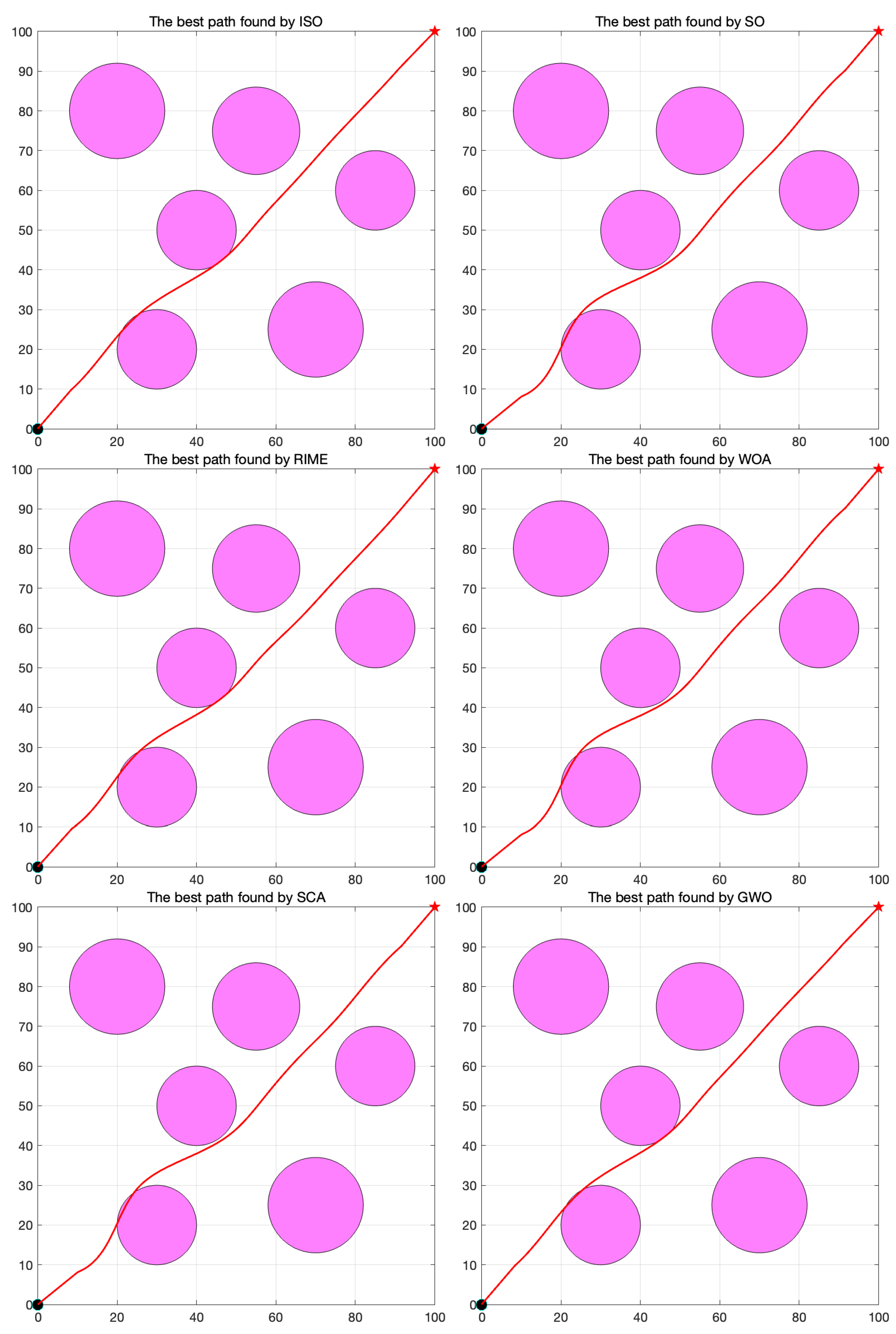
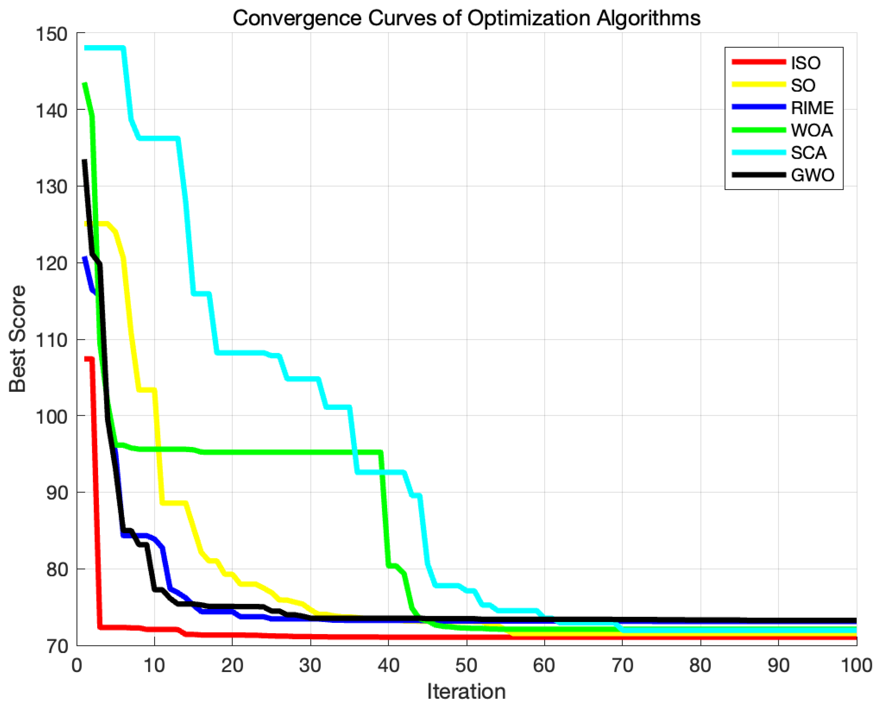
Figure 11.
Visual Comparison of UAV Path Planning
Figure 12.
Convergence Curves of Optimization Algorithms
Table 4.
Precision Data
| ISO | SO | RIME | GWO | SCA | WOA |
|---|---|---|---|---|---|
| 70.892 | 73.207 | 73.151 | 72.152 | 74.522 | 73.133 |
The ISO path is notably smoother than competing algorithms, and the algorithm converges faster. The revamped approach enhances its effectiveness in addressing 2D unmanned aerial vehicle path planning problems.
7.2. Robot Path Planning
Mobile robots play an important role in a wide range of fields such as the automation industry [59], military security [60], agricultural operations [61], mining exploration [62], and warehouse management [63]. One of their core tasks is path planning, which aims to comprehensively consider the geometric dimensions, physical limitations, and time efficiency of the robot, and plan a collision-free and optimized travel route in complex working environments [64]. Unlike motion planning, which delves into dynamic characteristics, path planning focuses more on finding a path that minimizes travel time and accurately reflects environmental features from a kinematic perspective.
To achieve this goal, robots need to construct or receive spatial models of their operating environment. These models can be explicit, actively created and stored by the robots [65], or implicit, indirectly utilized through algorithms. These spatial models can exist in various forms, including discretized representations such as grid maps, where space is uniformly divided into small blocks, or non-uniform discretization forms such as topological maps, which focus more on representing critical paths and the connection relationships between nodes. Additionally, there are continuous mapping methods that accurately describe the environment by defining a continuous coordinate sequence of polygon boundaries and paths around the boundaries. Although this method is more efficient in memory usage, in the field of robot path planning, discretized maps are favored for their ability to naturally transform into graph structures. The graph structure not only intuitively reflects environmental characteristics, but also benefits from the rich search and optimization algorithm resources in the field of graph theory, making the calculation process both efficient and concise. Therefore, although continuous mapping has its unique advantages, in practical operation, discretized maps are still the mainstream choice for robot path planning [66].
In this experiment, a robot walking on the ground is regarded as a particle of negligible size. Primary considerations encompass the intricate obstacle space and the optimization of the fitness function. The upper limit of the iteration count is set to T = 100 and the population size to N = 15.To simultaneously assess the feasibility and convergence performance of the algorithm, this experiment simulated a complex spatial environment for the robot.The detailed description is as follows: The matrix G provided undergoes a sequence of operations to produce a new matrix G. These operations are outlined as follows: The initial matrix G, with dimensions m à n, is extended by transposing it and vertically concatenating it with itself:
Matrix Extension: The initial matrix G, sized , is extended by transposing and vertically concatenating it with itself:
where denotes the transpose of G. Further Extension The resultant matrix , now sized , is further extended by transposing and vertically concatenating it with itself again:
resulting in a matrix of size . Matrix Flipping The extended matrix undergoes a flipping operation where the upper half rows are swapped with the corresponding lower half rows:
where num is the total number of rows in . Through these operations, the initial matrix G is transformed into the matrix , simulating the complex and challenging obstacle space We define the fitness function that evaluates each path by checking if the path passes through an obstacle and by calculating the total length of the path. Starting Point End Point Definition:
- The start point S is fixed to the upper left corner of the map .
- The end point E is the lower right corner of the map , where G is a matrix of size . Path definition: A path consists of a start point S, a midpoint x and an end point E:
where x is a series of coordinate points representing the intermediate path points from the start point to the end point.
Obstacle Checking: Each point in the path is checked and the number of obstacles the path passes through is calculated :
Path length calculation: If the path does not pass through any obstacle, i.e. , a smooth path is generated and the total length of the path is calculated:
Collision penalty: If the path passes through an obstacle, i.e. , the adaptation value is the map area multiplied by the number of collisions:
The fitness function: Combining the above, the final form of the fitness function is:
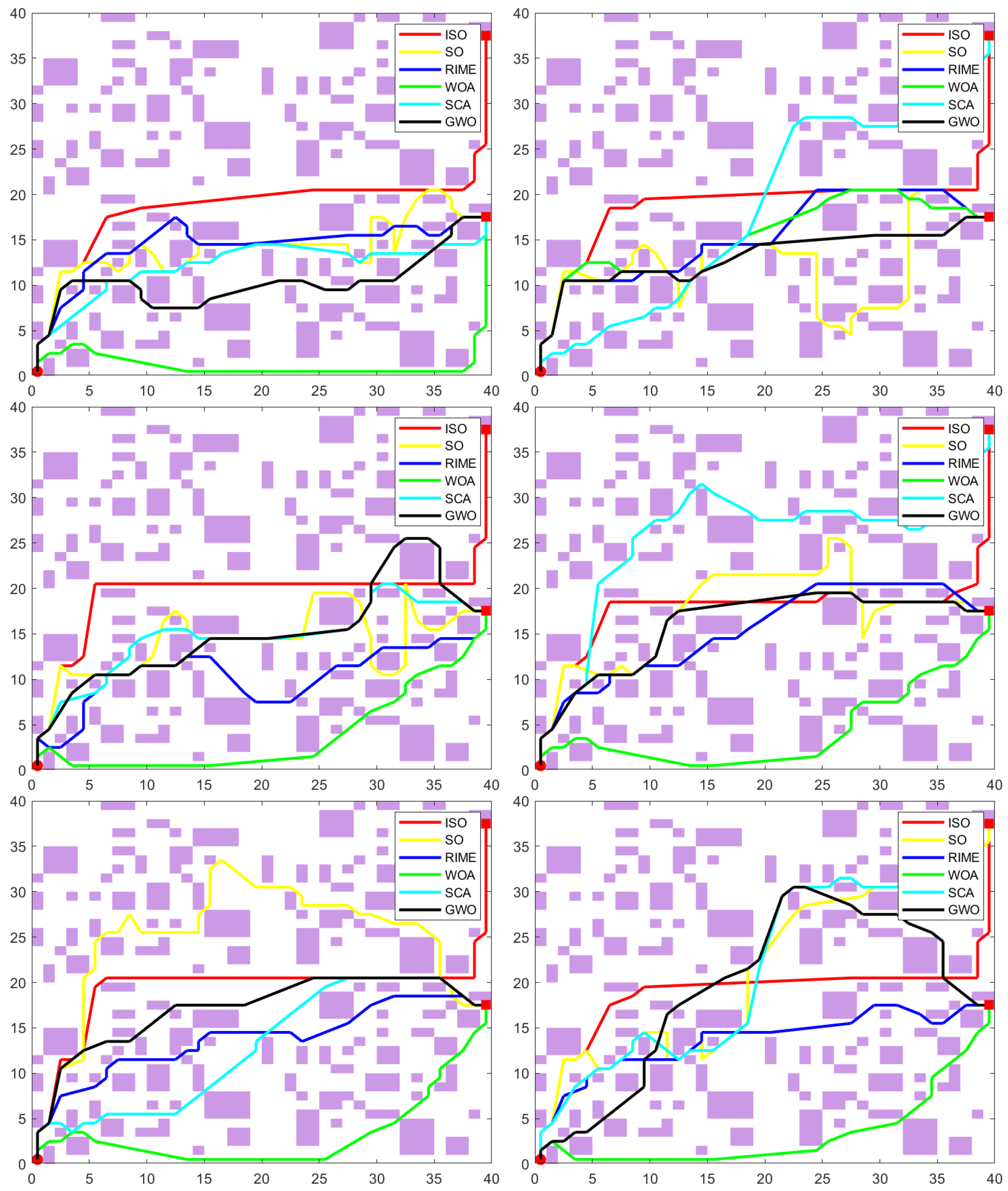
Figure 13.
Visual Comparison of robot path planning in complex scenarios
Table 5.
Precision Data
| Experiment | ISO | SO | RIME | WOA | SCA | GWO |
| 1 | Success (68.4081) | Failure (71.0511) | Failure (53.4309) | Failure (57.3173) | Failure (83.4763) | Failure (53.6302) |
| 2 | Success (70.0802) | Failure (85.3329) | Failure (54.1934) | Failure (53.826) | Success (87.9804) | Failure (50.4595) |
| 3 | Success (72.376) | Failure (79.9242) | Failure (56.6274) | Failure (49.7342) | Failure (80.1427) | Failure (59.6362) |
| 4 | Success (71.117) | Failure (71.9905) | Failure (51.5289) | Failure (51.3301) | Success (80.7291) | Failure (51.0745) |
| 5 | Success (71.799) | Failure (79.826) | Failure (50.7607) | Failure (50.8605) | Failure (76.9859) | Failure (52.1692) |
| 6 | Success (69.3769) | Success (81.929) | Failure (50.8476) | Failure (50.207) | Success (91.7876) | Failure (64.3891) |
Through data analysis, it can be demonstrated that ISO surpasses SO and four other competing algorithms when facing complex optimization spaces, boasting a 100% success rate in search, showcasing superior adaptability and robustness. Furthermore, in successfully completing tasks, Compared to SO, ISO reduces the robot’s path length by 15.4%, and compared to SCA, ISO reduces the robot’s path length by 19.1% on average.
7.3. Wireless Sensor Network Node Deployment
With the development of distributed environments such as grid computing[67,68,69], peer-to-peer networks[70,71,72] and cloud computing[73,74,75] ,wireless sensor networks (WSNs) have become more popular than ever. WSNs represent an emerging computing and networking paradigm that can be defined as networks composed of miniature, small, inexpensive, and highly intelligent devices known as sensor nodes.[76] In Wireless sensor network node deployment,We deploy n wireless sensor nodes in a two-dimensional planar region A[77]. Each node can obtain its position and has an identical sensing radius R. The sensing radius R denotes the maximum distance a sensor node can detect, meaning all points within a circular area centered at node with radius R are covered by this node. Our objective is to optimize the distribution of nodes to maximize the proportion of the area that is covered. For this problem, set the maximum iteration count T = 500 and the population size N = 200.
Let represent all WSN nodes in region A, where denotes the coordinates of node in A. For any grid point ( ), with coordinates , the distance between node and grid point is given by:
The coverage of grid point by node is described by:
Where R is the sensing radius of the sensor, varying for different types of sensors (4, 6, 8).
Define an matrix M where each element indicates whether the corresponding grid point is covered. Initially, all elements of M are 0. For each node , compute all grid points it covers and set the corresponding elements in M to 1. The coverage rate is defined as the ratio of covered grid points to the total number of grid points:
Our optimization objective is to maximize the coverage rate . Since represents the proportion of the covered area, the optimization problem can be formulated as:
We conducted tests using three different sensing radii, validating the algorithm’s performance and robustness in optimizing wireless network coverage under varying radii:
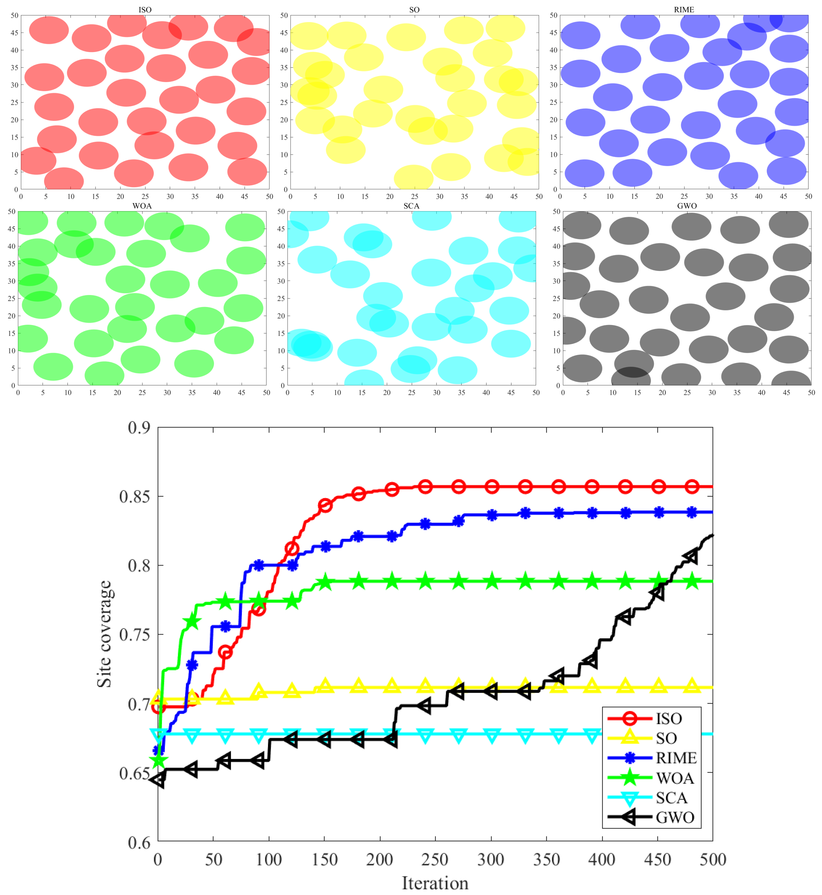
Figure 14.
The Coverage Effectiveness and Convergence Curves of Sensor Wireless Network Coverage.
Table 6.
Precision Data
| ISO | SO | RIME | GWO | SCA | WOA |
|---|---|---|---|---|---|
| 0.8571 | 0.71137 | 0.83802 | 0.78817 | 0.67697 | 0.80669 |
Qualitative analysis of six maps of wireless network coverage shows that ISO , compared to SO and four other competing algorithms, consistently achieves more uniform coverage. Additionally, quantitative evidence from convergence curve graphs confirms that ISO exhibits stronger solving capabilities compared to competing algorithms, resulting in the attainment of the maximum network coverage area.
7.3.1. Pressure Vessel Design
Pressure vessels are widely used where it is required to hold the fluids at high pressure as well as temperature.[78] They are majorly used in processing plants, nuclear power plants, and oil refining industries. The Pressure Vessel Design(PVD) problem features a structure as shown in Fig. 18. Our design philosophy is to maximize cost-effectiveness while fully meeting practical application needs, by finely adjusting four key parameters to achieve this goal.[79] These four crucial optimization dimensions are: vascular thickness (), head thickness (), inner radius (R), and head length (L). In order to quantify and optimize the comprehensive impact of these parameters, we have constructed an accurate mathematical model, as shown in Equation (21). This model not only reflects the complex relationship between design parameters and performance, but also provides us with a scientific basis for optimizing design, ensuring effective control and reduction of overall costs while meeting usage requirements.
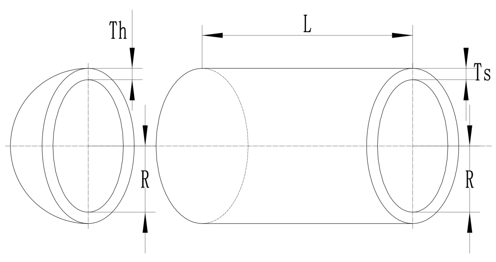
Figure 15.
Pressure Vessel Design
Table 7.
Optimal values for Variables and Their Corresponding Optimal Value and Ranking for Different Algorithms.
Table 7.
Optimal values for Variables and Their Corresponding Optimal Value and Ranking for Different Algorithms.
| Algorithm | h | l | t | b | Optimal value | Ranking |
| ISO | 0.1991 | 3.3339 | 9.1857 | 0.1991 | 1.6712 | 1 |
| SO | 0.19372 | 3.437 | 9.192 | 0.19883 | 1.6757 | 2 |
| RIME | 0.4176 | 2.3298 | 4.9704 | 0.68011 | 3.1046 | 6 |
| SCA | 0.19728 | 3.8021 | 9.181 | 0.19971 | 1.7338 | 4 |
| GWO | 0.1942 | 3.4412 | 9.1891 | 0.19897 | 1.6776 | 3 |
| WOA | 0.125 | 8.3518 | 8.3518 | 0.24085 | 2.3073 | 5 |
From the results in Table 17, it is evident that ISO outperform all other competitors, achieving a minimum cost of 1.6712.
8. Conclusion and Outlook
This paper introduces the Improved Snake Optimization Algorithm (ISO), an advanced metaheuristic algorithm.While the original Snake Optimization Algorithm (SO) has been praised for its effectiveness in certain problem domains.It encounters slow convergence and frequently gets trapped in local optima.To overcome these limitations, ISO optimizes the initial population distribution using the Sobol sequence and enhances convergence speed and global search capability by incorporating elements from the Rime Optimization Algorithm (RIME) and lens imaging-based reverse learning. To validate the performance of ISO, we quantitatively analyzed population initialization using Star Discrepancy, Average Nearest Neighbor Distance, and Sum of Squared Deviations, and assessed its exploration and exploitation capabilities using CEC2017. The results indicate that ISO possesses an excellent and uniform initial population distribution and can maintain a balance between exploration and exploitation. Subsequently, extensive evaluations using 23 benchmark functions, including unimodal, multimodal, hybrid, and composite functions, were conducted. The effectiveness of the results was validated using Wilcoxon rank-sum tests. These demonstrate ISOâs superior performance in terms of convergence speed, stability, and solution quality. Furthermore, ISO’s practical applicability is validated through its successful deployment in complex engineering tasks such as UAV path planning, robotic path planning, wireless network layout optimization and Pressure vessel design . The results consistently show that ISO outperforms comparative algorithms, finding better solutions more efficiently. This work significantly advances the field of optimization algorithms, offering a robust and efficient solution for complex real-world problems and demonstrating ISO’s immense potential for future research and engineering applications. Overall, the Fusion of RIME Algorithm Improved Snake Optimization Algorithm has demonstrated excellent solving performance in population diversity and exploration and development testing in Section 5, benchmark function testing in Section 6, and extensive engineering problem testing in Section 7. This indicates that ISO can provide a more uniform initial population distribution and maintain a balance between exploration and development in up to 500 algorithm iterations when solving problems. It is capable of handling complex and diverse benchmark function testing, has strong robustness, and can cope with engineering problem challenges in different scenarios. Although ISO algorithm has demonstrated strong convergence ability and robustness in the performance tests of three sections, there is still more room for improvement in the future for us to explore. The improvement and upgrading of meta heuristic algorithms mainly involve three levels.
1. Diversification strategy: Integrating and/or to propose more strategies,including classical metaheuristic algorithm strategies[80,81]and innovative machine learning strategies[82,83] and discussing these strategies, on the one hand, to find the best strategy, and on the other hand, to make a trade-off between the performance improvement and computational loss brought by these strategies to the algorithm.
2.Extensive performance testing: For metaheuristic algorithms, an optimal population distribution [84] and a balance between exploration and exploitation[85] are crucial performance indicators. It is necessary to apply and/or propose more effective analytical methods for a comprehensive analysis of metaheuristic algorithms.At the benchmark function level[86], apply and/or propose test functions such as cec2014 and cec2022[87], and discuss which functions among the existing and/or proposed test functions can truly verify the solving performance of the meta heuristic algorithm. Different test functions specifically examine the ability of the meta heuristic algorithm on one hand, which is conducive to scholars selecting the most suitable test function from up to hundreds of test functions and/or proposing more targeted test functions. At the practical application level[88], algorithm testing should not only be conducted on classic engineering problems, but also applied to a wider range of engineering problems. The algorithm should be compared not only with meta heuristic algorithms, but also with other non deterministic algorithms and/or deterministic algorithms to deeply explore which algorithm is most suitable for solving real-world problems[89].
3.Combining quantum computing: Quantum computing is an emerging and thriving scientific technology[90,91]. So far, many scholars have pioneered the combination of metaheuristic algorithms with quantum computing and have proven that it leads classical metaheuristic algorithms in various problems. The integration of metaheuristic algorithms with quantum computing occurs at three levels[92], which can be classified into quantum inspired metaheuristic algorithms, quantum simulation metaheuristic algorithms, and real quantum metaheuristic algorithms. The discussion on quantum inspired metaheuristic algorithms[93,94] has been ongoing for 20 years. Inspired by the uncertainty in quantum behavior, this algorithm incorporates probabilistic or chaotic strategies into metaheuristic algorithms.Although it mimics some quantum behavior, it still belongs to the classical category. The category of metaheuristic algorithms includes quantum simulation metaheuristic algorithms and real quantum metaheuristic algorithms. This field has only emerged in recent years[95], using quantum computing principles based on quantum mechanics to mathematically model metaheuristic algorithms and problems applicable to metaheuristic algorithms, and solving problems under new models. The former uses classical computer simulation to solve the process, which allows researchers to study and verify the effectiveness and potential applications of quantum algorithms without the need for actual quantum hardware, while the latter’s solving process occurs on real quantum computers. Researchers who deeply understand and combine quantum computing with metaheuristic algorithms will design algorithms that are more efficient and have potential than ever before. Meanwhile, this will be an open and meaningful field[96].
References
- J. Tang, G. Liu, and Q. T. Pan, "A Review on Representative Swarm Intelligence Algorithms for Solving Optimization Problems: Applications and Trends," IEEE/CAA J. Autom. Sinica, vol. 8, no. 10, pp. 1627-1643, Oct. 2021. [CrossRef]
- Breiman, L., Cutler, A. A deterministic algorithm for global optimization. Mathematical Programming 58, 179â199 (1993). [CrossRef]
- Tansel Dokeroglu, Ender Sevinc, Tayfun Kucukyilmaz, Ahmet Cosar,A survey on new generation metaheuristic algorithms,Computers & Industrial Engineering,Volume 137,2019,106040,ISSN 0360-8352. [CrossRef]
- P. Agrawal, H. F. Abutarboush, T. Ganesh and A. W. Mohamed, "Metaheuristic Algorithms on Feature Selection: A Survey of One Decade of Research (2009-2019)," in IEEE Access, vol. 9, pp. 26766-26791, 2021. [CrossRef]
- Adam, S. P., Alexandropoulos, S. A. N., Pardalos, P. M., & Vrahatis, M. N. (2019). No free lunch theorem: A review. Approximation and optimization: Algorithms, complexity and applications, 57-82. [CrossRef]
- Fatma A. Hashim, Abdelazim G. Hussien,Snake Optimizer: A novel meta-heuristic optimization algorithm,KnowledgeBasedSystems,Volume 242,2022,108320. [CrossRef]
- Peng, L., Yuan, Z., Dai, G. et al. A Multi-strategy Improved Snake Optimizer Assisted with Population Crowding Analysis for Engineering Design Problems. J Bionic Eng 21, 1567â1591 (2024). [CrossRef]
- Tsakiridis, N. L., Theocharis, J. B., & Zalidis, G. C. (2016). DECO3R: A Differential Evolution-based algorithm for generating compact Fuzzy Rule-based Classification Systems. Knowledge-Based Systems, 105, 160-174. [CrossRef]
- Su, H., Zhao, D., Heidari, A. A., Liu, L., Zhang, X., Mafarja, M., & Chen, H. (2023). RIME: A physics-based optimization. Neurocomputing, 532, 183-214. [CrossRef]
- Fattahi, E., Bidar, M., & Kanan, H. R. (2018). Focus group: an optimization algorithm inspired by human behavior. International Journal of Computational Intelligence and Applications, 17(01), 1850002. [CrossRef]
- Chakraborty A, Kar A K. Swarm intelligence: A review of algorithms[J]. Nature-inspired computing and optimization: Theory and applications, 2017: 475-494. [CrossRef]
- Mirjalili S, Mirjalili S. Genetic algorithm[J]. Evolutionary algorithms and neural networks: Theory and applications, 2019: 43-55. [CrossRef]
- Espejo P G, Ventura S, Herrera F. A survey on the application of genetic programming to classification[J]. IEEE Transactions on Systems, Man, and Cybernetics, Part C (Applications and Reviews), 2009, 40(2): 121-144. [CrossRef]
- Maheri A, Jalili S, Hosseinzadeh Y, et al. A comprehensive survey on cultural algorithms[J]. Swarm and Evolutionary Computation, 2021, 62: 100846. [CrossRef]
- Bertsimas, D., & Tsitsiklis, J. (1993). Simulated annealing. Statistical science, 8(1), 10-15. [CrossRef]
- Kennedy, J., & Eberhart, R. (1995, November). Particle swarm optimization. In Proceedings of ICNN’95-international conference on neural networks (Vol. 4, pp. 1942-1948). ieee.
- Han, K. H., & Kim, J. H. (2002). Quantum-inspired evolutionary algorithm for a class of combinatorial optimization. IEEE transactions on evolutionary computation, 6(6), 580-593. [CrossRef]
- Xu, L. D. (1994). Case based reasoning. IEEE potentials, 13(5), 10-13. [CrossRef]
- Qiang, W., & Zhongli, Z. (2011, August). Reinforcement learning model, algorithms and its application. In 2011 International Conference on Mechatronic Science, Electric Engineering and Computer (MEC) (pp. 1143-1146). IEEE.
- Dorigo, M., & Stützle, T. (2019). Ant colony optimization: overview and recent advances (pp. 311-351). Springer International Publishing.
- Abualigah, L., Shehab, M., Alshinwan, M., & Alabool, H. (2020). Salp swarm algorithm: a comprehensive survey. Neural Computing and Applications, 32(15), 11195-11215. [CrossRef]
- Hashim, F. A., & Hussien, A. G. (2022). Snake Optimizer: A novel meta-heuristic optimization algorithm. Knowledge-Based Systems, 242, 108320. [CrossRef]
- Yan, C., & Razmjooy, N. (2023). Optimal lung cancer detection based on CNN optimized and improved Snake optimization algorithm. Biomedical Signal Processing and Control, 86, 105319. [CrossRef]
- Zheng, W., Pang, S., Liu, N., Chai, Q., & Xu, L. (2023). A compact snake optimization algorithm in the application of WKNN fingerprint localization. Sensors, 23(14), 6282. [CrossRef]
- Hu, G., Yang, R., Abbas, M., & Wei, G. (2023). BEESO: Multi-strategy boosted snake-inspired optimizer for engineering applications. Journal of Bionic Engineering, 20(4), 1791-1827. [CrossRef]
- Osuna-Enciso, V., Cuevas, E., & Castañeda, B. M. (2022). A diversity metric for population-based metaheuristic algorithms. Information Sciences, 586, 192-208. [CrossRef]
- Agushaka, J. O., & Ezugwu, A. E. (2022). Initialisation approaches for population-based metaheuristic algorithms: a comprehensive review. Applied Sciences, 12(2), 896. [CrossRef]
- Joe, S., & Kuo, F. Y. (2008). Constructing Sobol sequences with better two-dimensional projections. SIAM Journal on Scientific Computing, 30(5), 2635-2654. [CrossRef]
- Su, H., Zhao, D., Heidari, A. A., Liu, L., Zhang, X., Mafarja, M., & Chen, H. (2023). RIME: A physics-based optimization. Neurocomputing, 532, 183-214. [CrossRef]
- Zhong, R., Yu, J., Zhang, C., & Munetomo, M. (2024). SRIME: a strengthened RIME with Latin hypercube sampling and embedded distance-based selection for engineering optimization problems. Neural Computing and Applications, 36(12), 6721-6740. [CrossRef]
- Osuna-Enciso, V., Cuevas, E., & Castañeda, B. M. (2022). A diversity metric for population-based metaheuristic algorithms. Information Sciences, 586, 192-208. [CrossRef]
- Learning, L. (2021). Image Formation by Lenses. Fundamentals of Heat, Light & Sound.
- Ouyang, C., Zhu, D., & Qiu, Y. (2021). Lens learning sparrow search algorithm. Mathematical Problems in Engineering, 2021(1), 9935090. [CrossRef]
- Osuna-Enciso, V., Cuevas, E., & Castañeda, B. M. (2022). A diversity metric for population-based metaheuristic algorithms. Information Sciences, 586, 192-208. [CrossRef]
- Cuevas, E., Luque, A., Morales Castañeda, B., & Rivera, B. (2024). A Measure of Diversity for Metaheuristic Algorithms Employing Population-Based Approaches. In Metaheuristic Algorithms: New Methods, Evaluation, and Performance Analysis (pp. 49-72). Cham: Springer Nature Switzerland.
- Cuevas, E., Diaz, P., Camarena, O., Cuevas, E., Diaz, P., & Camarena, O. (2021). Experimental analysis between exploration and exploitation. Metaheuristic Computation: A Performance Perspective, 249-269. [CrossRef]
- Yang, X. S., Deb, S., & Fong, S. (2014). Metaheuristic algorithms: optimal balance of intensification and diversification. Applied Mathematics & Information Sciences, 8(3), 977. [CrossRef]
- Clément, F., Doerr, C., & Paquete, L. (2022). Star discrepancy subset selection: Problem formulation and efficient approaches for low dimensions. Journal of Complexity, 70, 101645. [CrossRef]
- Thiémard, E. (2001). An algorithm to compute bounds for the star discrepancy. journal of complexity, 17(4), 850-880. [CrossRef]
- Bansal, P. P., & Ardell, A. J. (1972). Average nearest-neighbor distances between uniformly distributed finite particles. Metallography, 5(2), 97-111. [CrossRef]
- Kobayashi, K., & Salam, M. U. (2000). Comparing simulated and measured values using mean squared deviation and its components. Agronomy Journal, 92(2), 345-352. [CrossRef]
- Salleh, M. N. M., Hussain, K., Cheng, S., Shi, Y., Muhammad, A., Ullah, G., & Naseem, R. (2018). Exploration and exploitation measurement in swarm-based metaheuristic algorithms: An empirical analysis. In Recent Advances on Soft Computing and Data Mining: Proceedings of the Third International Conference on Soft Computing and Data Mining (SCDM 2018), Johor, Malaysia, February 06-07, 2018 (pp. 24-32). Springer International Publishing.
- Mirjalili, S. (2016). SCA: a sine cosine algorithm for solving optimization problems. Knowledge-based systems, 96, 120-133. [CrossRef]
- Mirjalili, S., & Lewis, A. (2016). The whale optimization algorithm. Advances in engineering software, 95, 51-67. [CrossRef]
- Mirjalili, S., Mirjalili, S. M., & Lewis, A. (2014). Grey wolf optimizer. Advances in engineering software, 69, 46-61. [CrossRef]
- Garcà a-Martà nez, C., Gutiérrez, P. D., Molina, D., Lozano, M., & Herrera, F. (2017). Since CEC 2005 competition on real-parameter optimisation: a decade of research, progress and comparative analysisâs weakness. Soft Computing, 21, 5573-5583. [CrossRef]
- Sun, Y., & Genton, M. G. (2011). Functional boxplots. Journal of Computational and Graphical Statistics, 20(2), 316-334. [CrossRef]
- Wilcoxon, F., Katti, S., & Wilcox, R. A. (1970). Critical values and probability levels for the Wilcoxon rank sum test and the Wilcoxon signed rank test. Selected tables in mathematical statistics, 1, 171-259.
- Tsouros, D. C., Bibi, S., & Sarigiannidis, P. G. (2019). A review on UAV-based applications for precision agriculture. Information, 10(11), 349.(6), 4233-4284. [CrossRef]
- Delavarpour, N., Koparan, C., Nowatzki, J., Bajwa, S., & Sun, X. (2021). A technical study on UAV characteristics for precision agriculture applications and associated practical challenges. Remote Sensing, 13(6), 1204. [CrossRef]
- Yang, L., Fan, J., Liu, Y., Li, E., Peng, J., & Liang, Z. (2020). A review on state-of-the-art power line inspection techniques. IEEE Transactions on Instrumentation and Measurement, 69(12), 9350-9365. [CrossRef]
- Zhang, Y., Yuan, X., Li, W., & Chen, S. (2017). Automatic power line inspection using UAV images. Remote Sensing, 9(8), 824. [CrossRef]
- Li, X., & Yang, L. (2012, August). Design and implementation of UAV intelligent aerial photography system. In 2012 4th International Conference on Intelligent Human-Machine Systems and Cybernetics (Vol. 2, pp. 200-203). IEEE.
- ZHANG, J. (2021). Review of the light-weighted and small UAV system for aerial photography and remote sensing. National Remote Sensing Bulletin, 25(3), 708-724. [CrossRef]
- Lyu, C., & Zhan, R. (2022). Global analysis of active defense technologies for unmanned aerial vehicle. IEEE Aerospace and Electronic Systems Magazine, 37(1), 6-31. [CrossRef]
- .
- Roberge, V., Tarbouchi, M., & Labonté, G. (2012). Comparison of parallel genetic algorithm and particle swarm optimization for real-time UAV path planning. IEEE Transactions on industrial informatics, 9(1), 132-141. [CrossRef]
- Puente-Castro, A., Rivero, D., Pazos, A., & Fernandez-Blanco, E. (2022). A review of artificial intelligence applied to path planning in UAV swarms. Neural Computing and Applications, 34(1), 153-170. [CrossRef]
- Mac, T. T., Copot, C., Tran, D. T., & De Keyser, R. (2016). Heuristic approaches in robot path planning: A survey. Robotics and Autonomous Systems, 86, 13-28. [CrossRef]
- Zhang, H., Wang, Y., Zheng, J., & Yu, J. (2018). Path planning of industrial robot based on improved RRT algorithm in complex environments. IEEE Access, 6, 53296-53306. [CrossRef]
- Kunchev, V., Jain, L., Ivancevic, V., & Finn, A. (2006). Path planning and obstacle avoidance for autonomous mobile robots: A review. In Knowledge-Based Intelligent Information and Engineering Systems: 10th International Conference, KES 2006, Bournemouth, UK, October 9-11, 2006. Proceedings, Part II 10 (pp. 537-544). Springer Berlin Heidelberg.
- Chakraborty, S., Elangovan, D., Govindarajan, P. L., ELnaggar, M. F., Alrashed, M. M., & Kamel, S. (2022). A comprehensive review of path planning for agricultural ground robots. Sustainability, 14(15), 9156. [CrossRef]
- Weimin, Z. H. A. N. G., Yue, Z. H. A. N. G., & Hui, Z. H. A. N. G. (2022). Path planning of coal mine rescue robot based on improved A* algorithm. Coal Geology & Exploration, 50(12), 20. [CrossRef]
- Vivaldini, K. C., Galdames, J. P., Bueno, T. S., Araújo, R. C., Sobral, R. M., Becker, M., & Caurin, G. A. (2010, March). Robotic forklifts for intelligent warehouses: Routing, path planning, and auto-localization. In 2010 IEEE International Conference on Industrial Technology (pp. 1463-1468). IEEE.
- Raja, P., & Pugazhenthi, S. (2012). Optimal path planning of mobile robots: A review. International journal of physical sciences, 7(9), 1314-1320. [CrossRef]
- Souissi, O., Benatitallah, R., Duvivier, D., Artiba, A., Belanger, N., & Feyzeau, P. (2013, October). Path planning: A 2013 survey. In Proceedings of 2013 international conference on industrial engineering and systems management (IESM) (pp. 1-8). IEEE.
- Lim, H. B., Teo, Y. M., Mukherjee, P., Lam, V. T., Wong, W. F., & See, S. (2005, November). Sensor grid: Integration of wireless sensor networks and the grid. In The IEEE Conference on Local Computer Networks 30th Anniversary (LCN’05) l (pp. 91-99). IEEE.
- Sanchez-Ibanez, J. R., Pérez-del-Pulgar, C. J., & Garcà a-Cerezo, A. (2021). Path planning for autonomous mobile robots: A review. Sensors, 21(23), 7898. [CrossRef]
- Farman, H., Javed, H., Ahmad, J., Jan, B., & Zeeshan, M. (2016). Gridâbased hybrid network deployment approach for energy efficient wireless sensor networks. Journal of Sensors, 2016(1), 2326917. [CrossRef]
- Lim, H. B., Teo, Y. M., Mukherjee, P., Lam, V. T., Wong, W. F., & See, S. (2005, November). Sensor grid: Integration of wireless sensor networks and the grid. In The IEEE Conference on Local Computer Networks 30th Anniversary (LCN’05) l (pp. 91-99). IEEE.
- Carbajo, R. S., & Mc Goldrick, C. (2017). Decentralised peer-to-peer data dissemination in wireless sensor networks. Pervasive and Mobile Computing, 40, 242-266. [CrossRef]
- KrÄo, S., Cleary, D., & Parker, D. (2005). Enabling ubiquitous sensor networking over mobile networks through peer-to-peer overlay networking. Computer communications, 28(13), 1586-1601. [CrossRef]
- Park, H., & Hutchinson, S. (2014, May). Robust optimal deployment in mobile sensor networks with peer-to-peer communication. In 2014 IEEE International Conference on Robotics and Automation (ICRA) (pp. 2144-2149). IEEE.
- Dash, S. K., Mohapatra, S., & Pattnaik, P. K. (2010). A survey on applications of wireless sensor network using cloud computing. International Journal of Computer Science & Emerging Technologies, 1(4), 50-55.
- Ahmed, K., & Gregory, M. (2011, December). Integrating wireless sensor networks with cloud computing. In 2011 seventh international conference on mobile ad-hoc and sensor networks (pp. 364-366). IEEE.
- Elamin, W. M., Endan, J. B., Yosuf, Y. A., Shamsudin, R., & Ahmedov, A. (2015). High pressure processing technology and equipment evolution: a review. Journal of Engineering Science & Technology Review, 8(5). [CrossRef]
- Ballesteros, A., Ahlstrand, R., Bruynooghe, C., Von Estorff, U., & Debarberis, L. (2012). The role of pressure vessel embrittlement in the long term operation of nuclear power plants. Nuclear engineering and design, 243, 63-68. [CrossRef]
- Chen, X., Fan, Z., Chen, Y., Zhang, X., Cui, J., Zheng, J., & Shou, B. (2018, July). Development of lightweight design and manufacture of heavy-duty pressure vessels in China. In Pressure Vessels and Piping Conference (Vol. 51593, p. V01BT01A023). American Society of Mechanical Engineers.
- Khanduja, N., & Bhushan, B. (2021). Recent advances and application of metaheuristic algorithms: A survey (2014â2020). Metaheuristic and evolutionary computation: algorithms and applications, 207-228. [CrossRef]
- Yaghoubzadeh-Bavandpour, A., Bozorg-Haddad, O., Zolghadr-Asli, B., & Gandomi, A. H. (2022). Improving approaches for meta-heuristic algorithms: A brief overview. Computational Intelligence for Water and Environmental Sciences, 35-61. [CrossRef]
- Talbi, E. G. (2021). Machine learning into metaheuristics: A survey and taxonomy. ACM Computing Surveys (CSUR), 54(6), 1-32. [CrossRef]
- Chiroma, H., Gital, A. Y. U., Rana, N., Abdulhamid, S. I. M., Muhammad, A. N., Umar, A. Y., & Abubakar, A. I. (2020). Nature inspired meta-heuristic algorithms for deep learning: recent progress and novel perspective. In Advances in Computer Vision: Proceedings of the 2019 Computer Vision Conference (CVC), Volume 1 1 (pp. 59-70). Springer International Publishing.
- da Costa Oliveira, A. L., Britto, A., & Gusmão, R. (2023). Machine learning enhancing metaheuristics: a systematic review. Soft Computing, 27(21), 15971-15998. [CrossRef]
- Hassanzadeh, M. R., & Keynia, F. (2021). An overview of the concepts, classifications, and methods of population initialization in metaheuristic algorithms. Journal of Advances in Computer Engineering and Technology, 7(1), 35-54.
- Han, Y., Chen, W., Heidari, A. A., Chen, H., & Zhang, X. (2024). Balancing ExplorationâExploitation of Multi-verse Optimizer for Parameter Extraction on Photovoltaic Models. Journal of Bionic Engineering, 21(2), 1022-1054. [CrossRef]
- Sharma, P., & Raju, S. (2024). Metaheuristic optimization algorithms: A comprehensive overview and classification of benchmark test functions. Soft Computing, 28(4), 3123-3186. [CrossRef]
- Hussain, K., Salleh, M. N. M., Cheng, S., & Naseem, R. (2017). Common benchmark functions for metaheuristic evaluation: A review. JOIV: International Journal on Informatics Visualization, 1(4-2), 218-223. [CrossRef]
- Yang, X. S. (2010). Engineering optimization: an introduction with metaheuristic applications. John Wiley & Sons.
- Bozorg-Haddad, O., Solgi, M., & Loáiciga, H. A. (2017). Meta-heuristic and evolutionary algorithms for engineering optimization. John Wiley & Sons.
- Hidary, J. D., & Hidary, J. D. (2019). Quantum computing: an applied approach (Vol. 1). Cham: Springer.
- Fauseweh, B. (2024). Quantum many-body simulations on digital quantum computers: State-of-the-art and future challenges. Nature Communications, 15(1), 2123. [CrossRef]
- Dahi, Z. A., & Alba, E. (2022). Metaheuristics on quantum computers: Inspiration, simulation and real execution. Future Generation Computer Systems, 130, 164-180. [CrossRef]
- Gharehchopogh, F. S. (2023). Quantum-inspired metaheuristic algorithms: comprehensive survey and classification. Artificial Intelligence Review, 56(6), 5479-5543. [CrossRef]
- Rylander, B., Soule, T., Foster, J. A., & Alves-Foss, J. (2000, July). Quantum Genetic Algorithms. In GECCO (p. 373).
- Ross, O. H. M. (2019). A review of quantum-inspired metaheuristics: Going from classical computers to real quantum computers. Ieee Access, 8, 814-838. [CrossRef]
- Nielsen, M6. A., & Chuang, I. L. (2010). Quantum computation and quantum information. Cambridge university press. [CrossRef]
Figure 4.
The balance between exploration and exploitation
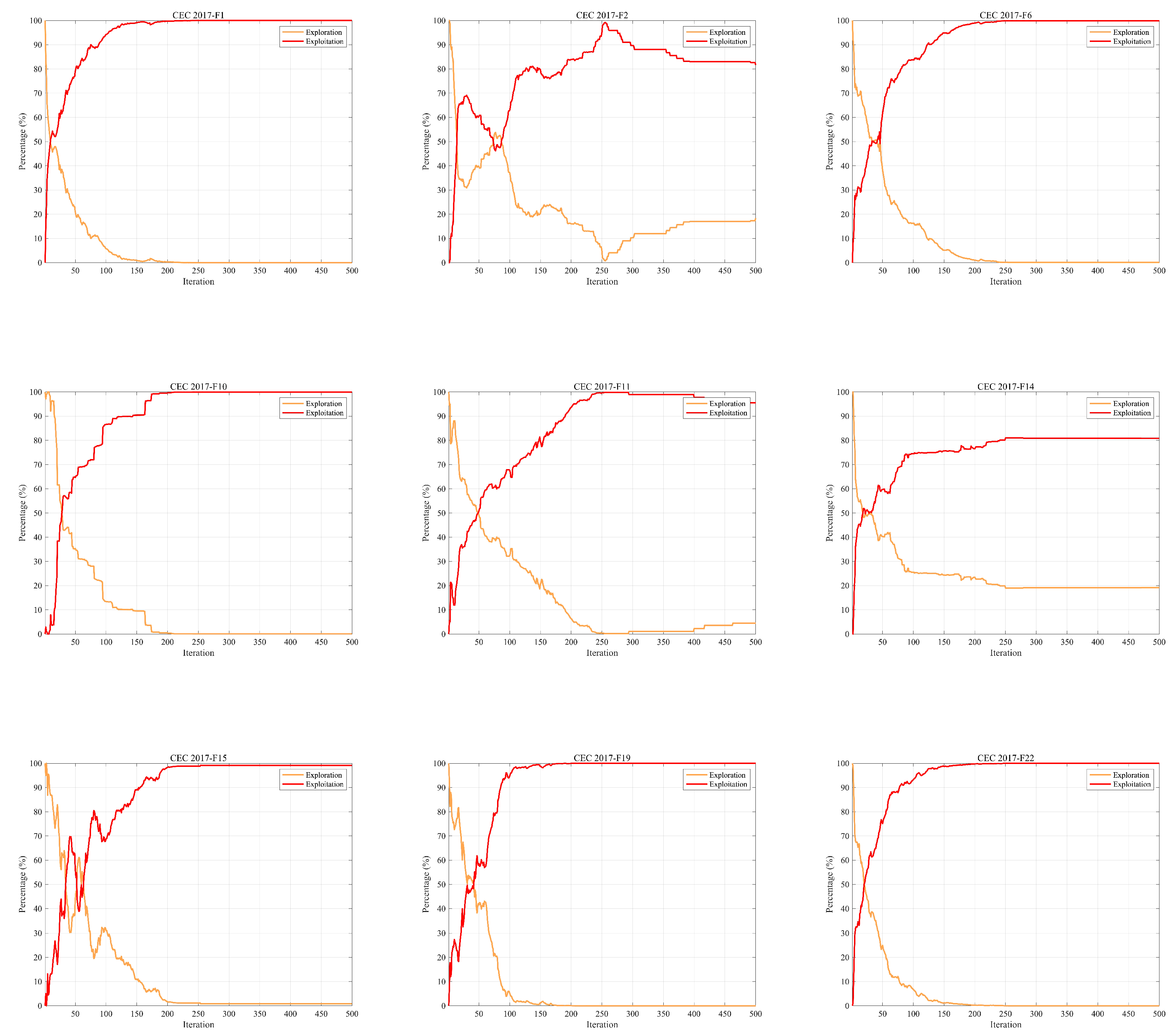
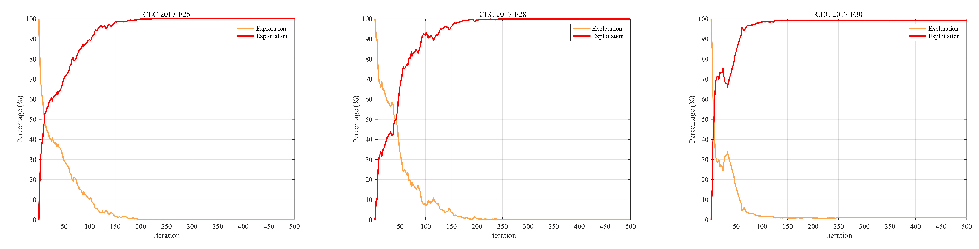
Disclaimer/Publisher’s Note: The statements, opinions and data contained in all publications are solely those of the individual author(s) and contributor(s) and not of MDPI and/or the editor(s). MDPI and/or the editor(s) disclaim responsibility for any injury to people or property resulting from any ideas, methods, instructions or products referred to in the content. |
© 2024 by the authors. Licensee MDPI, Basel, Switzerland. This article is an open access article distributed under the terms and conditions of the Creative Commons Attribution (CC BY) license (http://creativecommons.org/licenses/by/4.0/).
Copyright: This open access article is published under a Creative Commons CC BY 4.0 license, which permit the free download, distribution, and reuse, provided that the author and preprint are cited in any reuse.


