Competitive Bidding Strategy in an Auction with Random Cutoff—Randomness Is Always Unpredictable?

Jin Hyung Lee

doi:10.20944/preprints202408.0602.v1

Preprint

Article

Competitive Bidding Strategy in an Auction with Random Cutoff—Randomness Is Always Unpredictable?

This version is not peer-reviewed.

Jin Hyung Lee^*

This version is not peer-reviewed.

Downloads

Views

Comments

Submitted:

08 August 2024

Posted:

08 August 2024

You are already at the latest version

Abstract

This paper detects bidding behaviors in the auction with the random cutoff, where a winning bid needs to be above and the closest to the random cutoff. In this auction, each bidder is eager to predict the random cutoff in order to use the predicted random cutoff as bid. Furthermore, one of deep learning models, the transformer model is employed as one empirical method to anticipate the random cutoff. The result shows that the predicted random cutoff turns out to be a winner with probability of about 20 percent. This paper contributes to economic literature in terms of investigating the connection between a deep learning model and an auction based on the economic theory.

Keywords:

reverse auction

;

random cutoff

;

transformer model

Subject:

Business, Economics and Management - Economics

This preprints belongs to the Topic

Advanced Techniques and Modeling in Business and Economics

1. Introduction

The reverse auction is designed to set up a mechanism such that the most cost-efficient bidder is awarded the auction item. It is believed that this mechanism is supposed to function well in either the first price reverse auction or the second price reverse auction. Although the improvement in cost efficiency is the main interest to the reverse auction in general, the other purpose is added to this type of auction. For example, the cutoff is established in the first price reverse auction to prevent the default of a winner due to the winner’s curse induced by fierce competition. Particularly, if a bidder submits a bid below the cutoff, the bidder is disqualified. Accordingly, the winning bid should be at least above the cutoff, stopping the winning bid from declining down below the cutoff due to the fierce competition. According to Chen and Chiu [1], this type of reverse auction is adopted by local governments in Japan in the form of bid floor for most of their procurement auctions.

Meanwhile, if the cutoff is public to all bidders prior to bidding, almost all the cost-efficient bidders are the most likely to place the same bids as the cutoff since the profit margin is guaranteed by the cutoff. Thus, the most important work relevant to this auction is the authority of an auction holder to set up the cutoff. Then, there exists the likelihood such that bidders have incentive to make the work of the authority advantageous to them. It is occurred that an auction holder of this authority might be corrupted by some bidders. In response to the potential serious problem, the random cutoff is introduced to the reverse auction.

More specifically, the cutoff is randomly extracted from a certain range. The information on the realized cutoff is not disclosed to all bidders until the submission of all bids is finished. Thus, the discretionary power which an auction holder owns disappears, and bidders have no incentive to corrupt the auction holder in order to make the power operate in their favor. This type of reverse auction is widely employed by the central and local governments in South Korea.

Bidders are mainly interested in predicting what the random cutoff would be in an auction, where any bidder would be a winner submitting a bid both above and closest to the random cutoff. A bidding behavior is expected to be taken, corresponding with the prediction. However, it is extremely difficult to point out what the prediction would be due to the randomness brought about by the random cutoff, which would be a large obstacle to investigate what a bidding behavior would be at the equilibrium.

1.1. Related Literature

This paper investigates the issues to deal with the prediction of random number. The literature relevant to p-Beauty games is considered to be similar to the issues related to forecasting the random number. In the p-Beauty game, players predict a point equal to p-value times mean of numbers which players choose from a certain interval. In the game, a player who makes the smallest prediction error would be a winner. Since each player does not recognize rivals’ choices, players appear to act like predicting a random number.

In order to make a prediction, players are supposed to assume that rivals possess a variety of bounded rationalities. Thus, more rational is a player, more comprehensive is the player. In other words, a player with more rationality perceives the distribution of rivals with less rationality and more instinct compared to the player. Accordingly, the most rational player recognizes the whole distribution rivals in terms of their rationality level. In this case, the mean of players’ choices would be the weighted average depending on the distribution of rivals with respect to the rationality level. This is called the cognitive hierarchy model.(López [2], Hahn et al. [3])

In the cognitive hierarchy model mentioned above, the mean value is endogeneously determined by players’ choices. More impulsive and less reasonable is a player, more random choice does the player makes. In contrast, more rational or cognitively able is a player, more organized choice or equilibrium selection does the player make. Therefore, the mean value is seriously affected by the distribution of players with regard to the rationality level. In contras with the cognitive hierarchy model, this paper shows that the random cutoff is exogeneously determined, which is almost irrelevant to players’ choices. In line with this conjecture, the random cutoff is rarely affected by the rationality level of participants or players.

Meanwhile, there might be another assumption about players’ rationality. Particularly, a player with a specific rationality level, called k-step is supposed to perceive that all rivals possess the cognitive ability just below one-step, called (k-1)-step.(Crawford and Iriberri [4], Gill and Prowse [5]) This case is called a level-k analysis. As previously stated with the cognitive hierarchy model, the cognitive ability of either players or participants is important since the strategy of a player with arbitrary k-step is affected by other rivals with a (k-1)-step. This point of view is different from the suggestion by this paper which makes such an emphasis that the random cutoff is determined regardless of the cognitive levels of players.

Apart from the investigation of the cognitive levels, there exists a previous literature to detect bidding behaviors when a scoring rule to consider both bid price and quality is introduced to either a buyer determined auction or reverse auction. Haruvy and Jap [6] empirically demonstrate that bidding behaviors are observed to differ across the qualities which bidders are able to provide. Specifically, low-quality bidders have tendencies to place more aggressive bids compared to high-quality bidders according to their study. Their result implies that fierce competition in bid pricing would be expected when the levels of quality are not differentials across bidders.

1.2. Purpose of this Study

This study is purposed to investigate bidding strategies in an auction with the random cutoff. In this type of auction, bidders are likely to be mainly interested in forecasting what the random cutoff would be. It implies the likelihood such that a bidder’s strategy is scarcely affected by rivals’ strategies. Therefore, it might be doubtful over whether there exists a symmetric bidding strategy at equilibrium, commonly adopted by all bidders. Furthermore, although there exist alternative bidding strategies such as individually differential asymmetric bidding strategy, it is still controversial over whether there exists a method to estimate the alternative bidding strategy. Therefore, this study is designed to investigate these issues. In addition, to the best of my knowledge, this paper would be the first study to a deep learning model such as the transformer is applied to predict the bidding behaviors in an auction which is not typical like as either the first price auction (FPA) or second price auction (SPA).1

This study is organized as follows. In Section 2, two main issues are introduced as follows.; the explanation about tendering process and theoretical investigation of bidding strategy under the tendering process. In Section 3, the method to predict the random cutoff would be suggested. Particularly, the alternative method, deep learning is applied to the investigation of the prediction about the random cutoff instead of the econometric method. Finally, a conclusion is made in Section 4.

2. Analysis

In South Korea, the Korea Electric Power Corporation, called the KEPCO holds auctions with the scoring rule for the bid qualification, every year. The scoring rule shows the stipulation to combine the two parts in that the one allocates the score to assess bid price by some criteria and the other apportiones the score to evaluate the capability (the non-price consideration, quality measures) to successfully deliver the auction item to the auction holder, KEPCO. The next section shows how the bid price is appraised according to the criteria.

2.1. Detailed Bidding & Tendering Process

Either an auction holder or a contracting officer should determine the total price of the contract item (or auction item). The total price is called the budget price public to all bidders. Then, the auction holder sets the range from 98 percent to 102 percent of the budget price. Besides, the range is equally divided into 15 intervals. Following the construction of the 15 intervals, a number is randomly taken out of one interval. Thus, the 15 numbers are totally sampled since the 15 intervals are set up. Each number is named as the preliminary price. Accordingly, the 15 preliminary prices are generated out of the 15 intervals. Meanwhile, the 15 preliminary prices are called the multiple preliminary prices. Athough the auction holder recognizes what the multiple preliminary prices are, the multiple preliminary prices are undisclosed to the bidders.

After setting up the multiple preliminary prices confidential to bidders, each bidder is given the chance to choose 2 prices out of the 15 prices. However, bidders do not recognize what prices are selected. Once gathering all the choices of all bidders, the most frequent 4 prices selected are determined by the auction holder. Then, those 4 prices are averaged. Finally, the averaged price would become the reserve price. Accordingly, the reserve price is unrecognizable to all bidders, even though the auction holder only has acquaintance with it. Therefore, the reserve price is considered to be a random number sampled and undisclosed until a winner is determined.

After the determination of the reserve price and complete submission of all bids, a bid placed by a bidder is transformed into score. Particularly, an equation for scoring the bid price is shown in order to switch the bid price into the score point as follows.

α - β \times | (\frac{γ}{100} - \frac{b i d p r i c e}{r e s e r v e p r i c e}) \times 100 | = s c o r e

(1)

The auction holder determines

α

β

, and

γ

ahead of holding the auction. The information on

α

β

, and

γ

is public to all bidders before submitting bids. For example, assume

α

=70,

β =

γ = 88

in the following manner.

70 - 2 \times | (\frac{88}{100} - \frac{b i d p r i c e}{r e s e r v e p r i c e}) \times 100 | = s c o r e

(2)

Contrary to expectation, a bidder who achieves the highest score would not become a winner according even to this equation. That is because there are additional stipulations to determine a winner. The rationale behind this is as follows. As mentioned earlier, there are the two parts to consider price and quality measures. Once the combination of the two parts, total score of a bidder exceeds a threshold point set by the auction holder, the bidder is classified into a winning candidate. In order for the bidder to be a winner, the auction rule requires that the bid price should be lowest of the winning candidates.

Accordingly, it is not important to achieve the perfect score in the above equation (2.2). Instead, a bidder takes top priority to acquire the perfect score in the non-price consideration part. Once accomplishing the perfect score, it is sufficient for the bidder to attain the least score enough to exceed the threshold in the price consideration part. For instance, let’s consider

α

=70,

β =

γ = 88

in the above equation (2.2). Then, assume that the perfect score for the quality measures equals 40 point and the threshold would be 90 point. In order to be a winning candidate, a bidder should attain 50 point in terms of the score of a bid, when the bidder achieves the perfect score for the quality measure, 40. When the score is replaced by 50 in the equation (2.2), the

\frac{b i d p r i c e}{r e s e r v e p r i c e}

would become

\frac{78}{100} .

This ratio such as

\frac{78}{100},

δ

is called the bottom rate for the lowest successful bid and public to all bidders before submitting bids. When the bottom rate is applied to the reserve price, a number would become

δ

×reserve price.

Finally, the auction rule requests that any winning candidate bid should be above and closest to the number. In other words, any winning bid should be the lowest of all the wining candidate bids, exceeding the number, and the number is called the random cutoff. In summary, the budget price is public to all bidders, and the random cutoff is undisclosed since reserve price is unknown to all bidders until submitting all bids. Once a bidder is qualified as the perfect score for the non-price consideration, the bidder takes every effort to locate the bid closest to and above the random cutoff in order to win the auction.

Now, let’s apply the normalization of all prices. Since the range to derive the reserve price is set up as 0.98×budget price to 1.02×budget price, the range is divided by the budget price. Then, the (normalized) random cutoff seems to be sampled from the interval, 0.98

δ

to 1.02

δ

. In other words, the normalized reserve price is calculated through the method such that the reserve price is divided by the budget price. Then, the normalized random cutoff is derived from the

δ

×normalized reserve price. Moreover, the normalized bid is drawn from the division of bid by reserve price. All prices2 mentioned from here are considered to be applied to the normalization as instructed in above. Additionally, once a bidder is qualified to acquire the perfect score for quality measure, it is the best priority that the bidder should predict what the random cutoff would be with minimum errors.

In order to predict the normalized random cutoff, a bidder is likely to trace the history of all random cutoffs in the past. Then, the bidder likely builds up the probability distribution, probability density function (called pdf) of random cutoff. Furthermore, the bidder likely tracks all bids of competitors in the past, assuming that each bidder is likely to bid as the bidders have done in the past due to the absence of additional information. Therefore, it is the likelihood that the bidder would gather all bids submitted by competitors and establish the pdf of bid price. After the construction of the two probability distributions, the bidder is able to guess what the probability of winning would be at some point belonging to the interval, 0.98

δ

to 1.02

δ

. More specifically, the pdf of random cutoff indicates the relative frequency of event occurrence in the random cutoff at some point. The higher density implies the more frequency of random cutoff, which enhances the probability of winning at the point. At the same time, the higher density of bid price means the degree at how many competitors are concentrated at some point, which lowers down the probability of winning at the point. Accordingly, the probability of winning would seem to be proportional to the ratio between two probability distributions.

2.2. Investigation of Symmetric Bayes Nash Equilibrium

2.2.1. Model Description

Given time t, a set of bidders seeks to obtain a contract to provide either a good or a service to a buyer. Let n be the number of bidders and assume that n≥2 at time, t. We consider sealed bid auctions at time, t where each bidder

i t \in \{1 t, 2 t, \dots, n t\}

submits a bid

b_{i t}

∈

R_{+}

Particularly, the number of bidders is supposed to be fixed as n for each time t. That is, n=

# (\{1 t, 2 t, \dots, n t\})

# (\{1 t, 2 t, \dots, n t^{★}\})

for arbitrary time, t,

t^{★}

.3 In parallel with the number of bidders, a type of a bidder could be anything, where the type could be either characteristics of bidders or information that bidders gather. For example, when the type is the collection of random cutoff as in

Θ_{t, k}

\{r_{t - k + 1}, \dots, r_{t - 1}, r_{t}\}

, a bidding function is a nonnegative real valued function on

Θ_{t, k}

. When bidders are assumed to be symmetric,

b_{t} (Θ_{t, k}) = b_{i t} (Θ_{t, k})

b_{j t} (Θ_{t, k})

, i≠j given a certain specific type,

Θ_{t, k}

at time t.

Meanwhile, the information on the budget price, the ratio

δ

, and the range

[0.98, 1.02]

is public to all participants such as bidders and an auctioneer, etc. Thus, the normalized interval for either the random cutoff or bidding would be derived as follows.; the half closed interval,

I

(0.98 δ, 1.02 δ]

instead of the closed interval,

[0.98 δ, 1.02 δ]

. Since the interval,

I

is normalized across all times,

I

I_{t}

for any time t.

The rationale behind this derivation is that there should exist any deviation from the point,

0.98 δ

. Particularly, once a submitted bid equals

0.98 δ

, the bid surely loses the auction since the random cutoff is always located above the lowest bid,

0.98 δ

. Therefore, there exists upward deviation from the bid,

0.98 δ

. In combination with the normalized interval, any bidding belongs to the interval as follows.;

b_{t}

\in I

Then, the probability density function (called pdf) of bid price is built up as follows. Above all, denote a profile of submitted bids at time t by

b_{t}

∈

R_{+}^{n}

. Then, the profile of all submitted bids from time 1 to t is designated as

B_{t}

f_{t} > 0

indicates the pdf of bid price at time, t conditional on the profile of all submitted bids just before t. In other words, the pdf of bid price at t is the probability density function on the given profile,

B_{t - 1}

f_{t} : b \to R_{+}, b \in (0.98 δ, 1.02 δ], w h e r e b_{t} \equiv \{b_{1 t}, b_{2 t}, \dots, b_{i t}, \dots, b_{n t}\}, B_{t} \equiv \cup_{i = 1}^{t} b_{i}, f_{t} = P D F_{t} (b | B_{t - 1})

(3)

Besides, the pdf,

g_{t} > 0

of random cutoff is constructed as follows. Likewise to the above, the pdf of random cutoff at t is the probability density function on the given profile,

r_{t}

g_{t} : r \to R_{+}, r \in (0.98 δ, 1.02 δ], w h e r e r_{t} \equiv \{r_{1}, r_{2}, \dots, \dots, r_{t}\}, g_{t} = P D F_{t} (r | r_{t - 1})

(4)

The two pdfs are established posterior to observing the previously submitted bids and realized random cutoffs as follows. That is, the average estimated win probability is constructed in the following manner.

{lim}_{T \to \infty}

\frac{T \sum_{t = 1}^{T} \frac{1}{T} 1 (r_{t} \in (x, x + Δ x))}{n T \sum_{t = 1}^{T} \sum_{i = 1}^{n} \frac{1}{nT} 1 (b_{it} \in (x, x + Δ x))}

\tilde{P r} (w i n | {\tilde{b}}_{i T + 1} \in (x, x + Δ x))

where

1 (\cdot)

indicator function.

Specifically, for a small interval

(x, x + Δ x)

⊂

(0.98 δ, 1.02 δ]

with a non-negative infinitesimal amount

Δ x

, the estimated probability

\tilde{P r} (\cdot)

that a submitted bid

{\tilde{b}}_{i T + 1}

contained in the interval win on average is the ratio such that the accumulated number of random cutoff emergence in the interval is divided by the stacked number of bids occurred in the same interval just prior to this auction at time

T + 1

It is assumed that time goes to the infinity, T→ ∞. Accordingly, it already took long enough to set the smooth distributions of bid price and random cutoff. Additionally,

f_{T}

g_{T}

are assumed to be smoothly continuous for each point in the interval,

(0.98 δ, 1.02 δ]

, where

f_{T}

g_{T}

represent

n T \sum_{t = 1}^{T} \sum_{i = 1}^{n} \frac{1}{nT} 1 (b_{it} \in (x, x + Δ x))

T \sum_{t = 1}^{T} \frac{1}{T} 1 (r_{t} \in (x, x + Δ x))

respectively as T→ ∞.

As previously stated,

π_{t} (x)

mentions the ratio between two pdfs. Thus, the probability of winning is in proportion to the ratio in the following manner.

\tilde{P r} (\tilde{x})

∝

π_{T} (\tilde{x}) = \frac{g_{T} (\tilde{x})}{f_{T} (\tilde{x})}

\tilde{x}

= either bid price (b) or random cutoff (r) of the auction at time

T + 1

Based on the average estimated win probability, a bidder maximizes the win probability at first as follows.

b_{i T + 1}^{*}

=arg

{max}_{b_{i T + 1}}

\tilde{P r} (w i n | b_{i T + 1} \in (x, x + Δ x))

, at time

T + 1

Therefore, it is assumed that the top priority of any bidder is to maximize the winning probability instead of the expected profit maximization. This assumption is similar to the p-beauty game in terms of consideration that either bid or choice of number is the closest to a critical value such as either random cutoff or p times mean value in order to win either auction or game, respectively.

It is natural that a bidder, i has extreme aspiration for precisely anticipating what the candidates for random cutoffs are due to their randomness. Then, the bidder is expected to submit the bid on the point in which the relative density of random cutoffs over bids,

π_{T} (x)

is the highest among the candidates. That is because the bidder is the most likely to win the auction on that point.

Then, the ratio,

π_{T} (\tilde{x})

derived is used to detect what competitors have done in the past with regard to the perceived random cutoffs and bidding. Once the ratio is available to bidders, they have a tendency to grasp how much concentrated and distributed are bids corresponding to the random cutoffs. Based on the the ratio,

π_{T} (\tilde{x})

, bidders are likely to determine what points are advantageous respective to bidding. Similarly, Friedman [8] also mentions that it would be the best assumption that competitors likely tend to bid as they have done in the past.

π_{T} : \tilde{x} \to R_{+}, w h e r e \tilde{x} \in I = (0.98 δ, 1.02 δ], π_{T} (\tilde{x}) = \frac{g_{T} (\tilde{x})}{f_{T} (\tilde{x})}

(5)

Meanwhile, since bidders are ex-ante symmetric, the concept of equilibrium is symmetric Bayes Nash Equilibrium (SBNE). Thus, the equation (2.5) is not a bidder-specific function. Accordingly,

π_{T}^{i} (\tilde{x})

π_{T}^{j} (\tilde{x})

π_{T} (\tilde{x})

for each bidder i≠j at given time T. Accordingly, the bid determination is independent of any individual bidder’s cost.5 Moreover, even though any bidder makes every effort to hit the nail on the random cutoff, the random cutoff is eventually extracted at random. Thus, the bid determination and realized bid are also independent of the random cutoff.

2.2.2. Non-Existence of Symmetric Bayes Nash Equilibrium

The next proposition indicates that bidders do not employ the commonly used strategy. Intuition behind this is articulated as follows. Particularly, if any commonly used strategy exists, all bidders would benefit from the strategy. Then, all bidders expect the highest chance of winning, comparing the density of random cutoffs with that of bids in the past. Moreover, any bidder even knows that other rivals also recognize the highest chance of winning. Thus, bidders are expected to share the highest chance under the commonly used strategy. Accordingly, at the moment when all bidders are anticipated to share it, some bidder would like to deviate slightly from the anticipation since the bidder tries to enhance the possibility to exclusively possess the highest chance of winning. Eventually, any bidder is enticed to deviate from any commonly used strategy. The formal proof is provided as below.

Proposition 1. There does not exist any SBNE with regard to competitive bidding strategy commonly available to all participants.

Proof.

Suppose that there exists any SBNE at time

T + 1

. Moreover, consider

{\tilde{x}}^{*}

at which

π_{T} (\tilde{x})

is the highest, where

{\tilde{x}}^{*}

m a x \{a l l {\tilde{x}}^{'} s | π_{T} (\tilde{x}) is the highest for \forall \tilde{x} \in I\}

, where

I = (0.98 δ, 1.02 δ]

. Then, every bidder is expected to hit the

{\tilde{x}}^{*}

by submitting the bid,

{\tilde{x}}^{*}

, and the average estimated win probability would be proportional to

\frac{1}{n} π_{T} ({\tilde{x}}^{*})

, where the number of bidders equals n. At the moment, there always exists a deviation downward

{\tilde{x}}^{*}

−

ε

by an infinitesimal

ε > 0

since the deviation enhances the win probability from

\frac{1}{n} π_{T} ({\tilde{x}}^{*})

π_{T} ({\tilde{x}}^{*} - ε)

≈

π_{T} ({\tilde{x}}^{*})

. Therefore, there does not exist any SBNE with regard to the competitive bidding strategy.

End.

As indicated in the Figure 1, the two cases show the examples of

π_{T} (\tilde{x})

. In the left Figure,

π_{T} (\tilde{x})

is equally distributed and

{\tilde{x}}^{*}

would be the

1.02 δ

. Then, every bidder is expected to hit the

1.02 δ

, which makes the highest winning and profit. When each bidder anticipates that rivals also place the same bids as

1.02 δ

, there should be a deviation from hitting the

1.02 δ

since such a deviation leads to the distinctive jump in the profit, which makes the deviation free from sharing the winning probability with rivals. In the other example,

π_{T} (\tilde{x})

is highest at

{\tilde{x}}^{*}

as indicated in the right Figure 1. In the same manner as the previous example, there should be a deviation from

{\tilde{x}}^{*}

, which induces discrete jump in the profit.

2.3. Discussion on Competitive Bidding Strategy

Although the information on the previous random cutoffs is public to each bidder, there is the high likelihood that each bidder employs different expectation about the future random cutoff. Therefore, each bidder is likely to adopt different bidding strategy, even though the same information is delivered to every bidder. In other words, each bidder seems to be asymmetric in the bidding strategy, given the same information on the random cutoffs in the past.

Accordingly, when each bidder i asymmetrically responds to the past random cutoffs, any individual bidder is expected to employ a different bidding strategy. Thus, a bid function,

b_{i t} (r_{t - k + 1}, \dots, r_{t - 1}, r_{t})

is described in the following manner.

b_{i t} (r_{t - k + 1}, \dots, r_{t - 1}, r_{t})

≠

b_{j t} (r_{t - k + 1}, \dots, r_{t - 1}, r_{t})

, i≠jat time t, where

r_{t - k + 1}

,⋯ ,

r_{t - 1}

r_{t}

∈

r \equiv \{r_{1}, r_{2}, \dots, \dots, r_{t}\}

That is, once an individual bidder predicts what the random cutoff would be, the bidder is expected to submit the prediction as a bid price. The rationale behind this inference is depicted as follows.

As mentioned earlier, the supposition is proposed such that any bidder, i is the most eager to accurately predict what the random cutoff would be. Given this supposition, a bidder, i at time t is expected to predict the random cutoff, based on

r_{t - k + 1}

,⋯ ,

r_{t - 1}

r_{t}

, where

r_{t - k + 1}

,⋯ ,

r_{t - 1}

r_{t}

∈

r \equiv \{r_{1}, r_{2}, \dots, \dots, r_{t}\}

Then, after predicting the random cutoff, the bidder maximizes the win probability as follows.

b_{i t}^{*}

=arg

{max}_{b_{i t}}

P r

(| b_{i t} - r_{i t}^{*} |_{+} < {| b_{j t} - r_{i t}^{*} |}_{+}, \forall j \neq i, j \in J)

, at time t,

where

| b_{j t} - r_{i t}^{*} |_{+}

b_{j t} - r_{i t}^{*}

since

b_{j t} - r_{i t}^{*}

≥0, J

= \{k | b_{k t} - r_{i t}^{*} \geq 0, k \in \{1, 2,, \dots, n\}\}

Let the arbitrary win probability be p=

P r

(| b_{i t} - r_{i t}^{*} |_{+} < {| b_{j t} - r_{i t}^{*} |}_{+})

, for each j≠i at time t.

P r (w i n | b_{i t})

\frac{1}{# (r i v a l s w i t h t h e s a m e b i d)}

P r

(| b_{i t} - r_{i t}^{*} |_{+} < {| b_{j t} - r_{i t}^{*} |}_{+}, \forall j \neq i)

\sum_{l = 0}^{n - 1}

\frac{1}{l + 1}

(\begin{matrix} n - 1 \\ l \end{matrix})

p^{l}

{(1 - p)}^{n - l - 1}

{(1 - p)}^{n - 1}

\frac{1}{2}

(\begin{matrix} n - 1 \\ 1 \end{matrix})

p^{1}

{(1 - p)}^{n - 2}

+⋯+

\frac{1}{k + 1}

(\begin{matrix} n - 1 \\ k \end{matrix})

p^{k}

{(1 - p)}^{n - k - 1}

+⋯+

\frac{1}{n}

p^{n - 1}

As indicated above, the win probability is shared with rivals. However, at this moment, the bidder, i has an incentive to deviate downward from the bid price,

b_{i t}

. Once deviating downward, a discrete change occurs in terms of the win probability from

P r (w i n | b_{i t})

P r^{*} (w i n | b_{i t})

as shown below since the bidder does not need to share the win probability with rivals any more.

P r^{*} (w i n | b_{i t})

P r

(| b_{i t} - r_{i t}^{*} |_{+} < {| b_{j t} - r_{i t}^{*} |}_{+}, \forall j \neq i)

\sum_{l = 0}^{n - 1}

(\begin{matrix} n - 1 \\ l \end{matrix})

p^{l}

{(1 - p)}^{n - l - 1}

As far as a bid price,

b_{i t}

is above

r_{i t}^{*}

, the bidder i has an incentive to deviate downward since the bidder would like to even eliminate the slightest chance such that the bidder even might share the win probability with rivals. Therefore, the bidder i submits the prediction of the random cut off as follows.

b_{i t} (r_{t - k + 1}, \dots, r_{t - 1}, r_{t})

r_{i t}^{*}

. From the same point of view, Chen and Chiu [1] show that all cost-efficient bidders submit the random cutoff as bids when the random cutoff is not secret but public to all bidders. The reason behind this is that those bidders would act as if they were placed in the bertrand competition.

3. Empirical Investigation of Bidding Strategy

According to the previous section, the predicted value of the future random cutoff, based on the prior random cutoffs, would be submitted as a bid price under asymmetric bidding strategy. In this connection, the implication suggested by Haruvy and Jap [6] is that a bid price would be the main interest in the environment where qualities are similar across bidders. At least, any bidder who would try to predict the random cutoff with the smallest error is expected to be qualified with the perfect score in non-price consideration part. Moreover, since a winner’s bid is the closest to the random cutoff, there exists at least one bidder who is mainly interested in the prediction. In this case, it could be the main interest what the prediction method would be employed. The prediction method needs to be equipped with a few characteristics in the following manner.

Above all, the relationship between elements contained in the information set,

r_{k} \equiv \{r_{t - k + 1}, \dots, r_{t - 1}, r_{t}\}

r_{k}

⊆

r

is not necessarily the linear combination of them. Next, the elements included in the information set,

r_{k}

are independent to each other since the previous random cutoffs are arbitrarily drawn. Thus, the time ordering between the elements is not an important factor to bidders. Lastly, since the predicted values are heterogeneous across all bidders, bid prices do not need to be homogeneous according to any bidder at all.

Considering the three characteristics, a neural network model, transformer model, is suggested. For example, as regards to the non-linear combination, in a transformer model with leading transformer blocks and following feed forward networks, all processes from inputs to output are (fully) connected.

Furthermore, as respects to the time ordering of elements, the consideration about the time ordering is not made by the method such that the positional encoding contained in the transformer architecture is not considered, where the positional encoding usually plays a role in providing the input data with the information on time sequences. Since the elements belonging to the information set,

r_{k}

are independently extracted from the same interval, the sequence of elements in

r_{k}

does not need to refer to the time ordering in the random draw. Thus, the positional encoding operation could be left out here.

Finally, as mentioned earlier, it is assumed that different bidders are expected to submitt different predicted values of the random cutoff as bids. The transformer model is able to create various results in the predicted values by adjusting hyperparmeters such as the number of transformer blocks, etc, although it is admitted that the other neural network models also gives rise to the diverse results through the relevant hyperparameter tunning. Accordingly, the method to predict the random cutoff would be suggested through the application of the transformer model in the next section.

3.1. Data Description

The data used in this paper originates from the records about the auctions held by the Korea Electric Power Corporation, called the KEPCO. The KEPCO provides the information on the reserve price, the budget price, the ratio

δ

, called the bottom rate for the lowest successful bid, and bid prices for all participants including the winner’s bid price, etc for each auction held by the company over 2018 all year around. The reserve price is not revealed to all bidders until all bidders completely submit their bids. Therefore, when the determination for a winner is announced, the reserve price is also publicized to all bidders.

The normalized reserve price is derived such that the reserve price is divided by the budget price. Then, the normalized reserve price is also multiplied by the ratio

δ

, and then, the random cutoff is eventually calculated. The random cutoff is the criterion to determine a winner since the normalized bid, the ratio of bid price over the reserve price should be above and the closest to the criterion in order for a bidder to be a winner. As shown in the Figure 2, there are two kinds of kernel distributions. The one is for the ratio of reserve price to budget price (normalized reserve price) multiplied by the bottom rate for the winning bid. The other is for the ratio of winner’s bid to reserve price, called the normalized bid. As indicated in the Figure 2, the two distributions corresponding to the two kinds of ratios are mostly overlapped, even though the distribution of the latter is more left skewed.

The Figure 2 shows the results of ratio between kernel density estimations. The

\frac{r 2}{r 1}

indicates the ratio of values derived from two kernel densities for the same points. For instance, for a point, 0.86199027, the kernel density estimation for

r 1

equals 20.571264, and kernel density estimation for

r 2

returns 15.962241. Thus, the ratio,

\frac{r 2}{r 1}

reaches 1.288745. As indicated in Figure 2, there is no dramatic change in the trend of the ratio, even though the ratio declines slowly. Additionally, the Table 1 indicates that the mean in the ratio,

\frac{r 2}{r 1}

is slightly less than one.

3.2. Main Model Architecture

As previously stated, the transformer model architecture is employed in order to predict the random cutoff. The Keras API provides the transformer architecture called “Timeseries classification with a Transformer model” example. This transformer architecture is adopted and slightly modified (according to Jurafsky and Martin [9], Vaswani et al. [10]). One transformer block consists of a few layers in the following manner.

Particularly, above all, the multi-head attention layer is located prior to all the other layers in order to perform the self-attention, which is followed by the layer normalization. Then, two different 1D convolution layers are applied. Once all transformer blocks completely function well, a position-wise feedforward fully connected is provided.

Transformer Block( $X$ )

$T_{1}$ = MultiHeadAttention( $X$ ), where Self Attention layer is applied

$T_{2}$ = LayerNorm( $T_{1}$ ), where Layer Normalization is applied

$T_{3}$ = $X$ + $T_{2}$

$T_{4}$ = Conv1D( $T_{3}$ ), where 1D Convolution Neural Network is applied

$T_{5}$ = Conv1D( $T_{4}$ )

$T_{6}$ = LayerNorm( $T_{5}$ )

$H$ = $T_{3}$ + $T_{6}$
$H$ = Transformer Block( $X$ ), where the number of blocks equals 5
$Out$ = FFN( $H$ ), where feedforward layer fully connected is applied

3.2.1. Data Construction

Total data consists as follows.

r_{1}, \dots, r_{i}, \dots, r_{N - 1}, r_{N}

, replacing t with N. What needs to be concerned about

r_{1}, \dots, r_{i}, \dots, r_{i}, \dots, r_{N - 1}, r_{N}

is that

r_{i}

stands for the ratio of reserve price over budget price, called the normalized reserve price. Additionally, the normalized random cutoff could be derived from the multiplication of the ratio,

r_{i}

δ

, the bottom rate for the lowest successful bid. The normalized reserve price is easily transformed into the normalized random cutoff and

δ

is public information to all bidders before submitting bids. Thus, it is sufficient to analyze and predict the ratio,

r_{i}

instead of directly dealing with the normalized random cutoffs.

The time window with 35 elements and slide 1 is applied to the data. More specifically, when the time window reaches

r_{i}

, the time window contains 35 elements in the following manner,

X_{i}

[r_{i + 0}, r_{i + 1}, \dots, r_{i + 33}, r_{i + 34}]

Since the slide of time window equals 1, the time window moves to the right side one by one. Thus, the next window will be

X_{i + 1}

[r_{i + 1}, r_{i + 2}, \dots, r_{i + 34}, r_{i + 35}]

. The time window could not proceed forward in order to exceed

N - 35

since 35 elements are included in the time window.

The batch size of data inserted into the transformer architecture is supposed to equal b. Therefore, the data,

X

delivered to the transformer algorithm consists of

X

∈

R^{b \times 35}

, where

X

∈

R^{b \times 35}

eventually means the indepedent variables. For example, let

X_{b \times 35}

[\begin{matrix} X_{1} \\ X_{2} \\ ⋮ \\ X_{b - 1} \\ X_{b} \end{matrix}]

X_{i}

[r_{i + 0}, r_{i + 1}, \dots, r_{i + 33}, r_{i + 34}]

i = 1, 2, \dots, b

The number of elements in

X_{i}

equals 35, indicating the number of indepedent variables or the number of features inserted into the transformer model. The dependent variable or target variable is

Y_{i}

[r_{i + 35}]

and

Y_{b \times 1}

[\begin{matrix} Y_{1} \\ Y_{2} \\ ⋮ \\ Y_{b - 1} \\ Y_{b} \end{matrix}]

Furthermore, the next

X_{b \times 35}

will be constructed in the following manner.

X_{b \times 35}

[\begin{matrix} X_{1} \\ X_{2} \\ ⋮ \\ X_{b - 1} \\ X_{b} \end{matrix}]

X_{i}

[r_{b + i + 0}, r_{b + i + 1}, \dots, r_{b + i + 33}, r_{b + i + 34}]

and

Y_{i}

[r_{b + i + 35}]

Y_{b \times 1}

[\begin{matrix} Y_{1} \\ Y_{2} \\ ⋮ \\ Y_{b - 1} \\ Y_{b} \end{matrix}]

After the procedure is repeated t times, it would be reached that

X_{b \times 35}

[\begin{matrix} X_{1} \\ X_{2} \\ ⋮ \\ X_{b - 1} \\ X_{b} \end{matrix}]

X_{i}

[r_{b t + i + 0}, r_{b t + i + 1}, \dots, r_{b t + i + 33}, r_{b t + i + 34}]

and

Y_{i}

[r_{b t + i + 35}]

Y_{b \times 1}

[\begin{matrix} Y_{1} \\ Y_{2} \\ ⋮ \\ Y_{b - 1} \\ Y_{b} \end{matrix}]

, where

b t < N

3.2.2. Self-Attention Mechanism

Next, considering the self attention mechanism, the weight matrices for query, key, and value will be introduced as follows.

W^{Q}

∈

R^{35 \times 7}

W^{K}

∈

R^{35 \times 7}

W^{V}

∈

R^{35 \times 7}

The matrices for query, key, and value are constructed through the multiplication of the weight matrices by the same input data,

X_{b \times 35}

Q

∈

R^{b \times 7}

K

∈

R^{b \times 7}

V

∈

R^{b \times 7}

Q = {XW}^{Q}

K = {XW}^{K}

V = {XW}^{V}

Q_{b \times 7}

[\begin{matrix} Q_{1} \\ Q_{2} \\ ⋮ \\ Q_{b - 1} \\ Q_{b} \end{matrix}]

K_{b \times 7}

[\begin{matrix} K_{1} \\ K_{2} \\ ⋮ \\ K_{b - 1} \\ K_{b} \end{matrix}]

V_{b \times 7}

[\begin{matrix} V_{1} \\ V_{2} \\ ⋮ \\ V_{b - 1} \\ V_{b} \end{matrix}]

As mentioned earlier, the same input data,

X_{b \times 35}

is repeatedly applied to the matrices for query, key and value, respectively, which implies that the self-attention algorithm is employed as follows. In other words, the self-attention algorithm investigates the similarities between self-elements as shown below.

{head}_{i}

= SelfAttention(Q, K, V)=softmax

(\frac{{QK}^{T}}{\sqrt{5}}) V

where

{QK}^{T}

({XW}^{Q})

{({XW}^{K})}^{T}

{XW}^{Q}

{(W^{K})}^{T}

{(X)}^{T}

{QK}^{T}

\begin{matrix} x_{1} w^{Q} \\ x_{2} w^{Q} \\ ⋮ \\ x_{b - 1} w^{Q} \\ x_{b} w^{Q} \end{matrix}

\begin{matrix} {(w^{K})}^{T} {(x_{1})}^{T} & {(w^{K})}^{T} {(x_{2})}^{T} & \dots & {(w^{K})}^{T} {(x_{b - 1})}^{T} & {(w^{K})}^{T} {(x_{b})}^{T} \\ a_{11} & a_{12} & \dots & a_{1 b - 1} & a_{1 b} \\ a_{21} & a_{22} & \dots & a_{2 b - 1} & a_{2 b} \\ ⋮ & ⋮ & ⋱ & ⋮ & ⋮ \\ a_{b - 11} & a_{b - 12} & \dots & a_{b - 1 b - 1} & a_{b - 1 b} \\ a_{b 1} & a_{b 2} & \dots & a_{bb - 1} & a_{bb} \end{matrix}

where

a_{i j}

=softmax

{(\frac{Q_{i} K_{j}^{T}}{\sqrt{7}})}_{i j}

, softmax

{(\frac{{QK}^{T}}{\sqrt{7}})}_{i}

(a_{i 1} a_{i 2} \dots a_{i b - 1} a_{i b})

Meanwhile, the softmax function could be decomposed into the combination of the value matrices in the following manner.

softmax

{(\frac{{QK}^{T}}{\sqrt{7}})}_{i} V_{b \times 7}

a_{i 1}

V_{1}

a_{i 2}

V_{2}

+ \dots +

a_{i b - 1} V_{b - 1}

a_{i b}

V_{b}

Particularly, the function of the softmax

(\frac{{QK}^{T}}{\sqrt{7}})

for each

x_{i}

and

x_{j}

implies the similarity between

x_{i}

and

x_{j}

, although both

i \neq j

and

i = j

possible. The combination of the softmax

(\frac{{QK}^{T}}{\sqrt{7}})

with

V

, softmax

(\frac{{QK}^{T}}{\sqrt{7}}) V

for each

x_{i}

means the summation of all the similarities between

x_{i}

and

x_{1}

x_{2}

,⋯,

x_{b}

. Thus, the summation of all the similarities acts as a role to abstract the information on all the interactions between

x_{i}

and

x_{1}

x_{2}

,⋯,

x_{b}

for each

x_{i}

For example, if all the elements contained in

x_{1}

x_{2}

,⋯,

x_{b}

are skewedly sampled and not well equally drawn, the similarities would be expected to be high, and the summation comes to a relatively higher value, compared to the case that once those elements are evenly sampled, the summation would reach a comparatively low value.

As shown earlier,

{head}_{i}

results in the dimension of the matrix equaling

b \times 7

. Since the total dimension needs to be

b \times 35

, indicating the dimension of the input data,

X_{b \times 35}

, the multiple

{head}_{i}

{head}_{1}

{head}_{5}

are concatenated each other as mentioned below, and and the number of all the parameters in the multiheadattention equals 5,040.6

MultiHeadAttention(

X

)=(

{head}_{1}

⊕

{head}_{2}

⊕

{head}_{3}

⊕

{head}_{4}

⊕

{head}_{5}

)

W^{o}

where the operator ⊕ means the concatenation, and

W^{o} \in R^{35 \times 35}

, and MultiHeadAttention(

X

)∈

R^{b \times 35}

Meanwhile, the Figure 3 depicts the summarization of the multihead self-attention layer. In this Figure 3, “b” stands for the batch size. The input data

X \in R^{b \times 35}

is inserted into the 5 heads and is applied to their own set of key, query and value weight matrices, respectively. Those matrixes belong to the dimension,

R^{35 \times 7}

. The outputs from each head are concatenated with the dimension,

R^{b \times 35}

and then projected to 35, which results in an output of the same size as input data.

3.2.3. 1D Convolution Layer

Conv1D(

T

) means 1D Convolution neural network or convolution layer. There are two convolution layers suggested earlier. That is, the one is the 1st convolutional layer, where the input channel equals the number of elements,

X_{i}

, the number of filters (output channels) equals 5, and the kernel size equals 1, and the other is the 2nd convolutional layer, where the input channel equals the number of filters, the number of filters (output channels) equals the number of elements,

X_{i}

, and the kernel size equals 1.

More specifically, the set of all the parameters relevant to the 1st convolutional layer is written as

W_{1} = \{w_{1}^{1}, \dots, w_{35}^{1}\}

⋃

\{b^{1}\}

, ⋯,

W_{5} = \{w_{1}^{5}, \dots, w_{35}^{5}\}

⋃

\{b^{5}\}

. Thus, the number of all the parameters equals 180. For instance, if an input data,

T_{3}

contains the elements as in

(t_{1}, t_{2}, \dots, t_{35})

, then, Conv1D(

T_{3}

) produces a result as follows.

w_{1}^{m} \times t_{1}

+⋯+

w_{35}^{m} \times t_{35} + b^{m}

= s t^{m}

m = 1, 2, 3, 4, 5

The Figure 4 depicts the Conv1D(

T_{3}

). Then, “var” represents the variable. Thus, 35 independent variables or features are inserted into the Conv1D(

T_{3}

), which results in 5 dependent variables or outputs.

Input data,

X_{i}

contains 35 elements and 35 dimensional information. The function of the 1st convolutional layer compresses the 35 pieces of information to 5 dimensional information. It demonstrates that the layer functions in extracting potential patterns from the 35 pieces of information and categorizing the 5 classification. In other words, the 1st convolutional layer is designed to find 5 types of latent patterns from the 35 types of information delivered by the multiheadattention.

Next, the set of all the parameters relevant to the 2nd convolutional layer is articulated as in

{\tilde{W}}_{1} = \{{\tilde{w}}_{1}^{1}, \dots, {\tilde{w}}_{5}^{1}\}

⋃

\{{\tilde{b}}^{1}\}

, ⋯,

{\tilde{W}}_{35} = \{{\tilde{w}}_{1}^{35}, \dots, {\tilde{w}}_{5}^{35}\}

⋃

\{{\tilde{b}}^{35}\}

, and the number of all the parameters equals 210.

As similarily stated earlier, if an input data,

T_{4}

consists of

(s t^{1}, s t^{2}, s t^{3}, s t^{4}, s t^{5})

, Conv1D(

T_{4}

) makes a result in the following manner.

{\tilde{w}}_{1}^{k} \times s t^{1}

+⋯+

{\tilde{w}}_{5}^{k} \times s t^{5}

+ {\tilde{b}}^{k} = {\tilde{s s t}}^{k}

k = 1, 2, \dots, 35

Thus, the function of the 2nd convolutional layer plays a pivotal role in extending the compressed 5 dimensional information to the 35 pieces of information. The Figure 5 describes the Conv1D(

T_{5}

). 5 independent variables or features are delivered into the Conv1D(

T_{5}

), which produces 35 dependent variables or outputs.

3.3. Results

In this section, the results of the transformer model are evaluated in the following manner. First of all, the normalized reserve price is predicted by the transformer model. Then, it is transformed into the normalized random cutoff, which is called the predicted random cutoff. The predicted random cutoff is compared with the realized normalized random cutoff, and the realized normalized random cutoff is derived as follows. After completely submitting all bids, the reserved price is realized, determined and announced to all bidders. The reserve price is divided by the budget price, which makes it transformed into the normalized reserve price. Next, the normalized reserve price is multiplied by the ratio,

δ

called the bottom rate for the lowest successful bid. Then, the realized normalized random cutoff is eventually derived.

As mentioned earlier, the realized normalized random cutoff is the criterion that determines a winner whose normalized bid is above and the closest to it, where the normalized bid equals the ratio of bid over reserve price. Thus, the predicted random cutoff should be at least as much as the realized normalized random cutoff in order to be a winning candidate. At the same time, the predicted random cutoff should be less than the second lowest rival in terms of the ratio of the rival’s bid to the realized reserve price, which guarantees that the predicted random cutoff would be the lowest of all rivals above the realized normalized random cutoff. The result is articulated as shown in the Table 2.7 As indicated in the Table 2, the predicted random cutoff would successfully be a winner in around 20 percent of all cases, 1,783.

The Figure 6 shows the distributions of predicted normalized random cutoff and realized normalized random cutoff. The blue-colored distribution indicates predicted the distribution over the normalized random cutoff. The yellow-colored distribution describes the distribution over the realized normalized random cutoff. As shown in the Figure 6, the two distributions are almost overlapped, even though the blue distribution has a tendency to be more left-skewed.

4. Concluding Remarks

This paper investigates bidding behaviors in the auction with the random cutoff. According to the analysis result, each bidder predicts the random cutoff and submits the predicted random cutoff as bid. Thus, the empirical method to predict the random cutoff is investigated and suggested. Accordingly, the transformer model, one of deep learning models is presented in this paper. Considering the result provided by the transformer model, the predicted random cutoff turns out to be recorded as a winner with probability of about 20 percent. This paper contributes to economic literature in terms of investigating how a deep learning model would be applied to an auction based on the economic theory.

References

Chen, B.R.; Chiu, Y.S. Competitive bidding with a bid floor. International Journal of Economic Theory 2011, 7, 351–371. [Google Scholar] [CrossRef]
López, R. On p-beauty contest integer games. UPF Economics and Business Working Paper 2001. [Google Scholar] [CrossRef]
Hahn, P.R.; Goswami, I.; Mela, C. Estimating the prevalence of k-step thinking in p-beauty games. Working paper 2012. [Google Scholar]
Crawford, V.P.; Iriberri, N. Level-k auctions: Can a nonequilibrium model of strategic thinking explain the winner’s curse and overbidding in private-value auctions? Econometrica 2007, 75, 1721–1770. [Google Scholar] [CrossRef]
Gill, D.; Prowse, V. Cognitive ability, character skills, and learning to play equilibrium: A level-k analysis. Journal of Political Economy 2016, 124, 1619–1676. [Google Scholar] [CrossRef]
Haruvy, E.; Jap, S.D. Differentiated bidders and bidding behavior in procurement auctions. Journal of Marketing Research 2013, 50, 241–258. [Google Scholar] [CrossRef]
Dütting, P.; Feng, Z.; Narasimhan, H.; Parkes, D.C.; Ravindranath, S.S. Optimal auctions through deep learning: Advances in differentiable economics. Journal of the ACM 2024, 71, 1–53. [Google Scholar] [CrossRef]
Friedman, L. A competitive-bidding strategy. Operations research 1956, 4, 104–112. [Google Scholar] [CrossRef]
Jurafsky, D.; Martin, J.H. Speech and language processing; 3rd ed. draft, 2024.
Vaswani, A.; Shazeer, N.; Parmar, N.; Uszkoreit, J.; Jones, L.; Gomez, A.N.; Kaiser, Ł.; Polosukhin, I. Attention is all you need. Advances in neural information processing systems 2017, 30. [Google Scholar]

1	Dütting et al. [7] apply a multi-layer neural network to a constrained learning problem suggested by either the FPA or the SPA in order to detect how the deep learning model can solve it.
2	They indicate either the budget price, the reserve price, the bid price, the random cutoff, or the interval, etc.
3	$# (\cdot)$ is the number of all elements of a set.
4	In other words, ${\tilde{x}}^{*}$ =arg ${max}_{\tilde{x}}$ $π_{T} (\tilde{x})$ , at time $T + 1$ .
5	Naturally, when the rationality of bidders is considered, any cost is below the minimum value of the interval, $(0.98 δ, 1.02 δ]$ .
6	$5, 040 = [(35 \times 35) + 35]$ .
7	About 30 percent of all data are applied to the evaluation procedure.

Figure 1. The example of density,

π_{T} (\tilde{x})

Figure 1. The example of density,

π_{T} (\tilde{x})

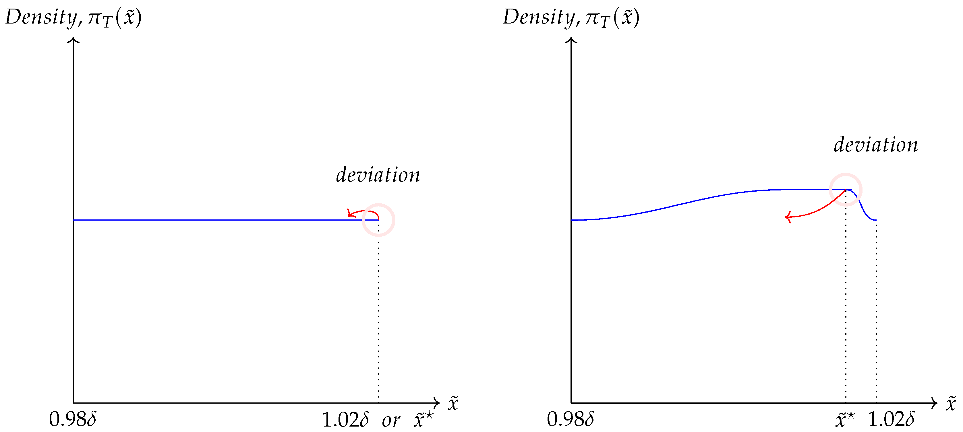
Figure 2. Two kernel density distributions.

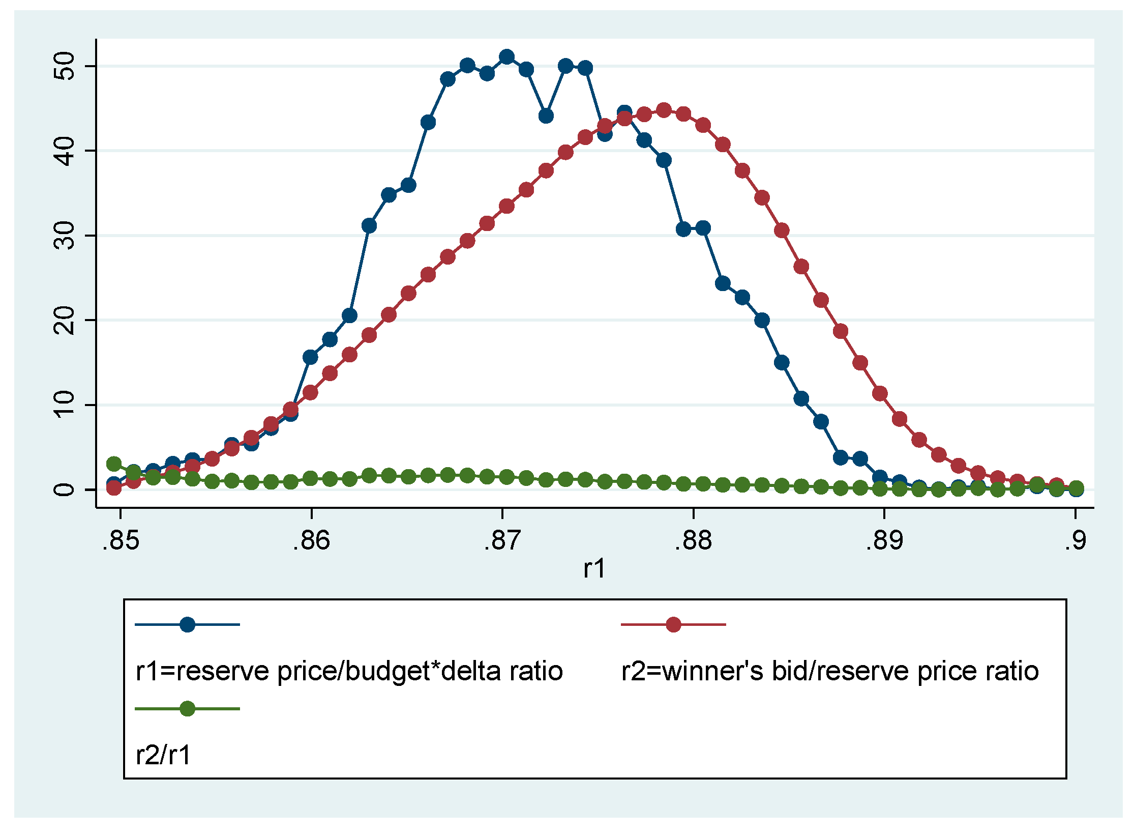
Figure 3. Multihead self-attention.

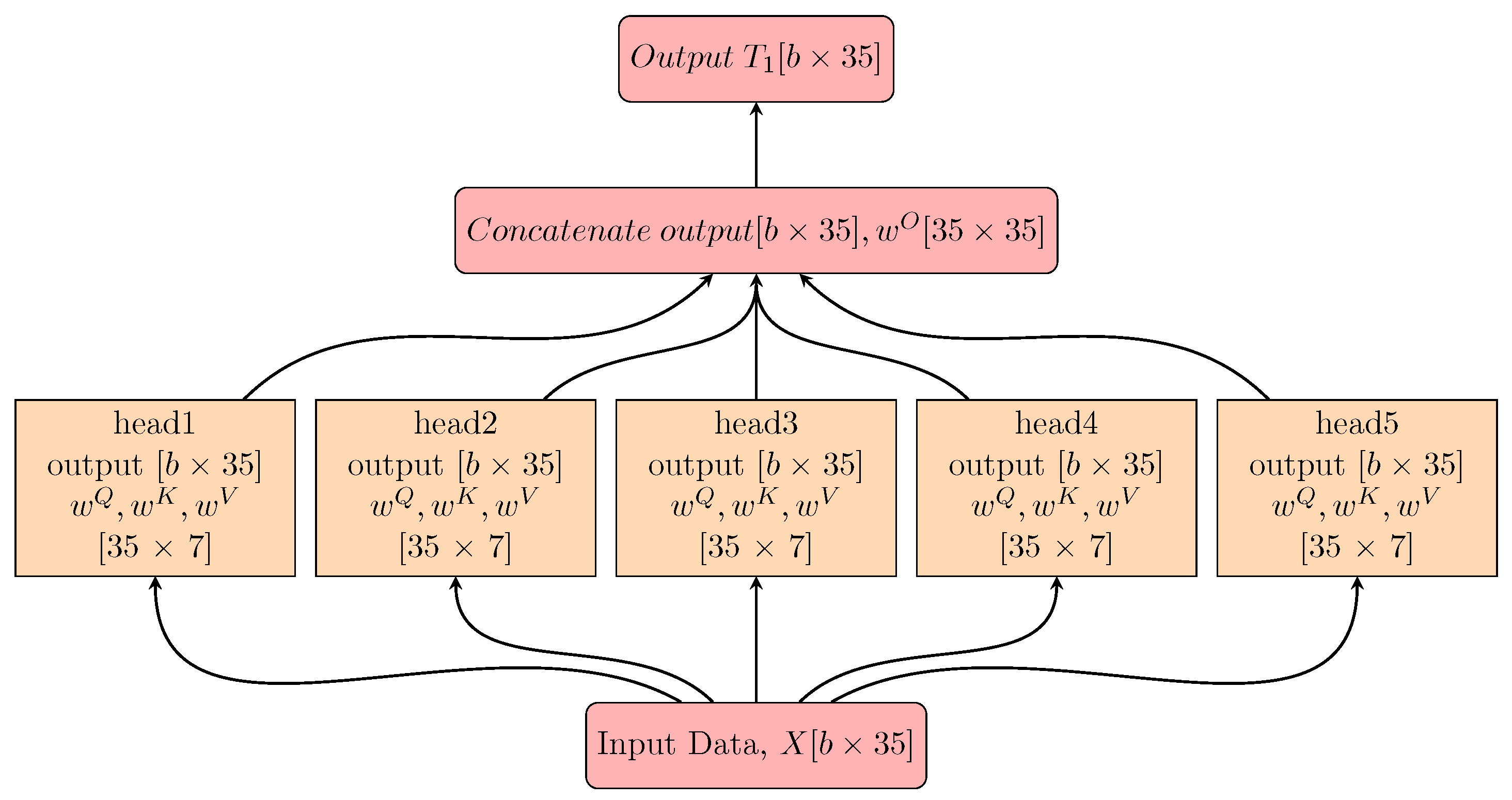
Figure 4. The first convolutional layer.

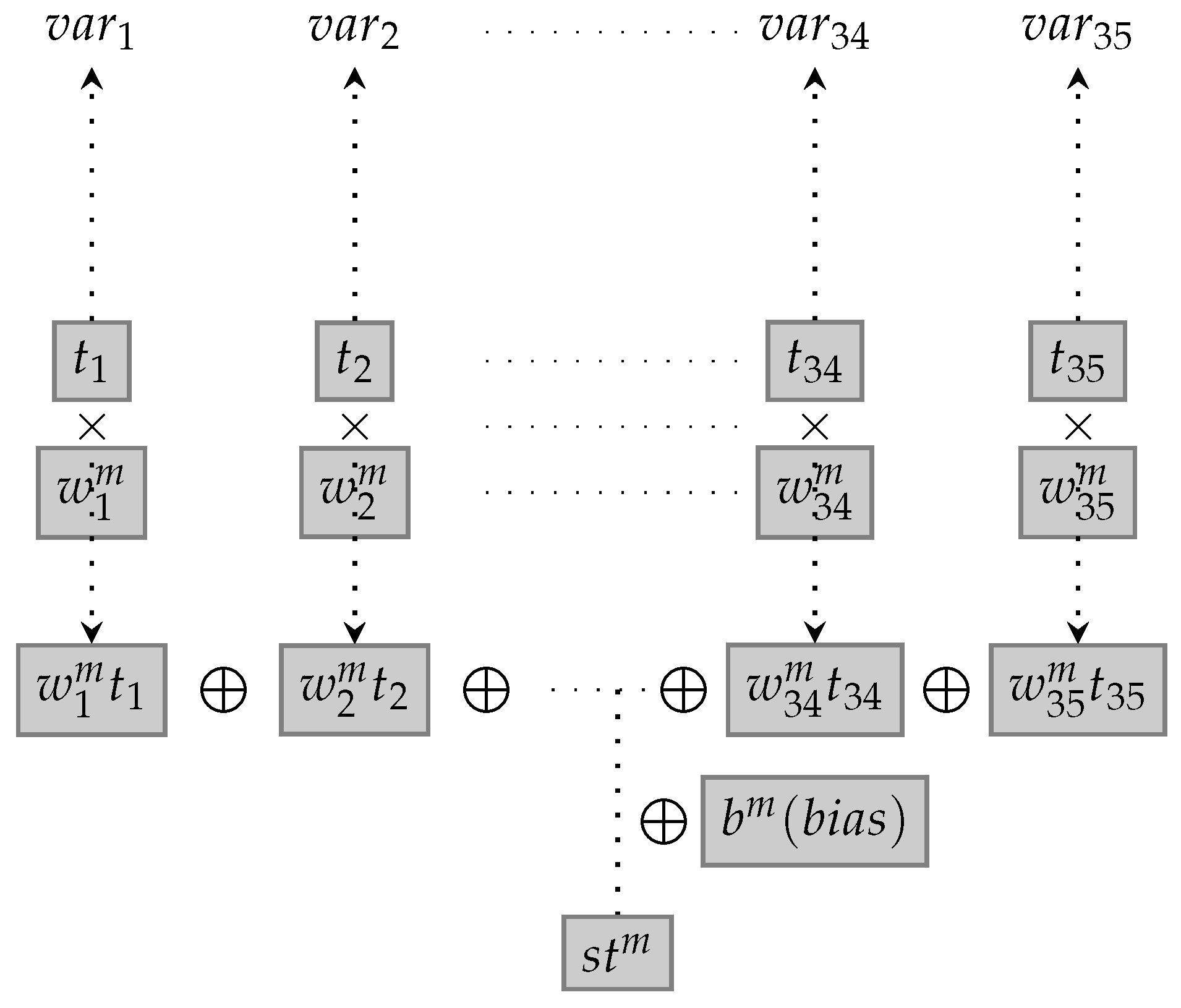
Figure 5. The second convolutional layer.

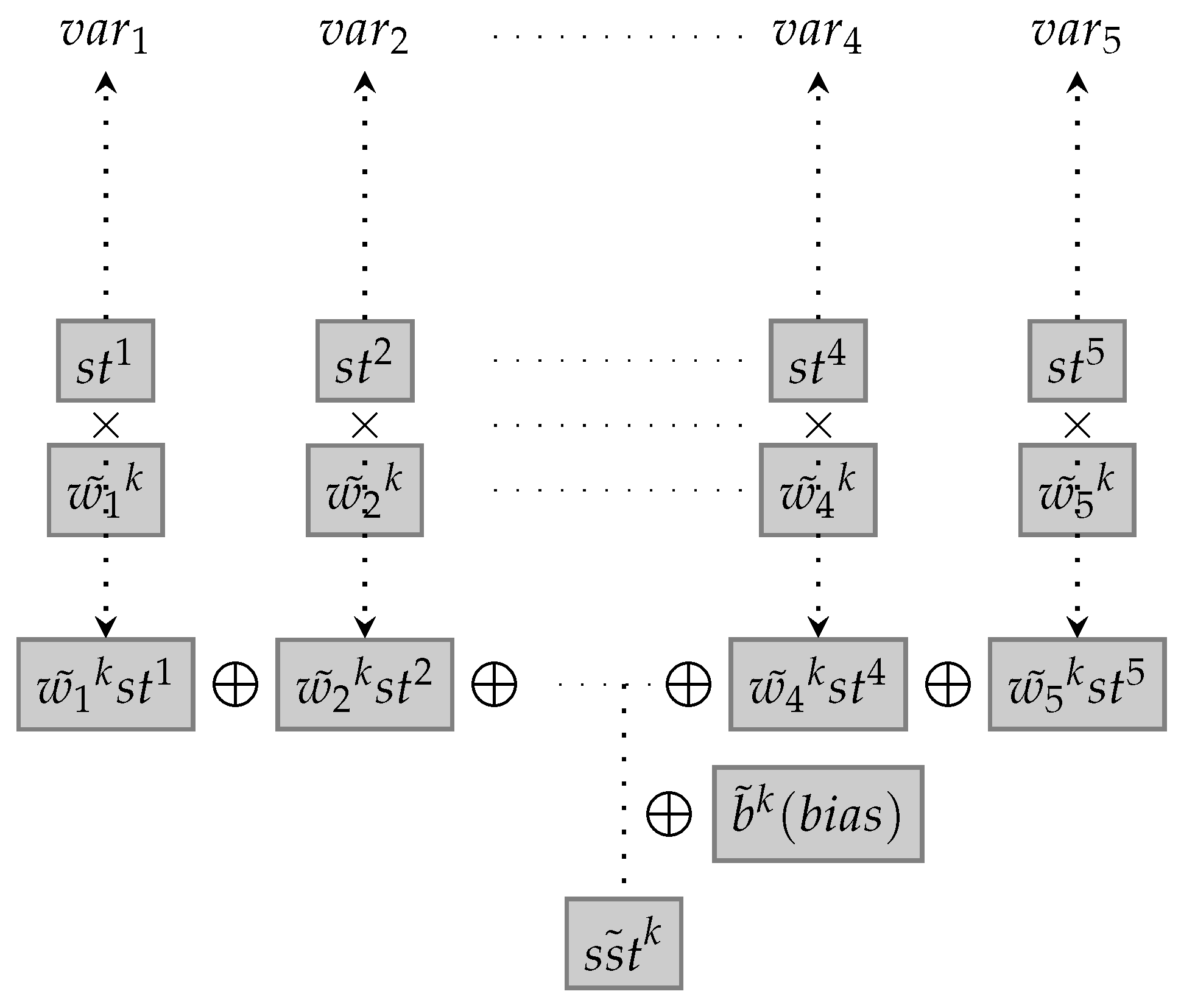
Figure 6. The distribution of predicted random cutoffs.

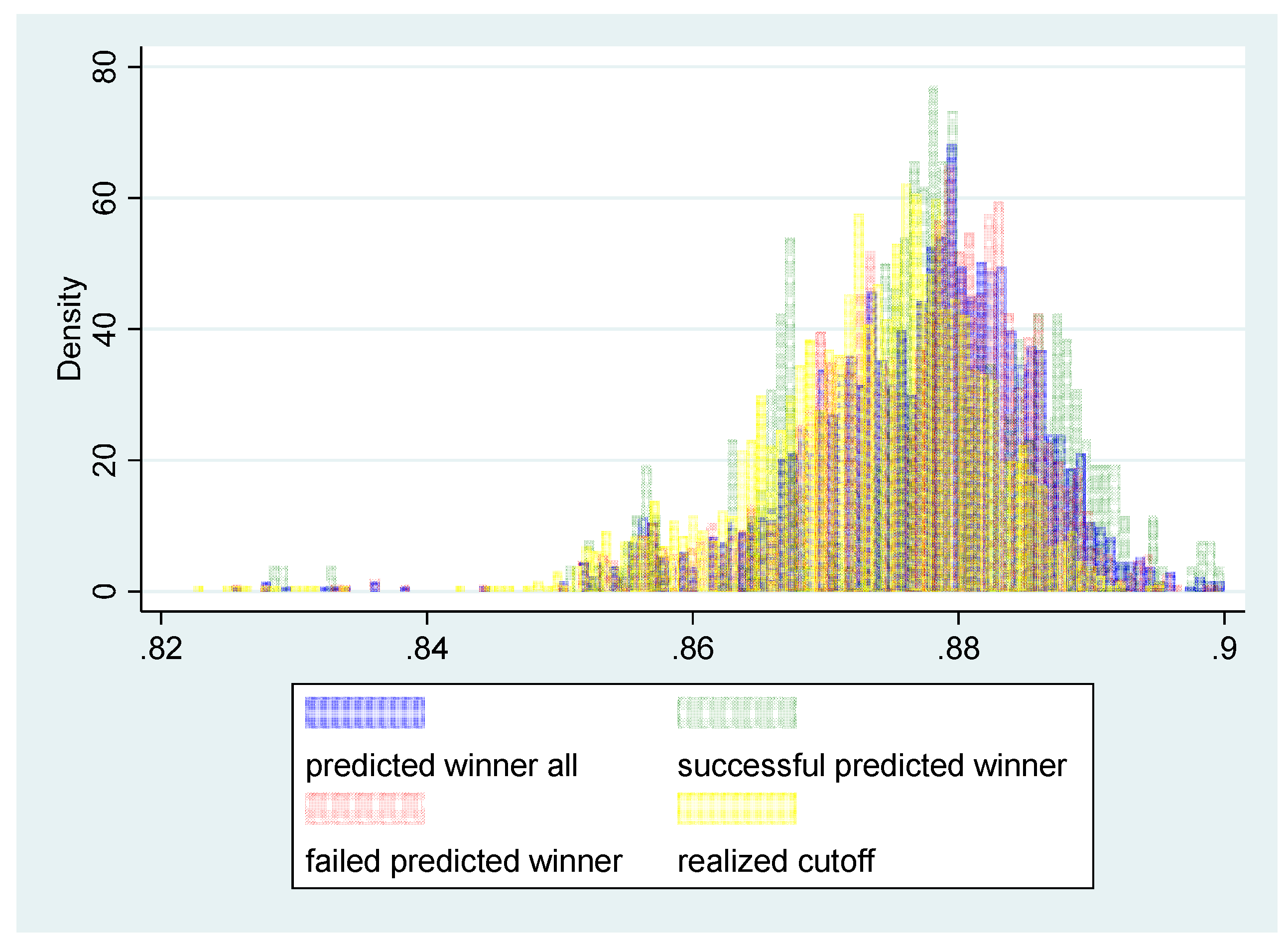
Table 1. The ratio between two kernel density distributions.

OBS	Mean	Std.Dev	Min	Max
50	0.935	0.650	0.019	3.058

Table 2. The rate of successful prediction.

	Frequency	Percent
Fail	1,422	79.75
Success	361	20.25

Disclaimer/Publisher’s Note: The statements, opinions and data contained in all publications are solely those of the individual author(s) and contributor(s) and not of MDPI and/or the editor(s). MDPI and/or the editor(s) disclaim responsibility for any injury to people or property resulting from any ideas, methods, instructions or products referred to in the content.

© 2024 by the authors. Licensee MDPI, Basel, Switzerland. This article is an open access article distributed under the terms and conditions of the Creative Commons Attribution (CC BY) license (http://creativecommons.org/licenses/by/4.0/).

Copyright: This open access article is published under a Creative Commons CC BY 4.0 license, which permit the free download, distribution, and reuse, provided that the author and preprint are cited in any reuse.

Downloads

Views

Comments

Subscription

Notify me about updates to this article or when a peer-reviewed version is published.

MDPI Initiatives

Important Links

Choose an area of interest and we will send you notifications of new preprints at your preferred frequency.

Disclaimer

Competitive Bidding Strategy in an Auction with Random Cutoff—Randomness Is Always Unpredictable?

Abstract

Keywords:

Subject:

1. Introduction

1.1. Related Literature

1.2. Purpose of this Study

2. Analysis

2.1. Detailed Bidding & Tendering Process

2.2. Investigation of Symmetric Bayes Nash Equilibrium

2.2.1. Model Description

2.2.2. Non-Existence of Symmetric Bayes Nash Equilibrium

2.3. Discussion on Competitive Bidding Strategy

3. Empirical Investigation of Bidding Strategy

3.1. Data Description

3.2. Main Model Architecture

3.2.1. Data Construction

3.2.2. Self-Attention Mechanism

3.2.3. 1D Convolution Layer

3.3. Results

4. Concluding Remarks

References

MDPI Initiatives

Important Links

Subscribe