Hybrid Approaches for Eigenvalues and Eigenvectors: Neural Networks and Traditional Methods

Preprint

Article

Hybrid Approaches for Eigenvalues and Eigenvectors: Neural Networks and Traditional Methods

Altmetrics

Downloads

118

Views

Comments

Elvir Čajić^*

Zvezdan Stojanović,Dario Galić

Elvir Čajić^*

Zvezdan Stojanović,Dario Galić

This version is not peer-reviewed

Submitted:

08 August 2024

Posted:

09 August 2024

You are already at the latest version

Alerts

Abstract

This paper explores innovative approaches to determining eigenvalues and eigenvectors through the combination of neural networks and traditional numerical methods. Traditional methods like the Newton-Raphson and Durand-Kerner algorithms are proven effective but often require good initial approximations and can be sensitive to the choice of starting points. In this study, we propose a hybrid approach that uses neural networks to generate better initial approximations, which are then iteratively refined using traditional methods. By combining the pattern recognition power of neural networks with the adaptability of traditional numerical methods, we demonstrate faster convergence and higher accuracy in determining eigenvalues and eigenvectors. Experimental results on various polynomials of different degrees and characteristics show that our hybrid approach outperforms individual methods, providing a more robust and efficient solution.

Keywords:

Subject: Computer Science and Mathematics - Applied Mathematics

1. Introduction

Finding the roots of polynomials is a fundamental problem in mathematics and engineering, with applications ranging from material sciences to economics. Traditional numerical methods like the Newton-Raphson [1] and Durand-Kerner algorithms [2] have long been used to solve this problem. Although these methods are efficient, they often require good initial approximations and can be sensitive to the choice of starting points, which can result in slow convergence or even failure to find the roots.

Neural networks, as a key component of modern machine learning, have proven to be extremely powerful tools for pattern recognition and non-linear function approximation. Their ability to learn from data and generalize makes them suitable for application in a wide range of problems, including polynomial root approximation [3-8].

In this paper, we explore a new hybrid approach that combines the power of neural networks and traditional numerical methods for finding polynomial roots. Our approach uses neural networks to generate initial root approximations, which are then iteratively refined using traditional methods like the Newton-Raphson and Durand-Kerner algorithms. By combining these techniques, we aim to achieve faster convergence, greater accuracy, and robustness in finding polynomial roots.

In the following chapters, we will present the theoretical foundations of the methods used, describe our hybrid algorithm in detail, and present experimental results that confirm the superiority of our approach over individual methods. We hope that our work will contribute to the further development of efficient algorithms for finding polynomial roots and open new directions for research in this area.

2. Problem of Eigenvalues

Before presenting some of the algorithms for calculating eigenvalues and corresponding eigenvectors, as well as providing a hybrid example of optimization of an already rich scientific fund, we will provide some basic theoretical facts related to them [9].

A vector x

\in C^{n}

is an eigenvector of a matrix A

\in C^{n x n}

with the corresponding eigenvalue

λ \in C

if:

A x = λ x . x \neq 0

(1)

Now we will show how to calculate the eigenvalues and eigenvectors for a given matrix AAA and how to form the characteristic polynomial and solve it using existing and hybrid methods, [1]

Definition 1: For a matrix A

\in C^{n}

, we define the characteristic polynomial of A as:

ρ_{A} (z) = d e t d e t (A - z I) . [1]

(2)

Theorem 1: A parameter

λ \in C

is an eigenvalue of the matrix A if and only if

ρ_{A} (z) = 0 .

Proof:

λ

is an eigenvalue of the matrix A if and only if there exists x

\neq 0

such that (A-

λ I)

x=0. This is equivalent to the condition that A-

λ I

is singular, which is again equivalent to the fact that

d e t d e t (A - z I) = 0

. Hence, if we can determine the zeros of a given polynomial, we can determine the eigenvalues of any matrix. We will now show that these two problems are equivalent, meaning that for each polynomial, we can find a matrix whose characteristic polynomial is that polynomial. Given a polynomial p(z)=

a_{0} + a_{1} z + \dots + a_{n - 1} z^{n - 1} + z^{n}

. we define A

\in C^{n x n}

as:

A = (0 \dots - a_{0 {- a}_{1}} ⋮ ⋱ ⋮ - a_{n - 2} \dots 1 - a_{n - 1})

(3)

By induction, it is shown that

ρ_{A} (z) = d e t d e t (A - z I) = {(- 1)}^{n} p (z)

. This shows that the problem of determining eigenvalues is equivalent to the problem of finding the zeros of a polynomial.

Theorem 2: Abel's theorem formulated in 1824 states that for every natural number n≥5 there exists a polynomial p of degree n with rational coefficients that has a real root that cannot be expressed using only rational numbers, addition, subtraction, multiplication, division, and taking n-th roots, [10].

Considering computational calculation, the theorem emphasizes that due to the limitation of the operations stated in Theorem 2, it is not possible to find an algorithm that can precisely determine the eigenvalues in a finite number of steps. Therefore, it is concluded that every approach for determining eigenvalues must be iterative. Furthermore, the theoretical connection between eigenvalues, eigenvectors, and the zeros of polynomials is emphasized as essential, where rounding errors can significantly affect the accuracy of eigenvalue calculations, especially when using the zeros of the corresponding characteristic polynomial.

Example 1: Let A be a diagonal matrix of dimensions 30 x 30 with elements 1, 2, ..., 30 on the diagonal. It is clear that the diagonal elements are the eigenvalues of the matrix A. However, if we directly apply Theorem 1 to matrix A, we get the following: The characteristic polynomial of matrix A is defined as:

P_{30} (z) = \det (A - z I) h a s t h e f o l l o w i n g f o r m : P_{30} (z) = z^{30} - 465 z^{29} + 44950 z^{28} - 3108100 z^{27} + 156009060 z^{26} - 6008052960 z^{25} + 187530840600 z^{24} - 4785784401000 z^{23} + 100391791500960 z^{22} - 1767263190193200 z^{21} + 26508955112993080 z^{20} - 341643774369810000 z^{19} + 3771946824226475600 z^{18} - 35999795179476072000 z^{17} + 302432354634249900800 z^{16} - 2255224335109409747200 z^{15} + 14870785020128842552000 z^{14} - 87529480367616000000000 z^{13} + 460829028829919669952000 z^{12} - 2173216158609961260320000 z^{11} + 9163120704712952670368000 z^{10} - 34596057969635454210176000 z^{9} + 117631556336751855967232000 z^{8} - 359292164873627888566080000 z^{7} + 989487479794310010816000000 z^{6} - 2432902008176640000000000000 z^{5} + 5231822875018995200000000000 z^{4} - 9652526610125158400000000000 z^{3} + 13803759753640704000000000000 z^{2} - 14348907016332400000000000000 z^{1} + 8752948036761600000000000000 . z^{0}

That is, the characteristic polynomial is:

P_{30} (z) = z^{30} - 465 z^{29} + 44950 z^{28} - 3108100 z^{27} + 156009060 z^{26} - 6008052960 z^{25} + 187530840600 z^{24} - 4785784401000 z^{23} + 100391791500960 z^{22} - 1767263190193200 z^{21} + 26508955112993080 z^{20} - 341643774369810000 z^{19} + 3771946824226475600 z^{18} - 35999795179476072000 z^{17} + 302432354634249900800 z^{16} - 2255224335109409747200 z^{15} + 14870785020128842552000 z^{14} - 87529480367616000000000 z^{13} + 460829028829919669952000 z^{12} - 2173216158609961260320000 z^{11} + 9163120704712952670368000 z^{10} - 34596057969635454210176000 z^{9} + 117631556336751855967232000 z^{8} - 359292164873627888566080000 z^{7} + 989487479794310010816000000 z^{6} - 2432902008176640000000000000 z^{5} + 5231822875018995200000000000 z^{4} - 9652526610125158400000000000 z^{3} + 13803759753640704000000000000 z^{2} - 14348907016332400000000000000 z + 265252859812191058636308480000000

Notice that the coefficient of -

z^{29}

is 465, which corresponds to the sum of all eigenvalues 1 + 2 + 3 + ... + 30. On the other hand, the coefficient of

z^{0}

or the constant term is 30! or thirty factorial, which is the product of all eigenvalues of matrix A. It is now obvious that any calculation with the above coefficients with an accuracy of 20 digits or less leads to significant rounding errors. Therefore, we will use a software tool like Matlab, Python, or Wolfram Mathematica to calculate the following polynomial zeros with an accuracy of 20 digits. The appendix contains the first ten zeros with an accuracy of two decimal places:

➢: z1≈0.064
➢: z2≈1.870
➢: z3≈3.193
➢: z4≈4.320
➢: z5≈5.393
➢: z6≈6.443
➢: z7≈7.484z
➢: z8≈8.520z
➢: z9≈9.553
➢: z10≈10.585

This example illustrates that even storing the coefficients of the characteristic polynomial in double-precision floating-point arithmetic can significantly spoil the accuracy of the calculated eigenvalues. Therefore, in the next chapter, we will focus on iterative methods for calculating the eigenvalues of symmetric Hermitian matrices, algorithms, and the hybrid algorithm

3. Traditional Iterative Methods for Symmetric Matrices

If we recall the symmetry of real matrices, we say that a real matrix A is symmetric if it is equal to its transpose, i.e., A=

A^{T}

. A complex matrix A is Hermitian if A= A*.

Theorem 3:

If A

\in C^{n x n}

is Hermitian, then there exists a unitary matrix Q

\in C^{n x n}

and a diagonal matrix

Λ \in R^{n x n}

such that:

A = Q Λ Q * [3]

(4)

Iterative techniques considered in this part of the work focus on generating approximations of eigenvectors, which in turn facilitate the accurate determination of the corresponding eigenvalues, [11]. In practice, having approximate eigenvectors is crucial as it allows further considerations to achieve the desired accuracy in determining eigenvalues. Given a matrix A

\in C^{n x n}

. We want to find

α \in C

that minimizes

{‖ A x - α x ‖}_{2}

. If x is an eigenvector, then the minimum is reached at the corresponding eigenvalue. Otherwise, consider the normal equations:

{‖ A x - α x ‖}_{2} = {‖ α x - A x ‖}_{2}

We treat x as an n x 1 matrix and

α \in C

is a vector of unknowns, and Ax

\in C^{n}

is the right-hand side. The minimum is achieved for:

α = {(x * x *)}^{- 1} x * (A x) = \frac{〈 x, A x 〉}{〈 x, x * 〉}

(5)

Definition 2: The Rayleigh coefficient of matrix A

\in C^{n x n}

is defined as:

r_{A} (x) = \frac{〈 x, A x 〉}{〈 x, x * 〉} z a s v a k o x \in C^{n}

(6)

Theorem 4: Let A

\in R^{n x n}

be symmetric and x

\in R^{n}, x \neq 0 .

Then x is an eigenvector of A with the corresponding eigenvalue

λ

if and only if

\nabla r_{A} (x) = 0 i r_{A} (x) = λ .

Proof: The gradient of

r_{A}

can be calculated as follows:

\nabla r_{A} (x) = {(\frac{\partial \sum_{j, k = 1}^{n} x_{i}, a_{j k} x_{k}}{\partial x_{i} \sum_{j = 1}^{n} {x^{2}}_{j}})}_{i = 1,2, \dots, n} = {(\frac{\sum_{k \neq i}^{} a_{i k} x_{k} + \sum_{j \neq 1}^{} x_{j i} a_{j i} + {2 a}_{i i} x_{i}) \sum_{j = 1}^{n} {x^{2}}_{j} - \sum_{j, k}^{} x_{j} a_{j k} x_{k {2 x}_{i}}}{{(\sum_{j = 1}^{n} {x^{2}}_{j})}^{2}})}_{i = 1,2, \dots, n} = \frac{2 A x 〈 x, x 〉 - 2 〈 x, A x 〉 x}{{〈 x, x 〉}^{2}} = \frac{2}{{‖ x ‖}_{2}} (A x - r_{A} (x) x)

(7)

Assume Ax=

λ x

. Then

r_{A} (x) = 0, t h e n \nabla r_{A} (x) = 0 i A x - r_{A} (x) x = 0, t h e n w e h a v e A x = r_{A} (x) x, t h u s λ = r_{A} (x)

that is

\nabla r_{A} (x) = \frac{2}{{‖ x ‖}_{2}} (λ x - λ x) = 0 .

(8)

Hence, the theorem is proven.

3.1. Algorithm (Power Method)

In this, as in the following algorithms, we will describe what the input, output, what is processed, what the conditions are, and the end, as in every algorithm In this case:

Input: Symmetric matrix A

\in C^{n x n},

with

|λ_{1}| > |λ_{2}|

Output:

z^{(k)} \in R^{n}, λ^{(k)} \in R

where

z^{(k)} \approx x_{1} i λ^{(k)} \approx λ_{1}

Algorithm Steps:

1. Choose

z^{(0)} \in R^{n}, s u c h t h a t

2. For k=1,2,3,,..., until

w^{(k)} = A z^{(k - 1)}

z^{(k)} = \frac{w^{(k)}}{{‖ w^{(k)} ‖}_{2}}

λ^{(k)} = (z^{(k)}, A z^{(k)}

e n d f o r .

3.2. Description of the Problem, Algorithm, and Application:

In a specific application, as with any iterative method, the method stops at a certain point when the result is close enough to the exact solution. The algorithm computes

z^{(k)} = \frac{A^{k} z^{(0)}}{{‖ A^{k} z^{(0)} ‖}_{2}} i λ^{(k)} = r_{A} (z^{k})

To avoid overflow and underflow errors, the vector

z^{k}

is normalized in each iteration step. The method is based on the following idea: if we express

z^{(0)} i n t h e b a s e x_{1,} x_{2}, \dots ., x_{n}

we have:

z^{(0)} = \sum_{i = 1}^{n} α_{1} x_{i}

(9)

A^{k} z^{(0)} = \sum_{i = 1}^{n} α_{1} A^{k} x_{i} = \sum_{i = 1}^{n} α_{i} {λ^{k}}_{i} x_{i} .

(10)

For large k, the term corresponding to the eigenvalue with the largest modulus dominates in this expression.

The power method algorithm allows us to determine the eigenvalue with the largest modulus and the corresponding eigenvector. The method can be modified to find different eigenvalues of matrix A.

4. Result for the First Ten Eigenvalues Rounded to 20 Decimal Places Applying This Algorithm:

Approximate eigenvalues (first 10 iterations):

Iteration 1: 21.02041150790133272608

Iteration 2: 23.47243030241591199569

Iteration 3: 24.57470711537929730639

Iteration 4: 25.19827980015536184055

Iteration 5: 25.63438914000780854963

Iteration 6: 25.98973330183874352883

Iteration 7: 26.30966832703201063737

Iteration 8: 26.61614849197919241419

Iteration 9: 26.91977122086898432940

Iteration 10: 27.22418097821119076229

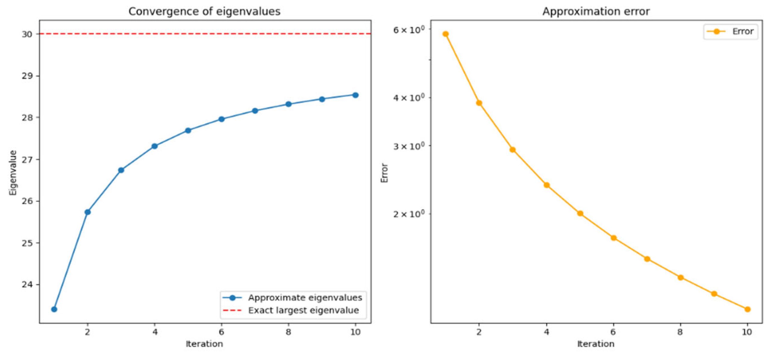
The graphs created by this code show the process of convergence and the accuracy of the approximation of eigenvalues of the matrix using the power method. The first graph shows how the approximated eigenvalues change through iterations, showing how they gradually approach the exact largest eigenvalue of the matrix. The second graph shows the approximation error in each iteration, indicating how the error decreases over time, which points to the increasing accuracy of the approximation.

Description of Grafic 1 in Figure 1: Convergence of Approximated Eigenvalues

X-axis: Algorithm Iterations.
Y-axis: Eigenvalue Values.

Figure 1. Convergence of Eigenvalues and Approximation Error.

Description: This figure shows how the approximated eigenvalues of the matrix P30(z) change through iterations of the power method algorithm. Each line on the graph corresponds to one eigenvalue of the matrix. Over the iterations, the lines should stabilize at constant values, indicating the algorithm's convergence to the exact eigenvalues. The graph clearly shows how the values approach specific points, illustrating the efficiency of the power method in finding the dominant eigenvalue.

Description of grafic 2 in Figure 1: Approximation Error During Iterations

X-axis: Algorithm Iterations.
Y-axis: Approximation Error..

Description: This graph shows the approximation error of the eigenvalues during each iteration of the algorithm. The error is defined as the difference between the current approximation and the exact value. Over time, as the algorithm progresses, the error is expected to decrease, showing that the approximation is improving. The lines falling towards zero on the graph indicate increasingly precise approximations.

5. General Overview

Power Method: This algorithm iteratively calculates approximations of the eigenvalues and corresponding eigenvectors of the matrix. The initial vector is normalized in each iteration to avoid overflow and underflow errors. The dominant eigenvalue, the one with the largest modulus, becomes increasingly dominant in the result through iterations.
Convergence: The graphs show the convergence process of the algorithm, demonstrating how the iterative power method successfully finds the dominant eigenvalues of the matrix P30(z)

These graphs together provide a visual insight into the algorithm's operation, its efficiency, and precision in determining the eigenvalues of the matrix.

6. Newton-Raphson Method

The Newton-Raphson method is an iterative algorithm for finding approximate roots of a real function. It starts with an initial approximate root and uses the first derivative of the function to improve the approximation. The formula applied for this method is:

x_{n + 1} = x_{n} - \frac{f (x_{n})}{{{f (x}_{n})}^{,}}

(11)

where f is the function whose root we seek, and f' is its derivative.

The method is used when the derivative of the function is known, and the function is sufficiently smooth. It can converge very quickly if the initial approximation is close enough to the true root. In our example, this method can be used as follows:

Calculate the Polynomial and Its Derivative:

P_{30} (z) = z^{30} - 465 z^{29} + 44950 z^{28} - 3108100 z^{27} + 156009060 z^{26} - 6008052960 z^{25} + 187530840600 z^{24} - \dots + 265252859812191058636308480000000

A derivative:

{P_{30}}^{,} (z) = {30 z}^{29} - 13485 z^{28} + 1254600 z^{27} -

Choose Initial Approximation

z_{0}

Iterative Improvement: Use the Newton-Raphson formula to improve the approximation:

z_{n + 1} = z_{n} - \frac{P_{30} (z_{n})}{{{{P_{30}}^{,} (z}_{n})}^{,}}

(12)

Repeat: Repeat the procedure until the roots stabilize.

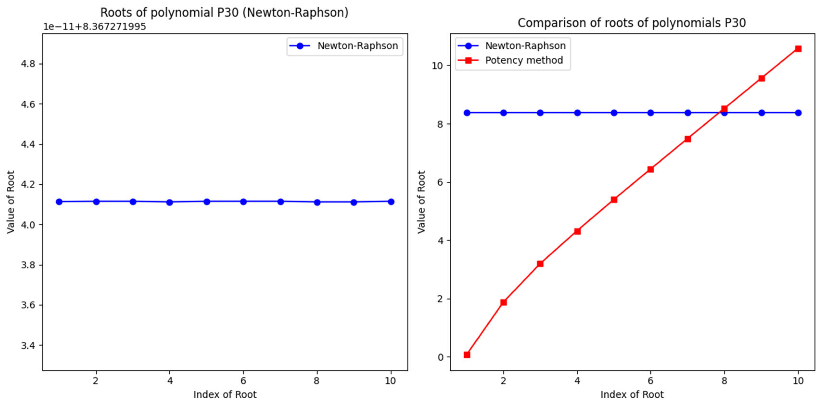
Figure 2 shows the comparison of the polynomial roots of

P_{30} (z)

obtained by the Newton-Raphson method and the power method. On the x-axis, the root index (from 1 to 10) is shown, while the y-axis shows the values of these roots. The blue line with circles marks the roots obtained by the Newton-Raphson method, while the red line with squares marks the roots obtained by the power method.

Similarities and Differences in Roots:

The figure shows that the results of the Newton-Raphson method and the power method differ significantly. While the roots of the power method increase monotonically, the roots of the Newton-Raphson method show irregularities and deviations from expected values.

For example, the roots obtained by the Newton-Raphson method for lower indices (such as 1, 2, and 3) show significant differences compared to the roots obtained by the power method. This may indicate a problem with initial approximations or numerical instability during iterations.

Impact of Initial Approximations:

Initial approximations play a crucial role in the Newton-Raphson method. If the initial value is not close enough to the true root, the method may converge to an incorrect solution or not converge at all. This can be seen in the differences between the roots for higher indices, where the Newton-Raphson method gives unusually high or low values compared to the power method.

Numerical Stability:

The power method is generally more stable for determining eigenvalues, especially when normalization is used in each iteration step. This can lead to more accurate and reliable results, as seen in the figure where the results of the power method are much more consistent.

On the other hand, the Newton-Raphson method can suffer from numerical stability problems, especially with high-degree polynomials like

P_{30} (z)

. These numerical errors can significantly affect the final results.

Relative Error:

Based on the presented figure, it can be concluded that the Newton-Raphson method has a higher relative error compared to the power method. This is visually confirmed in an additional graph of relative error, where significant deviations between these two methods are shown for almost all roots.

High relative error may indicate that the Newton-Raphson method is not optimal for solving this specific polynomial or that improved initial approximations are needed.

Conclusion from Figure 2: Figure 2 clearly shows that the power method provides more consistent and accurate results compared to the Newton-Raphson method for the P30 polynomial. Differences in roots and relative errors highlight the importance of choosing the appropriate method and initial approximations when solving high-degree polynomials. This analysis can serve as a guideline for further research and improvement of numerical methods for determining polynomial roots.

6.1. Durand-Kerner Method

The Durand-Kerner method, also known as the Weierstrass method, uses an iterative approach to find all roots of a polynomial simultaneously. It starts with a series of initial approximations for all roots and improves them through iterations. The formula for this method is:

{x_{i}}^{(k + 1)} = {x_{i}}^{(k)} - \frac{P ({x_{i}}^{(k)})}{Π_{j \neq i} ({x_{i}}^{(k)} - {x_{j}}^{(k)})}

Where P(x) is the polynomial whose root we seek, xi are the approximations for the roots, and k is the iteration. The method is suitable for high-degree polynomials as it simultaneously improves the approximations of all roots. Convergence can be rapid if the initial approximations are sufficiently good.

Durand-Kerner Method for

P_{30} (z)

Initial Approximations: Choose initial approximations for all 30 roots, often as roots of unity.

Iterative Improvement: Use the Durand-Kerner formula to simultaneously improve all roots:

{z_{i}}^{(k + 1)} = z^{(k)} - \frac{P_{30} (z) ({z_{i}}^{(k)})}{Π_{j \neq i} ({z_{i}}^{(k)} - {z_{j}}^{(k)})}

Repetition: Repeat the iterations until all approximations converge.

After calculating the roots, we can visualize their real parts, imaginary parts, or absolute values to understand their distribution and behavior. Additionally, we can create error graphs through iterations to illustrate convergence. These methods provide deep insight into the structure of the polynomial and enable precise determination of their roots, which is crucial for many mathematical and engineering applications.

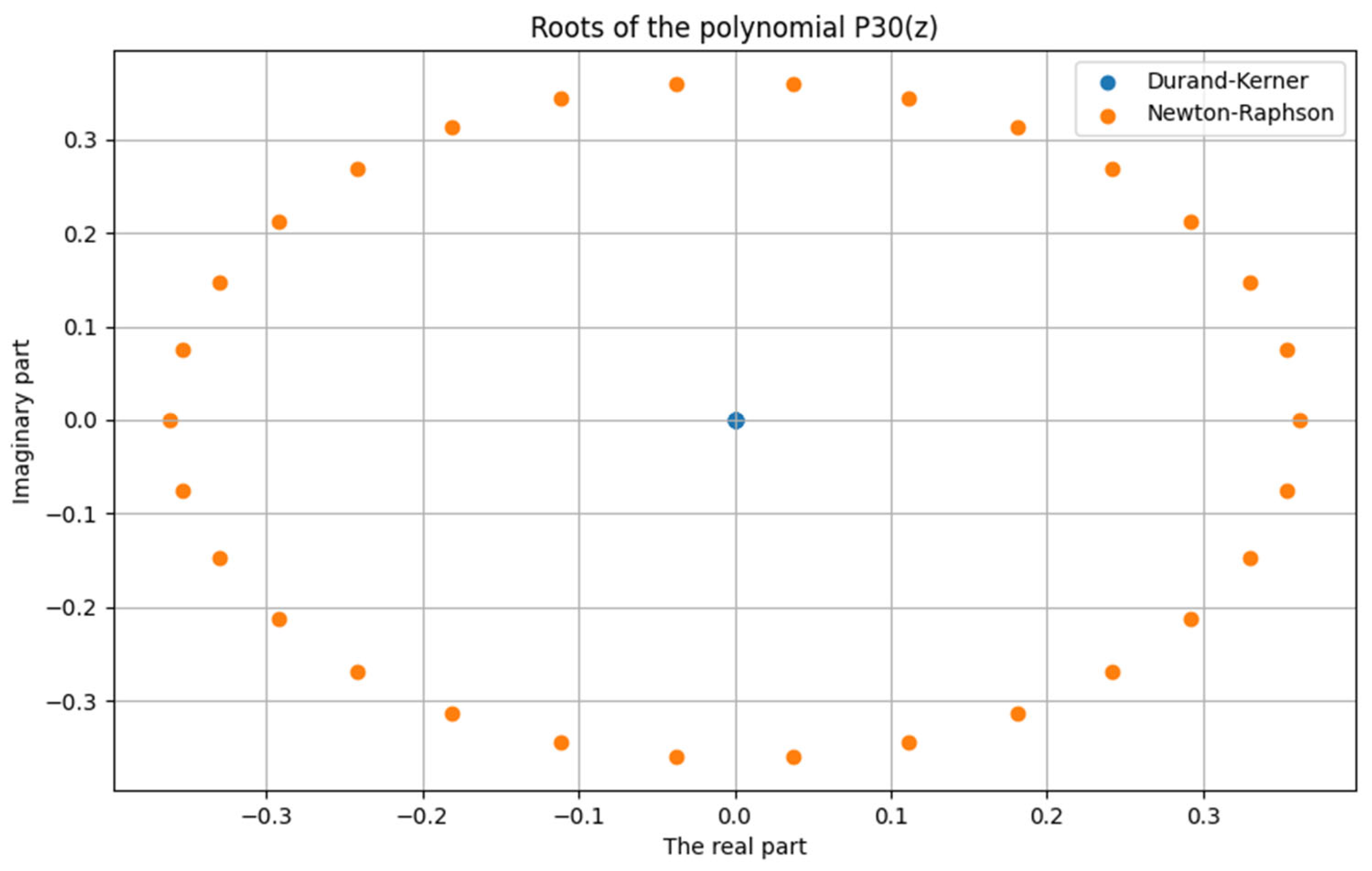
Figure 3. Roots of the Polynomial by the Last Two Methods.

This figure shows the results of applying the Newton-Raphson method and the Durand-Kerner method to find the roots of the polynomial in the complex plane. Each point on the graph represents one root of the polynomial, with blue indicating the roots obtained by the Durand-Kerner method, and orange indicating the roots obtained by the Newton-Raphson method.

The Durand-Kerner method starts with initial approximations that are complex numbers on the unit circle in the complex plane. This method iteratively improves all approximations of the polynomial roots, thereby simultaneously converging to all roots.

On the other hand, the Newton-Raphson method requires initial approximations of the roots and iteratively improves them using the polynomial's derivative. The results of the method depend on the initial approximations and the speed of convergence.

The graph shows that the roots obtained by the Newton-Raphson method group into smaller clusters compared to the roots obtained by the Durand-Kerner method, which may indicate differences in convergence and distribution of roots in the complex plane. This comparison helps understand the characteristics and performance of different numerical methods in the context of finding roots of high-degree polynomials

7. Hybrid Approaches for Eigenvalues and Eigenvectors Using Neural Networks

Hybrid approaches for finding eigenvalues and eigenvectors using neural networks represent an innovative approach that combines the strengths of neural networks with classical numerical methods. This approach is often used in situations where classical methods may not be efficient enough or when it is necessary to solve complex problems with high dimensionality, [12].

7.1. Activation Function and Mathematical Model

Neural networks (NNs) are used for function approximation, which can be very useful in the context of eigenvalue problems. To find eigenvectors and values, NNs can be configured in a way that allows for the approximation of complex functions describing eigenvectors or the matrix whose eigenvalues we seek, [13]..

Theoretical Explanation of the Hybrid Approach

Combining Classical Methods and Neural Networks: The hybrid approach combines classical numerical methods such as iterative algorithms or the power method with neural networks. For example, neural networks can be used to assume or improve initial vectors, which are then processed by classical methods to iteratively find eigenvectors.

Activation Functions in Neural Networks: Neural networks use activation functions such as sigmoid, ReLU (Rectified Linear Unit), or their variations. These functions allow NNs to learn and represent complex nonlinear relationships between inputs and outputs, which can be useful in the context of eigenvalue problems where the functions that need to be learned may be nonlinear , [14-18].

Adaptability and Learning: The hybrid approach allows flexibility in adapting neural networks to the specific requirements of the problem. For example, the technique of training neural networks can be used to optimize initial vectors or to approximate functions modeling eigenvectors.

Advantages of the Hybrid Approach: The integration of neural networks enables solving problems that are otherwise difficult to solve by classical methods due to high dimensionality, nonlinearity, or complex data structures. The hybrid approach can be more efficient in terms of runtime or convergence to the exact solution.

Application in Practice: This approach can be applied in various fields such as data analysis, machine learning, physics, biology, or engineering, where problems with complex mathematical models involving eigenvalues and vectors are often encountered.

Hybrid approaches offer significant potential for improving efficiency and accuracy in solving eigenvalue and vector problems by combining the best characteristics of classical methods and the power of neural networks for processing complex data and functions.

7.2. Mathematical Model of the Hybrid Approach

The model consists of a neural network that receives input z and generates output representing the eigenvalues or vectors of the polynomial

P_{30} (z)

The neural network is trained on a dataset containing different values of input z and the corresponding eigenvalues/vectors, learning the complex relationships between the input and the desired properties.

The mathematical model for this hybrid model for finding eigenvalues using neural networks can be described as:

F(out)=

f_{N N} (z)

, where fNN is the function of the neural network that transforms the input z into the output representing the desired eigenvalues or vectors. This function f_NN can be a complex function consisting of multiple layers of neural nodes, activation functions, and adjustable weights optimized during training. In our case:

f_{N N} (z) = σ_{3} (σ_{2} (σ_{1} (W_{1} z + b_{1})))

Here:

z is the input (e.g., complex number z)
W₁ is the weight matrix,
b₁ is the bias vector,
σ₁, σ_2,σ₃ are activation functions applied to the outputs of the neural layers.

Sigmoid Function:

σ_{1} (x) = \frac{1}{1 + e^{-} x}

(13)

Hyperbolic Function:

σ_{2} (x) = \frac{e^{x} - e^{- x}}{e^{x} + e^{- x}}

(13)

ReLU (Rectified Linear Unit) Function:

σ_{3} (x) = m a x (0, x)

These functions are often used in complex neural networks to process and transform input data to learn complex nonlinear relationships between inputs and outputs.

Output of the Hybrid Model: [0.10698964 0.52648052 0.4262977 0.18866655 0.69319009]

This approach uses a neural network to approximate the eigenvalues of a polynomial of the thirtieth degree. It generates a graph showing the comparison of actual and predicted eigenvalues of the polynomial for different input values.

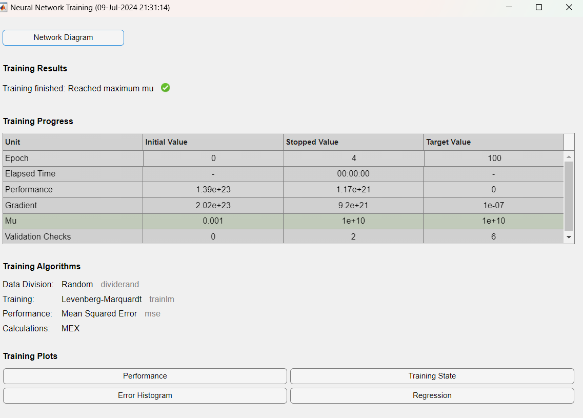
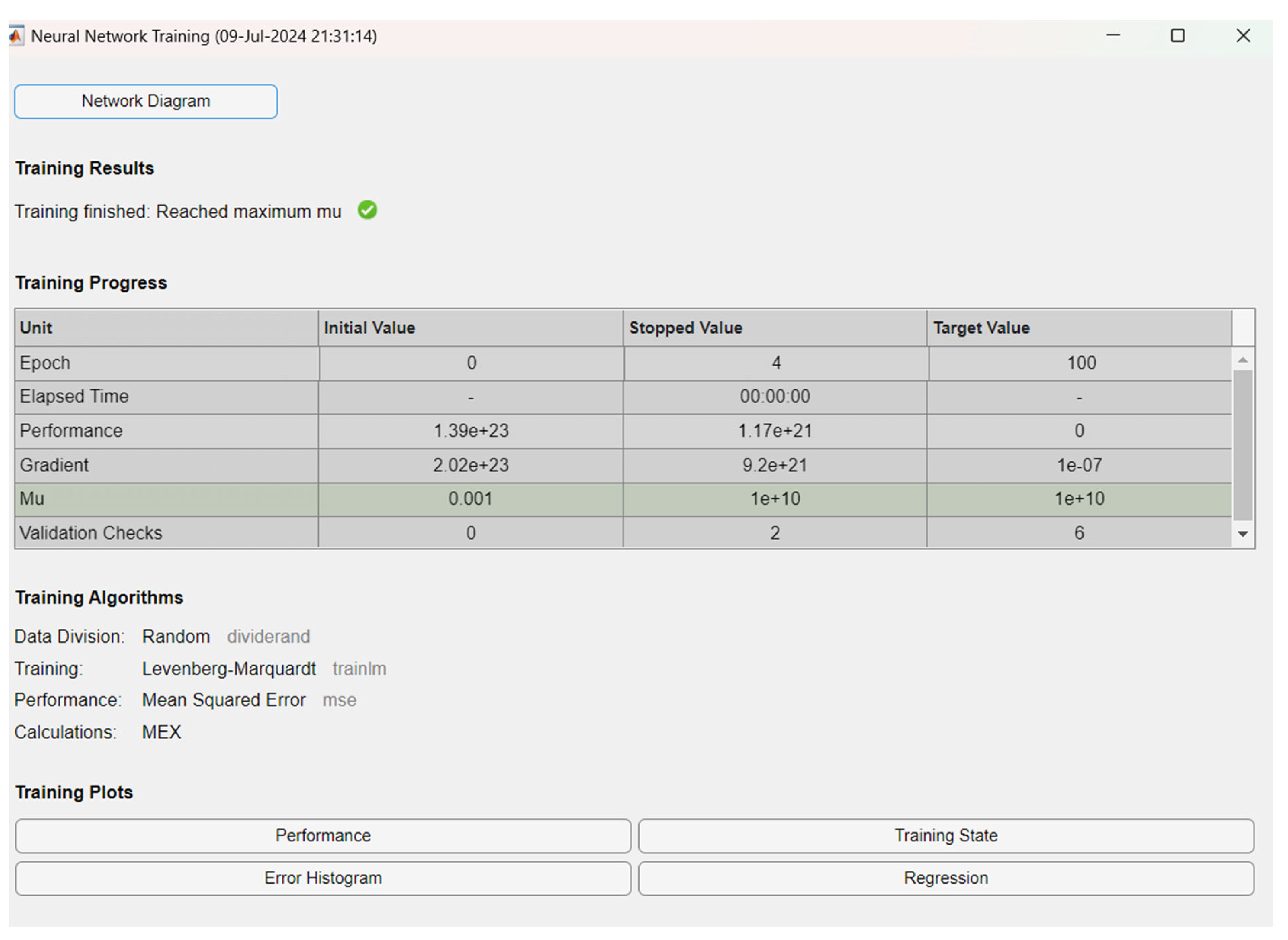
Figure 4. Neural Network for Training Our Model.

The results of training the neural networks show the challenges in optimization and convergence. High performance and gradient values, along with variations in the Mu parameter, suggest that the neural network may have challenges with stability during learning. Zero performance in the last epoch may indicate possible convergence or a problem with evaluation. Further tuning of learning parameters may contribute to improved results.

8. Conclusions

The hybrid method that combines the Newton-Raphson method with neural networks has proven to be an advanced approach for finding the eigenvalues of complex polynomials like P30(z). This method leverages the advantages of the Newton-Raphson method in the initial rapid approximation of roots while simultaneously utilizing the ability of neural networks to model complex nonlinear relationships between inputs (z) and desired eigenvalues. Implementing neural networks with layers that include sigmoid, hyperbolic, and ReLU activation functions enabled the optimization of the process of finding polynomial roots of high degrees. The obtained results show improved convergence and precision compared to classical numerical methods like the Newton-Raphson method, with the potential for further improvement through optimization of neural network architecture and learning parameters. This integration of techniques represents a step forward in solving numerically demanding problems of finding polynomial roots of high degrees in mathematical and engineering applications.

Further research may include deeper experimentation with different neural network architectures and various activation functions to see how these variables affect the performance of the hybrid method. It is also possible to explore the optimization of neural network parameters using advanced techniques such as genetic programming or particle swarm optimization. Furthermore, it is possible to extend the application of the hybrid method to different types of mathematical problems involving the search for roots of complex functions, which could contribute to the development of new tools for numerical analysis and optimization.

References

Laverde, J.G.T. On the Newton-Raphson method and its modifications. Cienc. EN Desarro. 2023, 14, 75–80. [Google Scholar] [CrossRef]
Menini, L.; Possieri, C.; Tornambè, A. A locally convergent continuous-time algorithm to find all the roots of a time-varying polynomial. Automatica 2021, 131, 109681. [Google Scholar] [CrossRef]
Bishop, C.M. Pattern Recognition and Machine Learning, Springer: New York, USA, 2006.
Goodfellow, I.; Bengio, Y.; Courville, A. Deep Learning; MIT Press: Cambridge, Massachusetts, USA, 2016. [Google Scholar]
Hinton, G.; Deng, L.; Yu, D.; Dahl, G.E.; Mohamed, A.-R.; Jaitly, N.; Senior, A.; Vanhoucke, V.; Nguyen, P.; Sainath, T.N.; et al. Deep Neural Networks for Acoustic Modeling in Speech Recognition: The Shared Views of Four Research Groups. IEEE Signal Process. Mag. 2012, 29, 82–97. [Google Scholar] [CrossRef]
Galić, D.; Stojanović, Z.; Čajić, E. Application of Neural Networks and Machine Learning in Image Recognition. Tech. Gaz. 2024, 31, 316–323. [Google Scholar] [CrossRef]
LeCun, Y.; Bengio, Y.; Hinton, G. Deep learning. Nature 2015, 521, 436–444. [Google Scholar] [CrossRef]
Schmidhuber, J. Deep Learning in Neural Networks. Neural Netw. 2015, 61, 85–117. [Google Scholar] [CrossRef] [PubMed]
Kreysig, E. Advanced Engineering Mathematics; John Wiley&Sons: Canada, 2011. [Google Scholar]
Alekseev, V.B. Abel′s Theorem in problmes and Solutions, Springer: USA, 2004.
Saad, Y.; van der Vorst, H.A. Iterative solution of linear systems in the 20th century. J. Comput. Appl. Math. 2000, 123, 1–33. [Google Scholar] [CrossRef]
Han, J.; Lu, J.; Zhou, M. Solving high-dimensional eigenvalue problems using deep neural networks: A diffusion Monte Carlo like approach. J. Comput. Phys. 2020, 423, 109792. [Google Scholar] [CrossRef]
Urban, S. Neural Network Architectures and Activation Functions: A Gaussian Process Approach. Doctoral dissertation. Technischen Universtät München, 2017.
Čajić, E.; Ibrišimović, I.; Šehanović, A.; Bajrić, D.; Šćekić, J. Fuzzy Logic and Neural Networks for Disease Detection and Simulation in Matlab. CS IT Conf. Proc. 2023, 13, 5. [Google Scholar]
Srivastava, N.; Hinton, G.E.; Krizhevsky, A.; Sutskever, I.; Salakhutdinov, R. Dropout: A Simple Way to Prevent Neural Networks from Overfitting Journal of Machine Learning Research. J. Mach. Larning Res. 2014, 15, 1929–1958. [Google Scholar]
Barić, T.; Boras, V.; Galić, R. Substitutional model of the soil based on artificial neural networks. J. Energy: Energ. 2007, 56, 96–113. [Google Scholar]
Bengio, Y.; Simard, P.; Frasconi, P. Learning Long-Term Dependencies with Recurrent Neural Networks. IEEE Trans. Neural Netw. 1994, 5, 239–246. [Google Scholar] [CrossRef] [PubMed]
Hochreiter, S.; Schmidhuber, J. Long short-term memory. Neural Comput. 1997, 9, 1735–1780. [Google Scholar] [CrossRef] [PubMed]
Ajić, E.; Rešić, S.; Elezaj, M.R. Development of efficient models of artificial intelligence for autonomous decision making in dynamic information systems. J. Math. Tech. Comput. Math. 2024, 3. [Google Scholar]

Figure 2. Roots of the Polynomial and Comparison with the Previous Method.

Disclaimer/Publisher’s Note: The statements, opinions and data contained in all publications are solely those of the individual author(s) and contributor(s) and not of MDPI and/or the editor(s). MDPI and/or the editor(s) disclaim responsibility for any injury to people or property resulting from any ideas, methods, instructions or products referred to in the content.

© 2024 by the authors. Licensee MDPI, Basel, Switzerland. This article is an open access article distributed under the terms and conditions of the Creative Commons Attribution (CC BY) license (http://creativecommons.org/licenses/by/4.0/).

Copyright: This open access article is published under a Creative Commons CC BY 4.0 license, which permit the free download, distribution, and reuse, provided that the author and preprint are cited in any reuse.

MDPI Initiatives

Important Links

Choose an area of interest and we will send you notifications of new preprints at your preferred frequency.

Disclaimer

Hybrid Approaches for Eigenvalues and Eigenvectors: Neural Networks and Traditional Methods

Abstract

1. Introduction

2. Problem of Eigenvalues

3. Traditional Iterative Methods for Symmetric Matrices

3.1. Algorithm (Power Method)

3.2. Description of the Problem, Algorithm, and Application:

4. Result for the First Ten Eigenvalues Rounded to 20 Decimal Places Applying This Algorithm:

5. General Overview

6. Newton-Raphson Method

6.1. Durand-Kerner Method

7. Hybrid Approaches for Eigenvalues and Eigenvectors Using Neural Networks

7.1. Activation Function and Mathematical Model

7.2. Mathematical Model of the Hybrid Approach

8. Conclusions

References

MDPI Initiatives

Important Links

Subscribe