Research on Fault Diagnosis Method with Adaptive GTO Optimized VMD and SVM Parameters

Preprint

Essay

Research on Fault Diagnosis Method with Adaptive GTO Optimized VMD and SVM Parameters

Altmetrics

Downloads

Views

Comments

A peer-reviewed article of this preprint also exists.

Ting Fang^*,Long Ma,Hongkai Zhang

This version is not peer-reviewed

Submitted:

08 August 2024

Posted:

09 August 2024

You are already at the latest version

Alerts

Abstract

To address the issue of intelligent optimization algorithms being prone to local optima, resulting in insufficient feature extraction and low fault type recognition rates when optimizing Variational Mode Decomposition (VMD) and Support Vector Machine (SVM) parameters, this paper proposes a fault diagnosis method based on an improved Artificial Gorilla Troops Optimization (GTO) algorithm. The GTO algorithm is enhanced using Logistic chaotic mapping, a linear decreasing weight factor, the global exploration strategy of the Osprey Optimization Algorithm, and the Levy flight strategy, improving its ability to escape local optima, adaptability, and convergence accuracy. This algorithm is used to optimize the parameters of VMD and SVM for fault diagnosis. Experiments on fault diagnosis with two datasets of different sample sizes show that the proposed method achieves a diagnostic accuracy of no less than 98% for samples of varying sizes, with stable and reliable results.

Keywords:

Subject: Engineering - Mechanical Engineering

1. Introduction

Motors [1] and bearings [2], as important components of modern industrial devices and machinery, are prone to various faults under the combined influence of long-term continuous operation and internal and external environmental factors. These faults can affect normal production, cause economic losses, and pose safety hazards. Therefore, diagnosing faults in motors and bearings is of great significance [3]. Motor fault diagnosis mainly consists of three parts: vibration signal processing, fault feature extraction, and fault recognition and classification. Since the adequacy of fault feature extraction directly determines the accuracy of subsequent diagnosis, the feature extraction part is the core of the entire fault diagnosis process.

For vibration signal feature extraction, methods such as Empirical Mode Decomposition (EMD) [4], Local Mean Decomposition (LMD) [5], Empirical Wavelet Decomposition (EWT) [6,7], and Variational Mode Decomposition (VMD) [8,9] are widely used. However, EMD suffers from mode mixing and endpoint effects, and it is sensitive to noise and subtle signal changes, resulting in poor decomposition stability. LMD is prone to pseudo-fluctuations when processing signal endpoints, and its decomposition process is complex with high computational demands, limiting its applicability. EWT's decomposition performance depends on the selection and design of wavelet filters and has limited frequency resolution, making it ineffective for handling non-stationary signals. In contrast, VMD addresses the issues of mode mixing, endpoint effects, decomposition stability, and applicability found in EMD, LMD, and EWT by using variational optimization and mode bandwidth constraints. VMD demonstrates more stable performance when decomposing nonlinear and non-stationary signals.

When using VMD to extract vibration signal features, it is necessary to manually select the total number of mode components

K

and the quadratic penalty factor

α

. These two parameters determine the performance of VMD decomposition. Since

α

and

K

typically take values within a certain range, selecting values based solely on experience or comparing a few values and then drawing conclusions lacks systematic and rationality. To address this, reference [10] proposed using the kernel estimate for mutual information (KEMI) as a fitness function and employing the Genetic Algorithm (GA) to optimize VMD parameters, achieving identification of single and multiple defects in constant and variable speed bearings. However, GA relies on the evolution of the population, requiring numerous iterations to find the optimal solution, significantly increasing computational cost in parameter optimization problems. Reference [11] proposed a hybrid diagnostic method based on vibration signals, using the Gray Wolf Optimization Algorithm (GWO) to optimize VMD parameter combinations. However, GWO lacks an adaptive mechanism and cannot dynamically adjust algorithm parameters based on feedback during the search process, leading to insufficient search accuracy. Reference [12] employed the Sparrow Search Algorithm (SSA) to optimize the parameters to be determined in VMD and Maximum Correlated Kurtosis Deconvolution (MCKD), but SSA also suffers from issues such as initial population random creation leading to uneven population distribution and lack of diversity. Additionally, when the warning value is less than the set safety threshold, the search ability of the discoverer gradually decreases as the algorithm iterations increase, resulting in insufficient spatial search area and low convergence efficiency. Therefore, this paper selects the Artificial Gorilla Troops Optimizer (GTO), which has diversified search strategies, and addresses its shortcomings by making improvements. The improved GTO is used to optimize the parameters

α

and

K

of VMD, and to extract vibration signal features.

Using vibration signal features for fault diagnosis requires classifying and identifying the processed signals. Choosing an appropriate diagnostic method is crucial. Reference [13] utilized genetic algorithms to select important features from statistical features extracted from motor signals, employing three machine learning methods—K-Nearest Neighbors (KNN), decision trees, and Random Forest (RF)—for training and testing to achieve precise fault identification. Reference [14] proposed a multi-signal fault diagnosis method based on a Deep Convolutional Neural Network (DCNN), capable of learning from various types of sensor signals. By extracting features from vibration and current signals, the model achieved accurate induction motor fault diagnosis. Reference [15] applied the MPE threshold method to select appropriate VMD parameters for decomposing motor vibration signals and employed the cuckoo search algorithm to optimize the global optimal solution of the Support Vector Machine (SVM), resulting in high fault identification rates. These methods each have their respective advantages and disadvantages. In this paper, considering the background of motor and motor bearing vibration signals, the availability of fault samples, and the nonlinear and non-stationary characteristics of vibration signals, we choose the SVM classifier, which supports nonlinear classification and has good generalization ability, for fault diagnosis.

In summary, to address the issue of insufficient fault vibration signal feature extraction leading to low subsequent diagnostic accuracy, this paper employs an improved GTO-optimized VMD method to extract features from motor and motor bearing vibration signals. This approach effectively resolves issues related to decomposition stability and applicability. The extracted features are then input into an improved GTO-optimized SVM for fault identification and classification, achieving precise fault diagnosis for motors and motor bearings.

2. Improved Artificial Gorilla Force Algorithm Fusing Osprey and Levy Flight (OLGTO)

2.1. The Original Artificial Gorilla Force Algorithm

Artificial gorilla troop optimization algorithm (GTO) [16] is a new type of intelligent optimization algorithm proposed by mathematizing the collective social life habits of gorillas. The algorithm mainly simulates the population migration and courtship behavior of gorillas and other life behaviors to find the optimal, which has the advantages of strong ability to find the optimal and fast convergence speed, etc. The GTO algorithm mainly consists of an exploration phase and a development phase, and the development phase contains two kinds of behaviors, namely, following the silverback gorillas and competing for the adult females.

First, the GTO is initialized by setting parameters such as

N

M a x I t

β

p

, and

W

. Here,

N

represents the number of gorillas in the population;

M a x I t

is the maximum number of iterations;

p

controls the migration strategy of the gorillas to unknown locations, with values ranging between 0 and 1;

β

is set to 0.3 to calculate the intensity of the gorillas' violent behavior;

W

determines the two mechanisms in the exploitation phase, with a value of 0.5. Subsequently, the gorilla population is randomly initialized in the search space.

Secondly, during the exploration phase, the silverback gorilla leads the other gorillas to live in groups in the natural environment. This phase primarily involves three mechanisms for global search: migrating to unknown locations, migrating to known locations, and migrating to other gorillas' locations. Mechanism 1 allows gorillas to randomly explore the space, with the execution condition

r a n d_{1} < p

; Mechanism 2 enhances the algorithm's exploration of the space, with the execution condition

r a n d_{2} \geq 0.5

; Mechanism 3 strengthens the algorithm's ability to escape local optima, with the execution condition

r a n d_{2} < 0.5

. The specific formulas for the exploration phase are as follows in equations (1) to (6):

G X (t + 1) = \{\begin{cases} (U B - L B) \times r_{1} + L B, r a n d_{1} < p \\ (r_{2} - C) \times X_{r} (t) + L \times H, r a n d_{2} \geq 0.5 a n d r a n d_{1} \geq p \\ X (t) - L \times (L \times (X (t) - G X (t))) + r_{3} \times (X (t) - G X_{r} (t)), r a n d_{2} < 0.5 a n d r a n d_{1} \geq p \end{cases}

(1)

C = F \times (1 - \frac{t}{M a x I t})

(2)

F = \cos (2 \times r_{4}) + 1

(3)

L = C \times l

(4)

H = Z \times X (t)

(5)

Z = [- C, C]

(6)

In the formulas,

X (t)

and

G X (t + 1)

represent the current position and the position in the next iteration of a gorilla, respectively, while

X_{r} (t)

and

G X_{r} (t)

are positions of randomly selected gorillas.

t

denotes the current iteration number.

r_{1}

r_{2}

r_{3}

r_{4}

l

and

r a n d

are all random numbers;

r_{1}, r_{2}, r_{3}, l, r a n d \in [0, 1]

, while

r_{4} \in [- 1, 1]

U B

and

L B

represent the upper and lower bounds of the variables, respectively.

Z

is a random number within the range [-C,C], where the parameter

C

has significant variation in the initial stages and gradually decreases later on.

L

indicates the leadership ability of the silverback gorilla, which might make incorrect decisions due to lack of experience in finding food or managing the group. At the end of the exploration phase, the fitness values of

G X (t)

and

X (t)

are calculated and compared. If the fitness value of

G X (t)

is smaller, the position

X (t)

is replaced by

G X (t)

Finally, during the exploitation phase, the algorithm employs two behavioral mechanisms: following the silverback gorilla and competing for mature females. The parameter

C

is used to switch between these mechanisms. If

C \geq W

, the gorillas follow the silverback gorilla. The silverback, as the leader of the group, guides the gorillas to food sources and ensures the safety of the group. All gorillas in the group adhere to the decisions made by the silverback. If

C < W

, competition occurs. The silverback gorilla may age and die, allowing a blackback gorilla to potentially become the leader, or other male gorillas may challenge the silverback in combat to dominate the group.

When

C \geq W

, the mechanism for following the silverback gorilla is described by the following equations:

G X (t + 1) = L \times M \times (X (t) - X_{s i l v e r b a c k}) + X (t)

(7)

M = {({|\frac{1}{N} \sum_{i = 1}^{N} G X_{i} (t)|}^{g})}^{\frac{1}{g}}

(8)

g = 2^{L}

(9)

In the equations:

X_{s i l v e r b a c k}

represents the position of the silverback gorilla (the optimal position).

G X_{i} (t)

denotes the position of each candidate gorilla during the iteration.

N

indicates the total number of gorillas.

When

C < W

, the calculation formula for the competitive adult female mechanism is shown in Equation (10):

\{\begin{cases} G X (t) = X_{s i l v e r b a c k} - (X_{s i l v e r b a c k} \times Q - X (t) \times Q) \times A \\ Q = 2 \times r_{5} - 1 \\ A = β \times E \\ E = \{\begin{cases} N_{1}, r a n d \geq 0.5 \\ N_{2}, r a n d < 0.5 \end{cases} \end{cases}

(10)

Where

Q

represents the intensity of gorilla competition;

A

denotes the coefficient of the competition degree;

E

represents the impact of violence on the dimensions of the solution.

r_{5}

and

r a n d

are random numbers within the interval

[0, 1]

. When

r a n d \geq 0.5

E

is a random value from a normal distribution and within the problem dimensions; otherwise,

E

is a random value from a normal distribution.

At the end of the development phase, a population operation is conducted, which involves estimating the fitness values of all

G X

individuals. If

G X (t) < X (t)

, the

G X (t)

individuals replace the

X (t)

individuals. The best solution (the minimum fitness value) obtained from the entire population is considered the silverback gorilla.

2.2. Improved Artificial Gorilla Force Algorithm (OLGTO)

Based on the iterative optimization process of the GTO algorithm, it is known that the GTO algorithm has a good capability to avoid local optima, achieving high convergence accuracy and speed. However, in the early stages of iteration, the large number of formula parameters prevents timely information exchange among gorillas, adversely affecting the algorithm's ability to escape local optima and impacting convergence speed and accuracy in later stages. To address these issues, the algorithm is improved in four aspects:

(1) Initialization with Logistic Chaotic Mapping: Employing Logistic chaotic mapping to enhance the diversity of the gorilla population, ensuring a more uniform and random distribution within the defined search space.

(2) Improvement of the Weight Factor: Modifying the weight factor to balance the algorithm's global search capabilities and its ability to escape local optima.

(3) Osprey Optimization Algorithm: Replacing the second formula in the original GTO algorithm's Equation (1) with the global exploration strategy of the Osprey Optimization Algorithm in the first stage. This change aims to prevent delays in information exchange among the population due to the numerous parameters in the original formula, thereby enhancing the algorithm's global search capabilities.

(4) Levy Flight Strategy: Applying Levy flight to the gorilla's position update after the development phase, aiding the algorithm in escaping local optima.

2.2.1. Logistic Chaotic Mapping Initializes Gorilla Population

Logistic chaotic mapping is a simple yet nonlinear mapping with complex dynamic behavior used to generate chaotic sequences. Compared to other chaotic mappings, it has the advantages of a relatively simple expression, strong adaptability, and the generated sequences tend to stabilize without infinitely increasing or decreasing [17].

Using Logistic chaotic mapping to initialize the population can enhance population diversity, thereby improving the optimization performance and global search capability of the algorithm. The Logistic chaotic mapping is mapped to the search space through equations (11)-(12):

Y_{n + 1} = α \cdot Y_{n} \cdot (1 - Y_{n})

(11)

Z_{n} = a + (b - a) \cdot Y_{n}

(12)

Where

α \in [0, 4]

is the control parameter of the system. When

α

is within the range

[3.57, 4]

, the system enters a chaotic state [18], and in this study,

α

is set to 4.

Y_{n}

is a random number within the interval

[0, 1]

;

Y_{n}

represents the chaotic sequence generated by equation (11);

Z_{n}

denotes the chaotic sequence mapped to the search space; a and b are the lower and upper bounds of the search space, respectively.

Firstly, a chaotic sequence of length 30 (where the population size is 15 and the search space dimension is 2) is generated using equation (11) and iterated accordingly. Next, the generated chaotic sequence is mapped to the search space with two-dimensional ranges of

[100, 2500]

and

[3, 10]

using equation (12). Finally, the initial population is generated as described by equation (13):

Y = [\begin{matrix} \begin{matrix} y_{1, 1} \\ y_{2, 1} \\ ⋮ \end{matrix} & \begin{matrix} y_{1, 2} \\ y_{2, 2} \\ ⋮ \end{matrix} \\ y_{15, 1} & y_{15, 2} \end{matrix}]

(13)

2.2.2. Linearly Decreasing Weight Factors

Due to the GTO algorithm's inability to effectively control the iteration step size during the iterative process, once an optimal solution is identified, other individuals quickly converge towards this optimal solution, leading to premature convergence to a local optimum and losing the opportunity for further exploration of the global optimum. However, by employing the linear decreasing strategy for the convergence factor as shown in equation (14), the balance between the exploration and exploitation behaviors of the GTO algorithm can be improved [19]. This approach enables the algorithm to comprehensively explore the search space while also performing fine-tuned exploitation near high-quality solutions, thereby enhancing the algorithm's adaptability and robustness across different problems.

W (t) = W_{\max} - \frac{W_{\max} - W_{\min}}{T_{\max}} \times t

(14)

Where

W_{\max}

and

W_{\min}

represent the initial and final weight factors, with values of 1.5 and 0.4, respectively.

t

and

T_{\max}

denote the current iteration number and the maximum number of iterations. The convergence factor starts with a higher weight in the early stages to maintain strong global search capabilities and linearly decreases as the iteration progresses, thereby enhancing the algorithm's local exploitation ability.

2.2.3. Integrated Osprey Algorithm Global Exploration Strategy

In the original GTO algorithm, the second formula in equation (1) of the first-stage exploration strategy contains numerous parameters, which leads to a slower information exchange among gorillas and subsequently affects the global search speed and convergence performance of the algorithm. To address this issue, the more efficient Osprey Optimization Algorithm is used to replace the second formula in equation (1) during the first-stage global exploration strategy [20]. This introduces randomness into the global search process, thereby enhancing the convergence performance of the GTO algorithm. The global exploration strategy of the Osprey Optimization Algorithm is described by equations (15)-(17):

x_{i, j}^{P 1} = x_{i, j} + r_{i, j} \cdot (S F_{i, j} - I_{i, j} \cdot x_{i, j})

(15)

x_{i, j}^{P 1} = \{\begin{cases} x_{i, j}^{P 1}, l b_{j} \leq x_{i, j}^{P 1} \leq u b_{j} \\ l b_{j}, x_{i, j}^{P 1} < l b_{j} \\ u b_{j}, x_{i, j}^{P 1} > u b_{j} \end{cases}

(16)

X_{i} = \{\begin{cases} X_{i}^{P 1}, F_{i}^{P 1} < F_{i} \\ X_{i}, e l s e \end{cases}

(17)

Where

x_{i, j}^{P 1}

represents the new position information of the i-th osprey in the j-th dimension during the first stage;

S F_{i, j}

denotes the selected fish for the i-th osprey in the j-th dimension;

r_{i, j}

is a random number within the interval

[0, 1]

;

I_{i, j}

is a random number from the set

\{1, 2\}

; and

u b_{j}

and

l b_{j}

denote the upper and lower bounds of the optimization search space, respectively. The updated formula for the gorilla position is as follows:

G X (t + 1) = \{\begin{cases} (U B - L B) \times r_{1} + L B, r a n d_{1} < p \\ X_{r} (t) + r_{2} \times (X (t) - I \times X_{r} (t)), r a n d_{2} \geq 0.5 a n d r a n d_{1} \geq p \\ X (t) - L \times (L \times (X (t) - G X (t))) + r_{3} \times (X (t) - G X_{r} (t)), r a n d_{2} < 0.5 a n d r a n d_{1} \geq p \end{cases}

(18)

2.2.4. Levy Flight Strategy

In the exploitation phase of the GTO algorithm, the population leader (the silverback gorilla) is responsible for guiding the population towards food sources. At this stage, the accuracy of the silverback gorilla's exploration is particularly crucial. Therefore, incorporating the Levy flight strategy [21] into the gorilla position update formula (equation (7)) during the GTO algorithm's exploitation phase helps the algorithm utilize known optimal solutions while exploring new potential solutions. The Levy flight strategy employs step lengths with heavy-tailed distributions, as described by equation (19). This strategy allows for both small and large jumps, where large jumps enable the algorithm to explore new areas of the search space and escape local optima, while small jumps facilitate detailed search in known high-quality regions. This multi-scale search capability enhances the algorithm's flexibility in handling complex problems.

R L = \frac{u}{{|v|}^{\frac{1}{λ}}}

(19)

Where

λ

is the power-law exponent of the Levy distribution, typically ranging between

[1, 2]

and is set to 1.5 in this study.

v ~ N (0, 1)

u ~ N (0, σ_{u}^{2})

, The standard deviation of

u

is calculated using equation (20).

σ_{u} = {(\frac{Γ (1 + β) \cdot \sin (\frac{π β}{2})}{Γ (\frac{1 + β}{2}) \cdot β \cdot 2^{\frac{β - 1}{2}}})}^{\frac{1}{β}}

(20)

Where

Γ

is the gamma function.

The improved gorilla position update formula is given by equation (21) as follows:

G X (t + 1) = R L \times (X_{s i l v e r b a c k} - X (t)) + X_{s i l v e r b a c k}

(21)

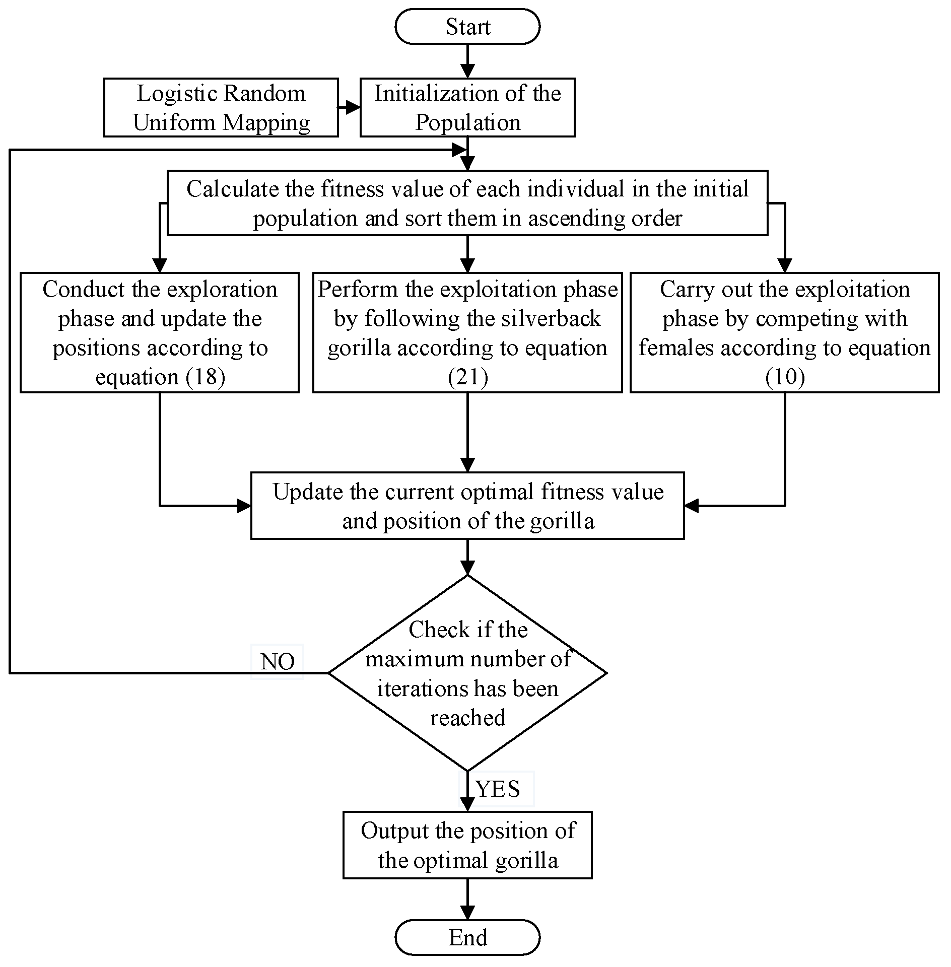
This paper improves the GTO algorithm based on the above strategies, balancing the algorithm's exploration and exploitation capabilities and enhancing the convergence speed. The improved algorithm is used to optimize the parameters of VMD and SVM. The specific process of the improved GTO algorithm is shown in Figure 1:

2.3. Improved Algorithm Testing

To validate the effectiveness and superiority of the improved GTO algorithm, it is tested on the single-peaked function F6 and the multi-peaked function F12 from the CEC2005 benchmark function set. The results are compared with the Whale Optimization Algorithm (WOA), Dung beetle optimization algorithm (DBO), Grey Wolf Optimizer (GWO), Northern Goshawk Optimization (NGO), Harris Hawks Optimization (HHO), the original GTO algorithm, and the improved GTO algorithm (OLGTO). Functions F6 and F12 are defined by equations (22) and (23), respectively.

F_{6} = Σ_{i = 1}^{n} {(| x_{i} + 0.5 |)}^{2}

(22)

\begin{array}{l} F_{12} (x) = \frac{π}{n} {10 \sin^{2} (π y_{1}) + \sum_{i = 1}^{n - 1} {(y_{i} - 1)}^{2} \\ [1 + 10 \sin^{2} (π y_{i + 1})] + {(y_{n} - 1)}^{2}} \\ + \sum_{i = 1}^{n} u (x_{i}, 10, 100, 4) \\ y_{i} = 1 + \frac{x_{i} + 1}{4} \\ u (x_{i}, a, k, m) = \{\begin{cases} k (x_{i} - a), x_{i} > a \\ 0, - a < x_{i} < a \\ k {(- x_{i} - a)}^{m}, x_{i} < a \end{cases} \end{array}

(23)

Where the dimensions and optimal minimum values for the F6 and F12 functions are 30 and 0, respectively. The search ranges for these functions are [-100, 100] and [-50, 50], respectively.

The population size and maximum number of iterations for the seven algorithms are uniformly set to 100 and 1000, respectively. In the OLGTO and GTO algorithms, the exploration probability p and control parameter Beta are set to 0.03 and 3, respectively. The weight factor W for GTO is set to 0.5. OLGTO employs a linear decreasing strategy and Levy flight strategy, with parameters

W_{\max} = 1.5

W_{\min} = 0.4

λ = 1.5

. The convergence results of the tested algorithms are shown in Figure 2.

In the entire search space, unimodal functions have only one global optimum and are primarily used to evaluate the algorithm's exploitation capability, i.e., its ability to converge to the optimal solution. Unimodal functions are relatively simple, allowing for clear measurement of convergence speed and accuracy. On the other hand, multimodal functions contain multiple local optima and are highly suitable for assessing the algorithm's exploration capability. Complex multimodal functions can test the algorithm's ability to avoid local optima and find the global optimum while evaluating the balance between exploration and exploitation. From the comparative results in Figure 2, it can be observed that for unimodal functions, the OLGTO algorithm consistently converges at a faster rate and ultimately achieves higher convergence accuracy than the other six algorithms. For multimodal functions, except for DBO and OLGTO, the WOA, GTO, GWO, NGO, and HHO algorithms all experience a significant decline in convergence speed after 200 iterations, falling into local optima and resulting in lower final convergence accuracy. Although the OLGTO algorithm shows a noticeable decrease in convergence speed around the 400th iteration, indicating a tendency to fall into local optima, it quickly resumes its convergence and reaches the optimal solution by the 579th iteration. This demonstrates the algorithm's strong balance between exploration and exploitation and its ability to escape local optima. In summary, the OLGTO algorithm exhibits strong adaptability compared to other algorithms, effectively avoiding local optima. This proves the effectiveness and superiority of the improved algorithm.

3. Fault Diagnosis Model Construction

3.1. VMD Fault Feature Extraction

Variational Mode Decomposition (VMD) is an improved method of the traditional Empirical Mode Decomposition (EMD), suitable for processing nonlinear and non-stationary signals. The principle of VMD is to decompose the original signal into a set of

K

intrinsic mode functions (IMFs), each with a central frequency. This decomposition is achieved through variational optimization. Additionally, VMD introduces Lagrange multipliers and a quadratic penalty factor

α

, and uses the Alternating Direction Method of Multipliers (ADMM) to solve the variational optimization problem to obtain the various modes and their corresponding central frequencies. By appropriately setting the total number of modes

K

and the value of the quadratic penalty factor

α

, VMD can overcome issues encountered by EMD when processing complex signals, such as mode mixing and endpoint effects, thereby enhancing VMD's adaptability to different signal decompositions. VMD is used for fault feature extraction in vibration signals, employing a composite index: permutation entropy/mutual information entropy as the fitness function. Permutation entropy reflects the complexity and irregularity of time series, with lower permutation entropy indicating more regular and periodic decomposed sequences [22]. Mutual information entropy measures the correlation between different information contained in different modes of VMD, with higher mutual information entropy indicating stronger correlation [23]. Therefore, the composite index of permutation entropy/mutual information entropy can balance the regularity and correlation of the decomposition modes. The calculation formulas for permutation entropy, mutual information entropy, permutation entropy/mutual information entropy, and the fitness value are shown in equations (24)-(27), respectively.

P E = - \sum (p (i) * \log (p (i)))

(24)

M I = \sum \sum [P (X, Y) * \log (P (X, Y) / (P (X) * P (Y)))]

(25)

C I = \frac{P E}{M I}

(26)

f i t n e s s = \min_{1 ~ K} {C I}

(27)

Where

p (i)

denotes the probability of the i-th permutation;

X

and

Y

are two random variables;

P (X, Y)

represents the joint probability distribution of

X

and

Y

;

P (X)

and

P (Y)

denote the marginal probability distributions of

X

and

Y

, respectively. When decomposing with VMD, the IMF component with the minimum fitness value is considered the current optimal IMF component. The mean, variance, peak value, kurtosis, root mean square, peak factor, impulse factor, waveform factor, and margin factor of the optimal IMF are then calculated, providing a 9-dimensional time-domain feature vector as the characteristic vector of the optimal IMF.

3.2. SVM Classification Model

Support Vector Machine (SVM) is a versatile supervised learning model widely applied in the field of fault diagnosis due to its efficient classification performance and its ability to handle high-dimensional data. The core idea is to find an optimal separating hyperplane that segregates samples of different classes. The regularization parameter

C

controls the trade-off between training error and margin, while the kernel parameter

σ

maps the data from a low-dimensional space to a high-dimensional space, making the sample data linearly separable in the high-dimensional space. Therefore, setting appropriate values for

C

and

σ

can enhance the model's generalization ability, avoid the complexity of high-dimensional computations, and thus improve the accuracy of fault diagnosis.

3.3. OLGTO-VMD-OLGTO-SVM Fault Diagnosis Model

To obtain suitable values for the number of modes

K

in the variational mode decomposition (VMD), the quadratic penalty factor

α

, the regularization parameter

C

, and the kernel parameter

σ

, and to effectively extract vibration signal features to improve the accuracy of fault diagnosis models, this paper proposes the use of the OLGTO algorithm. The OLGTO algorithm iteratively selects the optimal values for the critical parameters of the VMD and SVM models, establishing the OLGTO-VMD-OLGTO-SVM fault diagnosis model. The overall design process of the model is shown in Figure 3, with the specific steps as follows:

Step 1: Initialize the settings for the gorilla population size, the maximum number of iterations, and other relevant parameters.

Step 2: Distribute the gorilla population randomly and uniformly in the search space using the Logistic chaotic mapping. At this stage, the position vectors of the gorilla individuals represent the initial values of

α

K

C

, and

σ

Step 3: Use the composite metric of permutation entropy/mutual information entropy as the fitness function to calculate the initial fitness values of the gorilla individuals and sort them in ascending order to determine the optimal fitness value and position.

Step 4: Update the optimal fitness value and position according to formulas (18), (21), and (10) during the exploration and exploitation phases.

Step 5: Check if the current number of iterations exceeds the maximum number of iterations. If it does, the optimization process ends, and the optimal fitness value and position of the gorilla individuals, representing

α

K

C

, and

σ

, are outputted. Otherwise, return to Step 2 and continue the optimization process.

Step 6: Substitute the optimal parameters

α

and

K

into the VMD to extract features from the vibration signals. Divide the dataset into training and testing sets.

Step 7: Substitute the optimal parameters

C

and

σ

into the SVM to construct the fault diagnosis model and input the dataset to achieve fault diagnosis.

4. Fault Diagnosis Experiment Verification and Analysis

4.1. Data Preparation

In practical applications, it is necessary to consider the potential insufficiency of fault sample data. Therefore, fault diagnosis experiments utilize both the small-sample vibration data from the drive end of motor bearings from Case Western Reserve University and the large-sample vibration data from three-phase asynchronous motors to respectively verify the feasibility and superiority of the OLGTO-VMD-OLGTO-SVM fault diagnosis model.

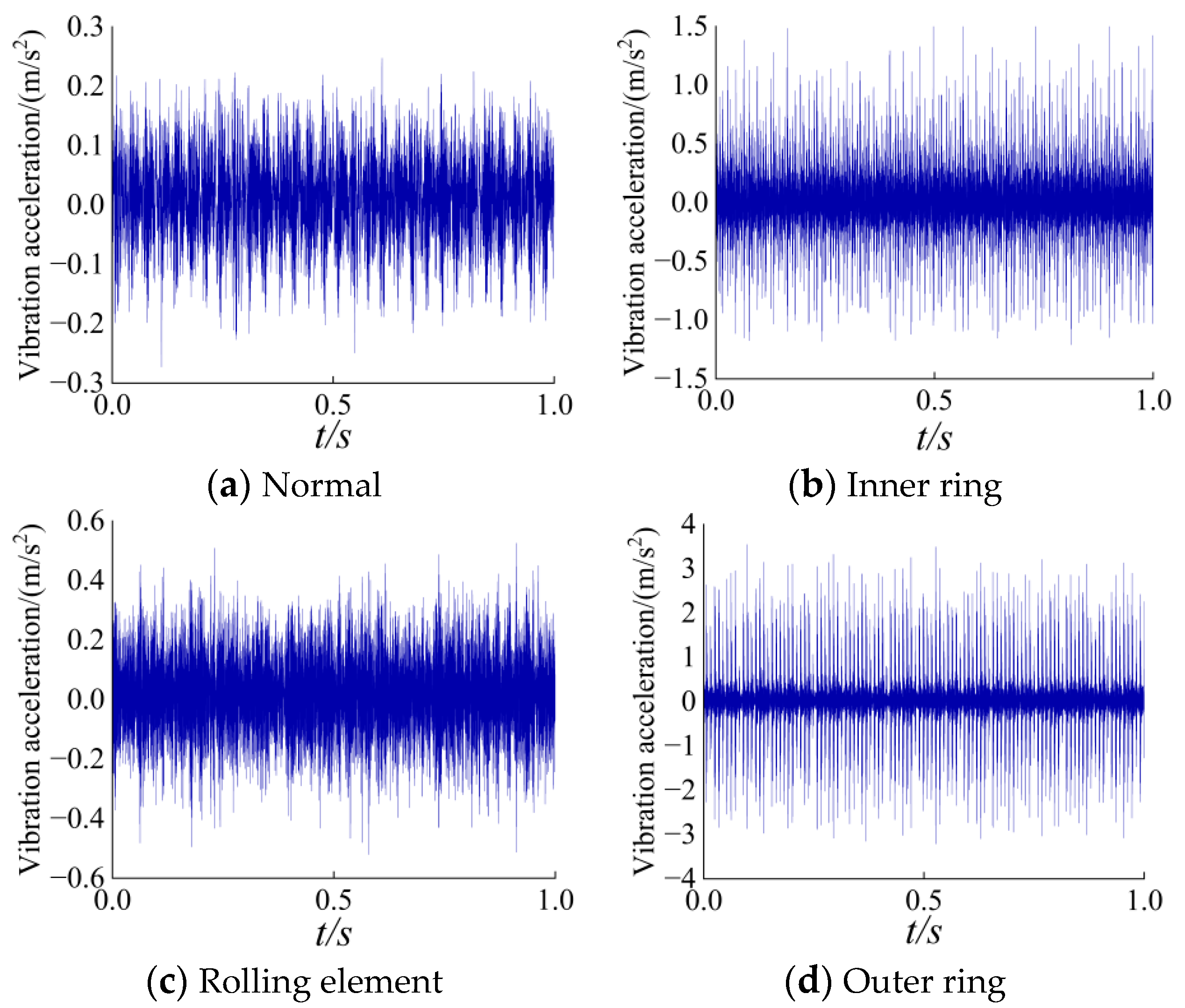
The motor bearing model from Case Western Reserve University is SKF6205, with single-point damage induced by electrical discharge machining. The sampling frequency is 12 kHz. The experiment considers the normal operating condition at 1797 rpm (labelled as 1) and nine fault conditions with different damage diameters: inner ring faults with diameters of 0.1778 mm, 0.3556 mm, and 0.5334 mm (labelled as 2, 5, and 8), outer ring faults with the same diameters (labelled as 3, 6, and 9), and rolling element faults with the same diameters (labelled as 4, 7, and 10). The vibration data in the time series is segmented using a sliding window, with a window size of 1000, and each sample contains 2048 data points. Each fault type includes 120 sample sets, resulting in a total of 1200 datasets used for the experiments. Due to space limitations, only the sampling signals within the first second of the normal condition and the inner ring fault, outer ring fault, and rolling element fault with a damage diameter of 0.1778 mm are shown in Figure 4.

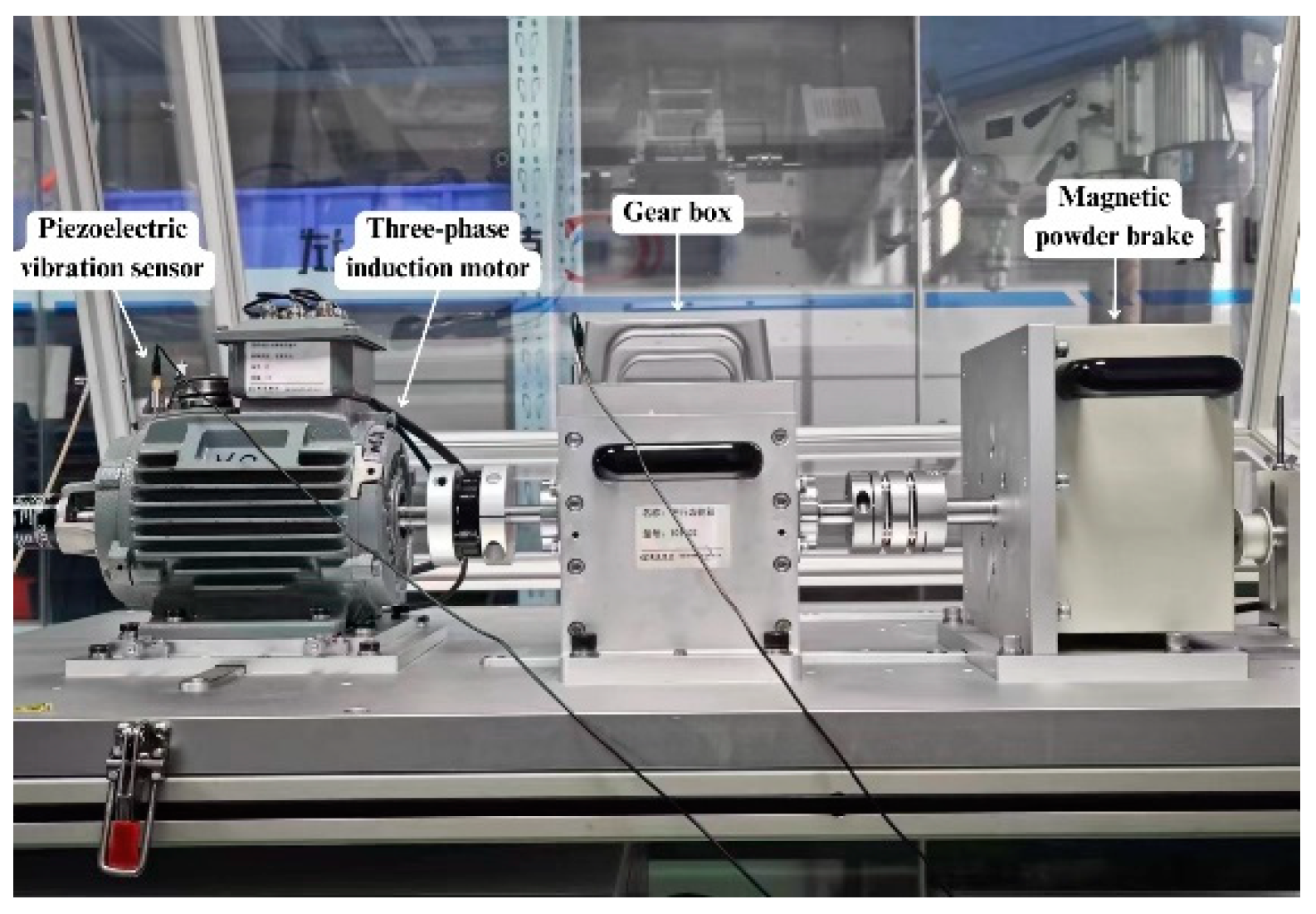
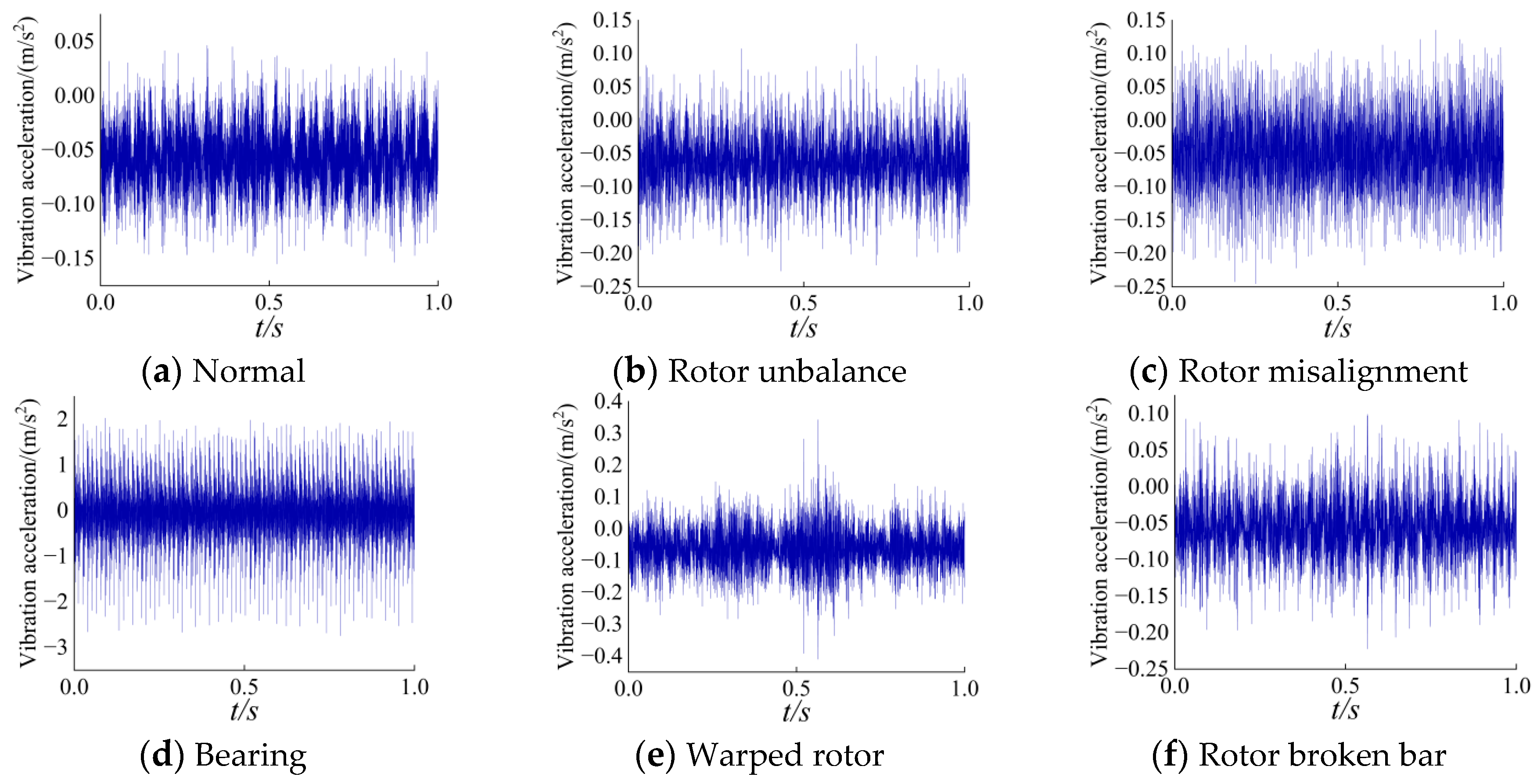
The data collection for the three-phase asynchronous motor is illustrated in Figure 5. The motor model is YXVF0M-2, with a sampling frequency of 5 kHz. The experiment considers the normal operating condition at 1500 rpm (labelled as 1) and five fault conditions: motor rotor imbalance (labelled as 2), motor rotor misalignment (labelled as 3), motor bearing fault (labelled as 4), motor rotor bend (labelled as 5), and motor rotor bar breakage (labelled as 6). The data is processed using the same sliding window method, with each sample containing 2048 data points. Each state includes 2000 sample sets, resulting in a total of 12000 datasets used for the experiments. The sampling signals within the first second of each state are shown in Figure 6.

4.2. Motor Bearing Fault Diagnosis Experiment

To validate the feasibility of the OLGTO-VMD-OLGTO-SVM method, four sets of experiments were conducted:(1) The motor bearing vibration signals were directly input into the SVM model for diagnosis.(2) The motor bearing vibration signals were directly input into the OLGTO-SVM model for diagnosis.(3) The motor bearing vibration signals were input into the SVM model for diagnosis after feature extraction using OLGTO-VMD.(4) The motor bearing vibration signals were input into the OLGTO-SVM model for diagnosis after feature extraction using OLGTO-VMD.

For experiments (1) and (2), the raw data were processed into a multi-dimensional sequence matrix of

1200 \times 2048

and input as

1 \times 2048

one-dimensional sequences into the SVM and OLGTO-SVM models, respectively. In experiment (1), the parameters

C

and

σ

were set to 3 and 1.5, respectively.

For experiments (3) and (4), the OLGTO algorithm was first used to optimize the parameters

α

and

K

in the VMD for feature extraction from the bearing vibration signals. The initial parameter settings are shown in Table 1. For each bearing state, 120 feature vectors were extracted (10 states in total, resulting in 1200 sets). The

1200 \times 2048

data samples were reduced to

1200 \times 9

feature vector samples after feature extraction. The OLGTO-VMD decomposition results are shown in Table 2.

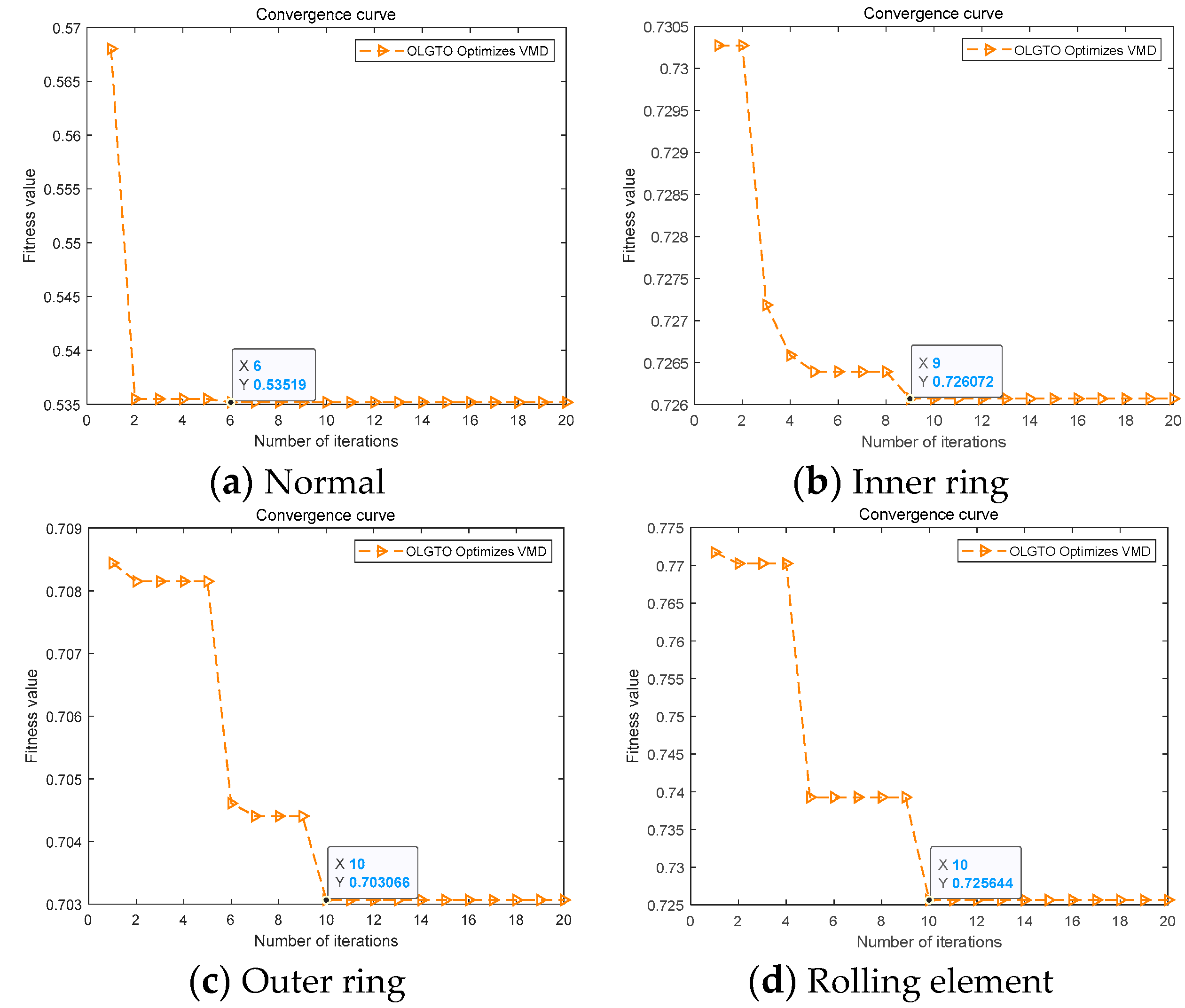
The iterative convergence curves are shown in Figure 7. Due to space limitations, only the convergence curves for the first four bearing states are displayed.

As shown in Table 2 and Figure 7, the total number of mode decompositions for each vibration signal is not less than 5, but the optimal IMF components are consistently IMF1 and IMF2. This indicates that the main characteristic components are fully extracted in the first few mode components after OLGTO-VMD decomposition. Additionally, for all 10 states, the optimal fitness values are achieved before the end of the iterations, demonstrating the algorithm's effective optimization performance.

Secondly, for each bearing state, the first 80 sets were used as the training set, and the last 40 sets were used as the testing set. The parameters

C

σ

, and data input method for experiment (3) were the same as those in experiment (1). For experiment (4), the training set samples were first input into the OLGTO-SVM model for training. The initial parameter settings for the OLGTO-SVM model are shown in Table 3. Through iteration, the optimal positions of the gorillas, representing the optimal parameters

C

and

σ

of the SVM, were obtained. The ultimate goal of fault diagnosis is to achieve accurate classification of different fault types. Therefore, the diagnostic accuracy as shown in equation (28) was used as the fitness function. The results of OLGTO optimizing the SVM parameters are shown in Table 4, and the fitness curves are shown in Figure 8.

A c c u r a c y = \frac{N_{c o r r e c t}}{N_{t o t a l}} \times 100 %

(28)

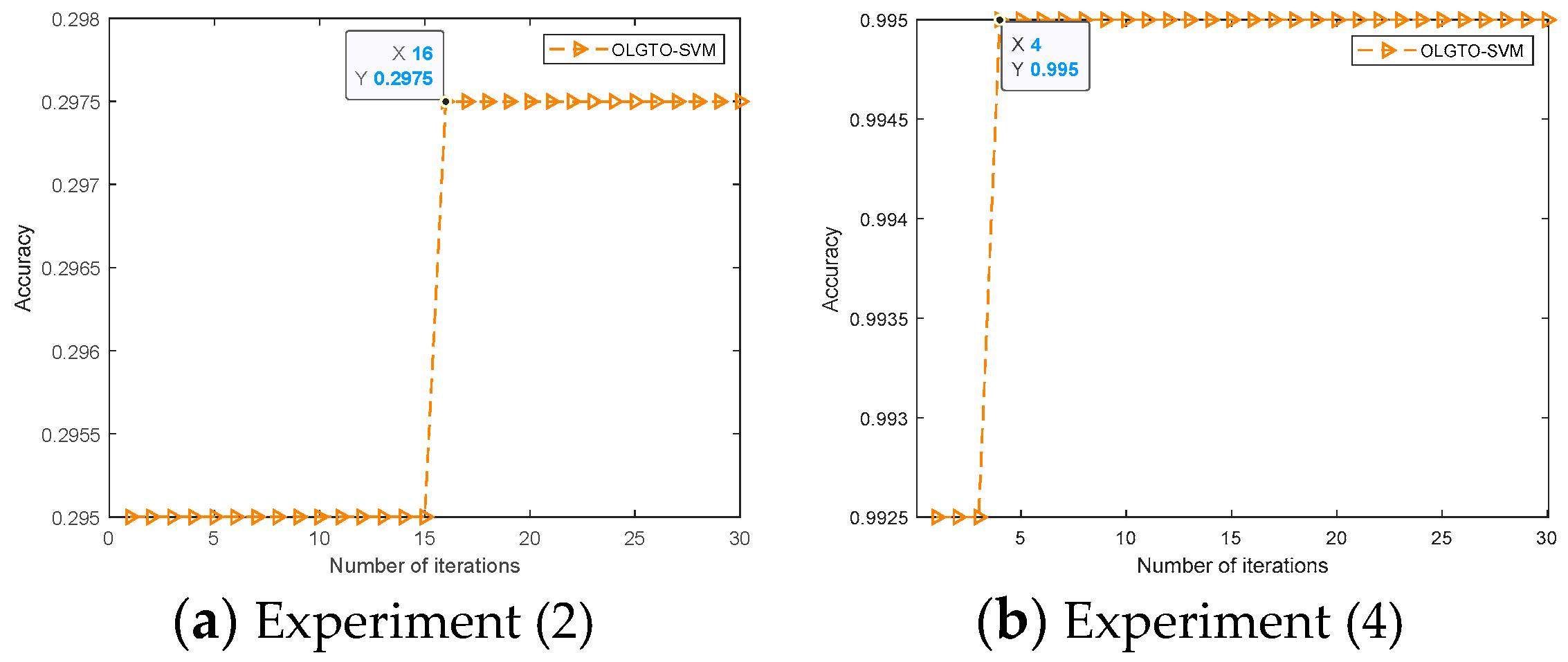
As shown in Figure 8, the fitness values for experiments (2) and (4) reach their optimum at the 16th and 3rd iterations, respectively, and remain stable thereafter. This indicates that the algorithm performs well in optimization. The optimal parameters and corresponding to the best fitness obtained through the iterative optimization of the OLGTO algorithm were used as the optimal parameters for the SVM model to test the sample data. The results of optimizing the SVM parameters are shown in Table 4.

In summary, the fault diagnosis results for experiments (1) through (4) are shown in Table 5.

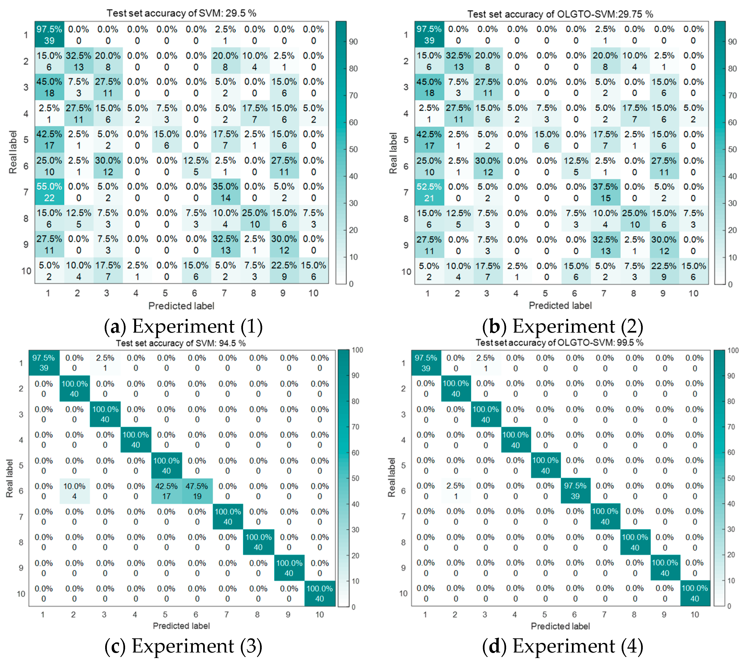
The confusion matrices for the fault diagnosis results are shown in Figure 9.

From the experimental results above, it can be seen that the SVM model performs poorly in identifying vibration signals without feature extraction. Even when optimized using OLGTO, there is no significant improvement in the final results. However, after feature extraction using the OLGTO-VMD method, the SVM achieves high diagnostic accuracy. Specifically, the OLGTO-VMD-OLGTO-SVM model achieves a diagnostic accuracy of 99.5%, which is a 5 percentage point improvement over the 94.5% accuracy of the OLGTO-VMD-SVM model. This validates the feasibility of applying the OLGTO-VMD-OLGTO-SVM method in fault diagnosis.

4.3. Fault Diagnosis Experiment of Three-Phase Asynchronous Motor

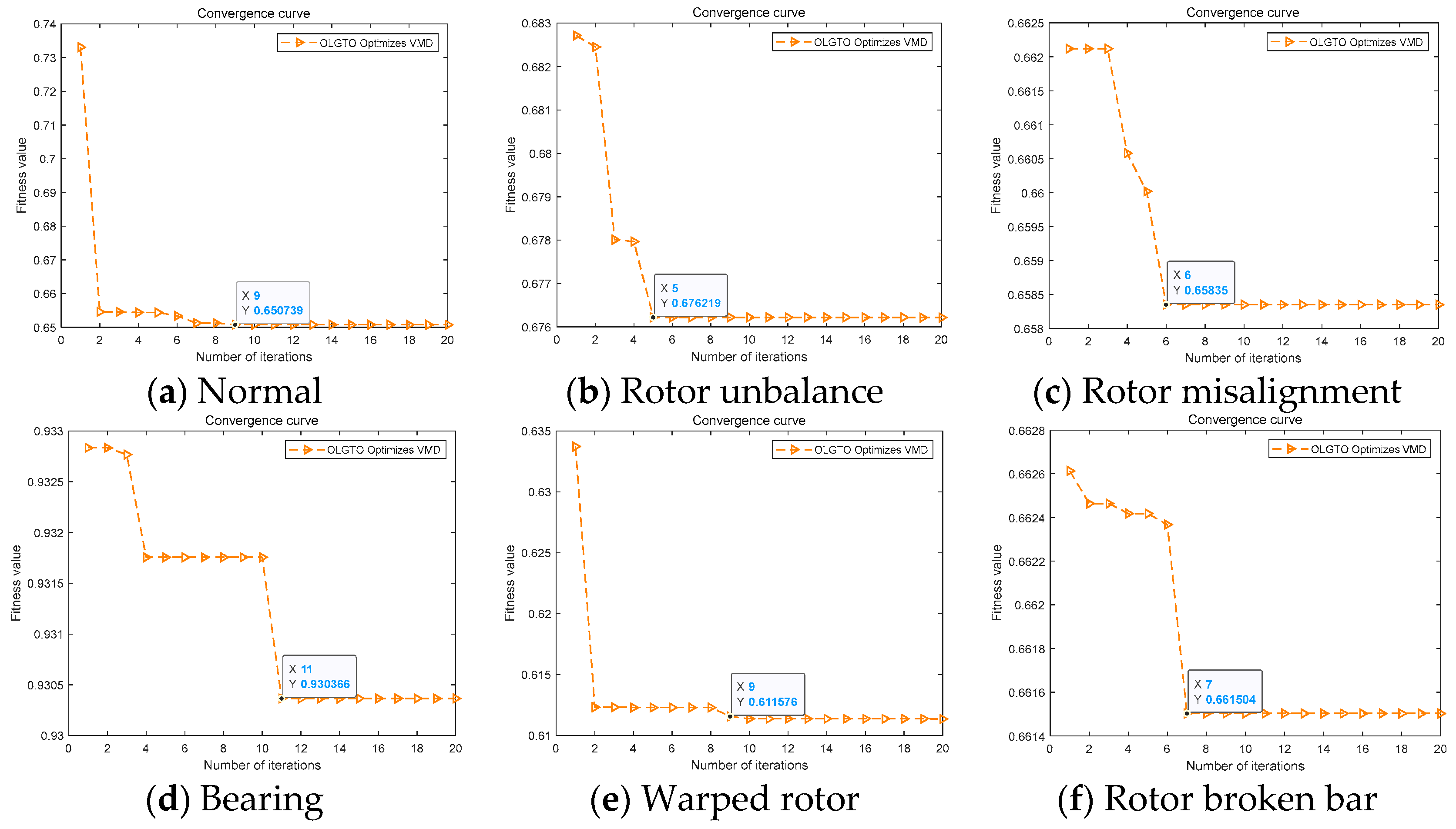
To validate the superiority of the OLGTO-VMD-OLGTO-SVM method, this method was compared with five other methods: OLGTO-VMD-CNN-BiLSTM (Convolutional Neural Network-Bidirectional Long Short-Term Memory), OLGTO-VMD-KNN (K-Nearest Neighbors), OLGTO-VMD-RF (Random Forest), OLGTO-VMD-BP (Back Propagation Neural Network), and OLGTO-VMD-ELM (Extreme Learning Machine). These six methods were applied to the fault diagnosis of an actual three-phase asynchronous motor, and their performance was compared. The experimental process was as follows: First, the vibration signals were processed using OLGTO-VMD to extract signal features. Then, the first 1200 sets of each motor state were used as the training set, and the last 800 sets were used as the testing set. These sets were input into OLGTO-SVM, CNN-BiLSTM, KNN, RF, BP, and ELM for training and diagnosis, respectively. The parameter settings for the OLGTO-VMD feature extraction were the same as those in Table 1. For each state of the three-phase asynchronous motor, 2000 feature vectors were extracted (6 states in total, resulting in 12000 sets). The

12000 \times 2048

sample data were reduced to

12000 \times 9

feature vector samples after feature extraction. The convergence curves of the parameter optimization iterations are shown in Figure 10, and the decomposition results of the motor vibration signals are shown in Table 6.

As shown by the decomposition results in Table 6, the total number of mode decompositions

K

for the three-phase asynchronous motor vibration signals is not less than 7, but the optimal IMF components are consistently IMF1 and IMF2. This indicates that the primary characteristic information of the vibration signals is concentrated in the first few IMF components after OLGTO-VMD decomposition. Furthermore, as observed from the convergence curves in Figure 10, the optimal fitness value for each state is achieved before the iterations are completed, demonstrating the algorithm's effective optimization performance.

After feature extraction, the multi-dimensional feature vector samples were obtained. These samples were input as one-dimensional sequences into OLGTO-SVM, CNN-BiLSTM, KNN, RF, BP, and ELM for training and diagnosis. The initial parameter settings for the OLGTO-SVM model were the same as those in Table 3. Using diagnostic accuracy as the fitness function, the parameter optimization results are shown in Figure 10.

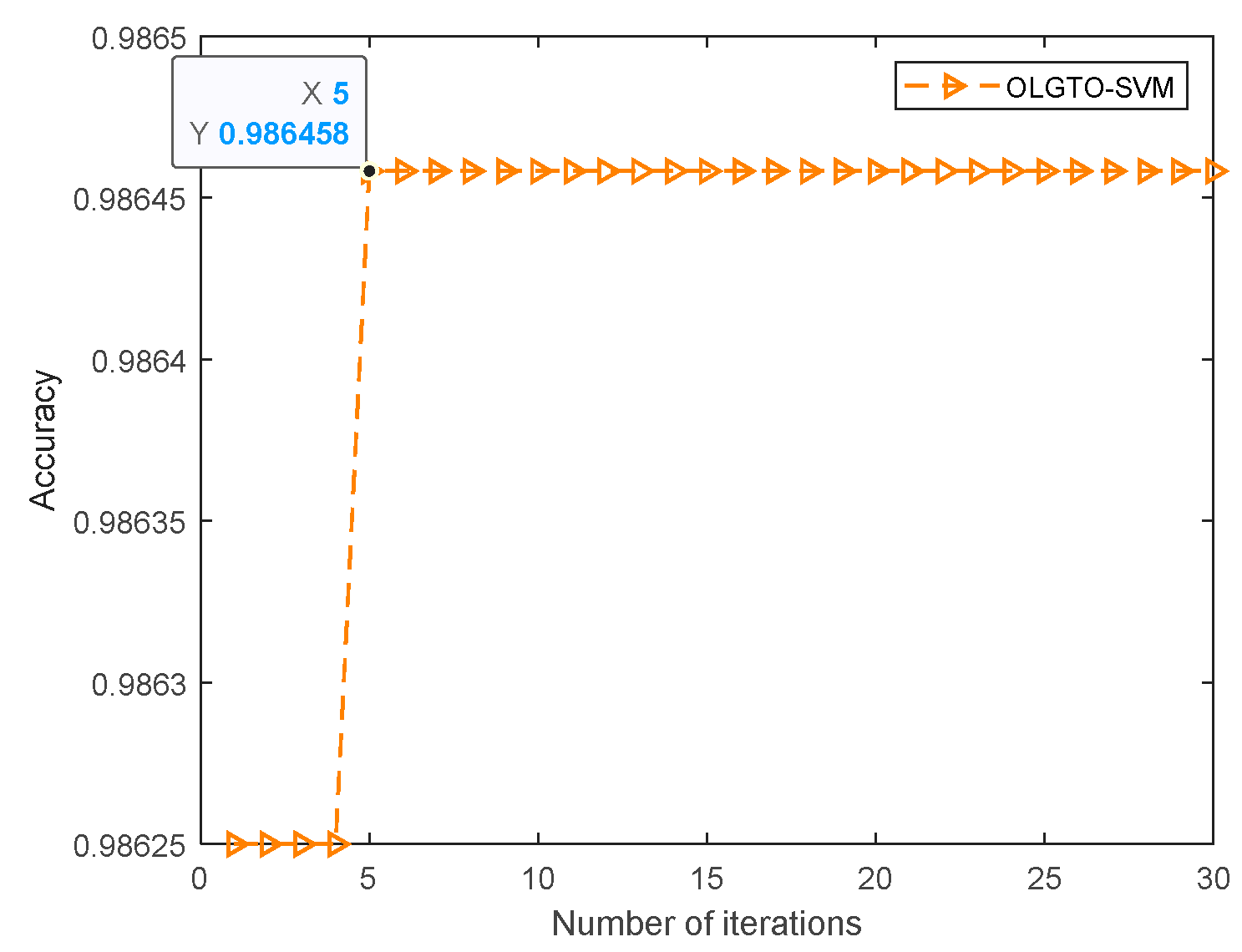
As shown in Figure 11, it can be observed that the fitness value reaches its optimum for the first time during the fifth iteration and remains stable thereafter with no fluctuations, indicating an overall stable trend. The optimal parameters

C

and

σ

obtained from the iterative optimization process of the OLGTO algorithm are then input into the SVM model to test the samples. The optimization results of the SVM model with the optimal parameters are shown in Table 7.

Additionally, the CNN-BiLSTM model was trained using the Adam optimizer with a maximum of 100 training epochs, an initial learning rate of 0.01, and a learning rate adjustment factor of 0.01 starting after 70 epochs. The regularization parameter was set to 0.001. The KNN model was constructed using the fitcknn function, with the number of nearest neighbors set to 1 and the distance metric type set to Euclidean. The RF model was constructed using the TreeBagger function with a minimum leaf size of 1, no out-of-bag predictions, no surrogate splits, and the number of decision trees set to 10. For the BP model, the optimal number of hidden layer nodes was set to 15. The hidden layer used the tansig activation function, the output layer used the purelin activation function, and the Levenberg-Marquardt algorithm was used as the training function. The maximum number of training iterations was set to 1000, with a learning rate of 0.1, a training goal error of 0.00001, a momentum factor of 0.01, a minimum gradient of 1e-6, and a maximum validation failure count of 6. The ELM model was used in regression mode with a sine activation function and 100 hidden layer nodes. The diagnostic results of the six methods are shown in Table 8.

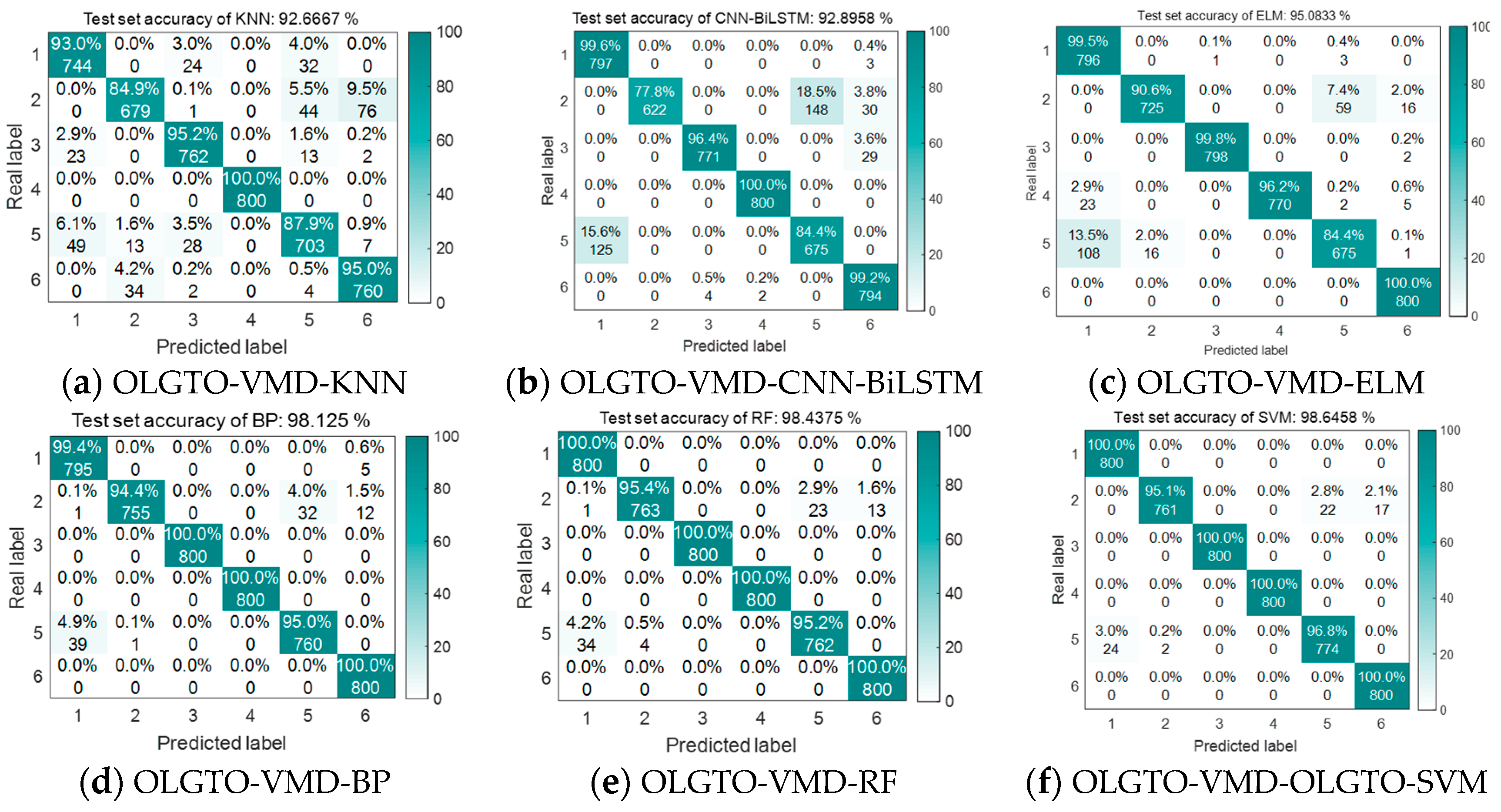
The confusion matrices for the diagnostic results of the six methods are shown in Figure 12.

From the comparison results above, it can be seen that despite the large data sample size, the OLGTO-VMD-OLGTO-SVM method still achieves a diagnostic accuracy of 98.6458%. This represents a significant improvement compared to the accuracies of 92.6667%, 92.8958%, and 95.0833% achieved by the OLGTO-VMD-KNN, OLGTO-VMD-CNN-BiLSTM, and OLGTO-VMD-ELM methods, respectively. While the improvements over OLGTO-VMD-BP and OLGTO-VMD-RF, which achieved 98.125% and 98.4375% accuracy, respectively, are smaller, it is important to note that a 0.3~0.5% increase in accuracy still represents a considerable number of data samples given the large sample size. Therefore, the method proposed in this paper is more reliable for practical applications, demonstrating the superiority of the OLGTO-VMD-OLGTO-SVM method.

5. Conclusion

(1) To address the deficiency of the Artificial Gorilla Troops Optimization (GTO) algorithm in the early iteration stages, where the numerous formula parameters hinder timely information exchange between gorillas, reducing the algorithm's global search capability and ability to escape local optima, and thus degrading convergence accuracy, improvements were made using Logistic chaotic mapping, a linear decreasing weight factor strategy, the global exploration strategy of the Osprey Optimization Algorithm, and the Levy flight strategy. Tests on unimodal and multimodal functions showed that the improved GTO algorithm possesses excellent global search capabilities and effectively avoids local optima.

(2) The selection of parameters

α

and

K

in VMD determines the effectiveness of vibration signal decomposition and feature extraction, while the parameters

C

and

σ

in SVM determine the final diagnostic accuracy. The improved GTO algorithm was used to optimize the parameters of both VMD and SVM, overcoming the difficulty of manually selecting optimal parameters and enhancing the generalization ability and adaptability of the fault diagnosis model.

(3) Fault diagnosis experiments on motor bearings and three-phase asynchronous motors validated the feasibility and superiority of the OLGTO-VMD-OLGTO-SVM method. This method can accurately identify fault types for both large and small sample data.

Author Contributions

H.Z.: Methodology, Validation, Formal analysis, Writing—original draft. T.F.: Writing—review and editing. L.M.: Investigation, Conceptualization, Project administration. All authors have read and agreed to the published version of the manuscript.

Funding

Please add: This research was funded by The National Natural Science Foundation Project (51007002); Anhui Industrial Internet Intelligent application and security engineering laboratory open fund (IASII21-05); Research on data synthesis and image detection methods for appearance defects of power equipment (QZ202108); Anhui University of Technology youth fund (QZ202109); Research on ship target recognition technology based on artificial intelligence (QZ202109).

Data Availability Statement

Dataset available on request from the authors.

Conflicts of Interest

The authors declare no conflicts of interest.

References

Khan, M.A.; Asad, B.; Vaimann, T.; Kallaste, A. An Advanced Diagnostic Approach for Broken Rotor Bar Detection and Classification in DTC Controlled Induction Motors by Leveraging Dynamic SHAP Interaction Feature Selection (DSHAP-IFS) GBDT Methodology. Machines 2024, 12, 495. [CrossRef]
Cureño-Osornio, Jonathan, et al. "Detection of Contamination and Failure in the Outer Race on Ceramic, Metallic, and Hybrid Bearings through AI Using Magnetic Flux and Current." Machines 12.8 (2024): 505.
Liu, C.; Zou, W.; Hu, Z.; Li, H.; Sui, X.; Ma, X.; Yang, F.; Guo, N. Bearing Health State Detection Based on Informer and CNN + Swin Transformer. Machines 2024, 12, 456. [CrossRef]
Zheng, J.; Su, M.; Ying, W.; Tong, J.; Pan, Z. Improved uniform phase empirical mode decomposition and its application in machinery fault diagnosis. Measurement 2021, 179. [CrossRef]
Yue, S.; Wang, Y.; Wei, L.; Zhang, Z.; Wang, H. The joint empirical mode decomposition-local mean decomposition method and its application to time series of compressor stall process. Aerosp. Sci. Technol. 2020, 105, 105969. [CrossRef]
Li, Y.-X.; Jiao, S.-B.; Gao, X. A novel signal feature extraction technology based on empirical wavelet transform and reverse dispersion entropy. Def. Technol. 2021, 17, 1625–1635. [CrossRef]
Liu, Q.; Yang, J.; Zhang, K. An improved empirical wavelet transform and sensitive components selecting method for bearing fault. Measurement 2022, 187. [CrossRef]
He, X.; Zhou, X.; Yu, W.; Hou, Y.; Mechefske, C.K. Adaptive variational mode decomposition and its application to multi-fault detection using mechanical vibration signals. ISA Trans. 2021, 111, 360–375. [CrossRef]
Gu, J.; Peng, Y.; Lu, H.; Chang, X.; Cao, S.; Chen, G.; Cao, B. An optimized variational mode decomposition method and its application in vibration signal analysis of bearings. Struct. Heal. Monit. 2022, 21, 2386–2407. [CrossRef]
Kumar, A.; Zhou, Y.; Xiang, J. Optimization of VMD using kernel-based mutual information for the extraction of weak features to detect bearing defects. Measurement 2021, 168, 108402. [CrossRef]
Yao, G.; Wang, Y.; Benbouzid, M.; Ait-Ahmed, M.; Yao, G.; Wang, Y.; Benbouzid, M.; Ait-Ahmed, M. A Hybrid Gearbox Fault Diagnosis Method Based on GWO-VMD and DE-KELM. Appl. Sci. 2021, 11, 4996. [CrossRef]
Liu, Zichang, et al. " Research on Fault Feature Extraction Method of Rolling Bearing Based on SSA–VMD–MCKD." Electronics 11.20 (2022): 3404.
Toma, R.N.; Prosvirin, A.E.; Kim, J.-M. Bearing Fault Diagnosis of Induction Motors Using a Genetic Algorithm and Machine Learning Classifiers. Sensors 2020, 20, 1884. [CrossRef]
Shao, Siyu, et al. "DCNN-based multi-signal induction motor fault diagnosis." IEEE Transactions on Instrumentation and Measurement 69.6 (2019): 2658-2669.
Guo, Z.; Liu, M.; Wang, Y.; Qin, H. A New Fault Diagnosis Classifier for Rolling Bearing United Multi-Scale Permutation Entropy Optimize VMD and Cuckoo Search SVM. IEEE Access 2020, 8, 153610–153629. [CrossRef]
Abdollahzadeh, B.; Gharehchopogh, F.S.; Mirjalili, S. Artificial gorilla troops optimizer: A new nature-inspired metaheuristic algorithm for global optimization problems. Int. J. Intell. Syst. 2021, 36, 5887–5958. [CrossRef]
Fadhil, M.S.; Farhan, A.K.; Fadhil, M.N. Designing Substitution Box Based on the 1D Logistic Map Chaotic System. IOP Conf. Series: Mater. Sci. Eng. 2021, 1076, 012041. [CrossRef]
Alawida, M. Enhancing logistic chaotic map for improved cryptographic security in random number generation. J. Inf. Secur. Appl. 2024, 80. [CrossRef]
Choudhary, S.; Sugumaran, S.; Belazi, A.; El-Latif, A.A.A. Linearly decreasing inertia weight PSO and improved weight factor-based clustering algorithm for wireless sensor networks. J. Ambient. Intell. Humaniz. Comput. 2023, 14, 6661–6679. [CrossRef]
Dehghani, M.; Trojovský, P. Osprey optimization algorithm: A new bio-inspired metaheuristic algorithm for solving engineering optimization problems. Front. Mech. Eng. 2023, 8. [CrossRef]
Kaidi, Wei, Mohammad Khishe, and Mokhtar Mohammadi. "Dynamic levy flight chimp optimization." Knowledge-Based Systems 235 (2022): 107625.
Ribeiro, M.; Henriques, T.; Castro, L.; Souto, A.; Antunes, L.; Costa-Santos, C.; Teixeira, A. The Entropy Universe. Entropy 2021, 23, 222. [CrossRef]
He J ,Qu L ,Wang P , et al.An oscillatory particle swarm optimization feature selection algorithm for hybrid data based on mutual information entropy[J].Applied Soft Computing,2024,152111261-.

Figure 1. Flowchart of improved artificial gorilla troop optimization algorithm.

Figure 2. Test algorithm convergence results.

Figure 3. Overall fault diagnosis process.

Figure 4. Bearing vibration signal waveform.

Figure 5. Three-phase asynchronous motor data acquisition.

Figure 6. Motor vibration signal waveform.

Figure 7. Convergence curve of OLGTO-VMD decomposition(bearing).

Figure 8. Fitness curve of OLGTO-SVM(bearing).

Figure 9. Troubleshooting results of experiments (1)-(4).

Figure 10. Convergence curve of OLGTO-VMD decomposition(Electric motors).

Figure 11. Fitness curve of OLGTO-SVM(Electric motors).

Figure 12. Results of 6 methods of diagnosis(Electric motors).

Table 1. OLGTO-VMD parameter settings.

Gorilla population size	Maximum iterations	Optimization parameters	Search range
15	20	$α$	$[100, 2500]$
15	20	$K$	$[3, 10]$

Table 2. OLGTO-VMD decomposition result(bearing).

Bearing status	$α$	$K$	Fitness value	Optimal IMF component
1	110	10	0.53519	IMF1
2	2104	10	0.72607	IMF2
3	110	9	0.70307	IMF1
4	2491	5	0.72564	IMF2
5	1989	7	0.75217	IMF1
6	1980	10	0.65067	IMF1
7	2271	10	0.66239	IMF1
8	2082	9	0.68290	IMF1
9	2372	10	0.68985	IMF1
10	2491	10	0.79858	IMF1

Table 3. OLGTO-SVM parameter Settings.

Gorilla population size	Maximum iterations	Optimization parameters	Search range
10	30	$C$	$[10^{- 3}, 10^{3}]$
10	30	$σ$	$[10^{- 8}, 10^{3}]$

Table 4. OLGTO-SVM parameter optimization results(bearing).

Algorithm model	Regularization parameter $C$	Kernel parameter $σ$	Experiment
OLGTO-SVM	471.6035	747.5808	(2)
OLGTO-SVM	20.2627	42.4093	(4)

Table 5. Comparison of experimental results of motor bearing fault diagnosis.

Methods	Accuracy
SVM	29.5%
OLGTO-SVM	29.75%
OLGTO-VMD-SVM	94.5%
OLGTO-VMD-OLGTO-SVM	99.5%

Table 6. OLGTO-VMD decomposition result(Electric motors).

Motor states	$α$	$K$	Fitness value	Optimal IMF component
1	2054	10	0.65074	IMF1
2	1176	7	0.67622	IMF1
3	2319	10	0.65835	IMF1
4	144	8	0.93037	IMF1
5	955	10	0.61136	IMF1
6	1545	7	0.661504	IMF1

Table 7. OLGTO-SVM parameter optimization results(Electric motors).

Algorithm model	Algorithm model $C$	Kernel parameter $σ$
OLGTO-SVM	81.4547	588.5758

Table 8. Comparison of experimental results of motor fault diagnosis.

Methods	Accuracy
OLGTO-VMD-KNN	92.6667%
OLGTO-VMD-CNN-BiLSTM	92.8958%
OLGTO-VMD-ELM	95.0833%
OLGTO-VMD-BP	98.125%
OLGTO-VMD-RF	98.4375%
OLGTO-VMD-OLGTO-SVM	98.6458%

Disclaimer/Publisher’s Note: The statements, opinions and data contained in all publications are solely those of the individual author(s) and contributor(s) and not of MDPI and/or the editor(s). MDPI and/or the editor(s) disclaim responsibility for any injury to people or property resulting from any ideas, methods, instructions or products referred to in the content.

© 2024 by the authors. Licensee MDPI, Basel, Switzerland. This article is an open access article distributed under the terms and conditions of the Creative Commons Attribution (CC BY) license (http://creativecommons.org/licenses/by/4.0/).

Copyright: This open access article is published under a Creative Commons CC BY 4.0 license, which permit the free download, distribution, and reuse, provided that the author and preprint are cited in any reuse.

MDPI Initiatives

Important Links

Choose an area of interest and we will send you notifications of new preprints at your preferred frequency.

Disclaimer

Research on Fault Diagnosis Method with Adaptive GTO Optimized VMD and SVM Parameters

Abstract

1. Introduction

2. Improved Artificial Gorilla Force Algorithm Fusing Osprey and Levy Flight (OLGTO)

2.1. The Original Artificial Gorilla Force Algorithm

2.2. Improved Artificial Gorilla Force Algorithm (OLGTO)

2.2.1. Logistic Chaotic Mapping Initializes Gorilla Population

2.2.2. Linearly Decreasing Weight Factors

2.2.3. Integrated Osprey Algorithm Global Exploration Strategy

2.2.4. Levy Flight Strategy

2.3. Improved Algorithm Testing

3. Fault Diagnosis Model Construction

3.1. VMD Fault Feature Extraction

3.2. SVM Classification Model

3.3. OLGTO-VMD-OLGTO-SVM Fault Diagnosis Model

4. Fault Diagnosis Experiment Verification and Analysis

4.1. Data Preparation

4.2. Motor Bearing Fault Diagnosis Experiment

4.3. Fault Diagnosis Experiment of Three-Phase Asynchronous Motor

5. Conclusion

Author Contributions

Funding

Data Availability Statement

Conflicts of Interest

References

MDPI Initiatives

Important Links

Subscribe