Compressible Diagnosis of the Membrane Fouling Based on the Transfer Entropy

1. Introduction

Membrane fouling is an important factor affecting wastewater treatment processes with membrane bioreactor (MBR), which can lead to the loss of membrane flux, deterioration of effluent quality, etc. [1,2,3]. To prevent this phenomenon, it is necessary to accurately diagnose the future case of membrane fouling before implementing efficient strategies [4,5]. However, in MBR, the biochemical process that triggers membrane fouling is complicated and involves amounts of causal variables, such as aeration, reflux, and dosing. The relationship between these variables is time-varying and nonlinear [6,7]. Therefore, it is challenging to establish an accurate diagnosis model for membrane fouling.

To establish the causal relationship between the variables and membrane fouling, some scholars have studied the mechanism of membrane fouling to diagnose its occurrence directly [8,9,10,11]. Lewis et al. analyzed the growth of filter cake in the process of low-pressure cross-flow microfiltration in MBR with fluid dynamics gauging [12]. Then, the diagnosis of membrane fouling was realized by quantifying the significance of membrane pore-level fouling phenomena at the early stage of filtration. In [13], a mechanism model was built for diagnosing membrane fouling by combining adenosine triphosphate and total cell count. The results displayed that this model was suitable for biological fouling diagnosis. In addition, MBR is affected by the flow distribution and hydraulic conditions in the reactor. A residence time distribution technique was developed to determine the impact of membrane geometry, orientation, and mixing efficiency on MBR performance [14]. Azizighannad et al. employed the Raman chemical image to identify the morphology of the membrane fouling [15]. This strategy could diagnose different types of membrane fouling with its observed appearance under specific static conditions. However, the above mechanism methods are difficult to adapt to different working conditions. Since the correction of a large number of parameters is complicated, they are time-consuming for maintaining model accuracy. To dissolve this problem, some data-driven diagnosis models, based on support vector regression (SVR), kernel function (KF) and artificial neural network (ANN) with strong adaptability, were established for membrane fouling [16,17,18,19]. For example, Liu et al. designed an SVR model with a LibSVM package to diagnose the case of membrane fouling in MBR by mapping the relationship between extracellular polymer substances, organic loading rate, transmembrane pressure difference and total membrane resistance [17]. The results showed that the relevant influencing factors of membrane fouling could be uncovered effectively. Han et al. proposed a multi-category diagnosis method based on KF for the detection and early warning of membrane fouling [18]. This method combined multiple binary classifiers to identify the causal variables of membrane fouling. Mittal et al. employed ANN to identify membrane fouling to minimize the risk of its occurrence [19]. The parameters of this model were updated based on the genetic algorithm, which was able to adapt to different operating conditions. The data-driven diagnosis models have the capability of sharpening the nonlinear relationship between input variables and output variables so that causal variables of membrane fouling can be distinguished. However, the existing models lack interpretability and struggle to straighten up interaction among different variables. Then, abundant variables with overlap and collinearity will increase the complexity and confusion of diagnosis.

To achieve a diagnosis process with interpretability, Chen et al. simplified the causality diagram through Granger causality and maximum spanning tree to diagnose the root causal variables of process abnormalities [20]. However, Granger causality analysis is only applicable to the causality analysis of linear processes, which cannot explain the nonlinearity in the membrane fouling. To conquer this challenge, Waghen et al. proposed a multi-level interpretable logic tree to clarify the nonlinear relationship between root causes, intermediate causes, and faults [21]. In addition, several intelligent tools are also introduced to explain the nonlinear process of membrane fouling. For example, Duan et al. developed an accident-relevance tree based on the analysis of the formation mechanism of quality accidents [22]. The method located the root causes of quality accidents utilizing the fuzzy mechanism and the vague nature of datasets. Velásquez et al. combined the decision tree learner and ANN to diagnose power transformer faults of membrane fouling, which reduced the calculation cost and improved the accuracy of fault classification simultaneously [23]. Other similar nonlinear methods can be observed in [24,25]. However, the methods mentioned in [21,22,23,24,25] only focus on the causality between local variables by constructing a tree causality diagram, rather than the interaction between all relevant variables. To provide the causal variables of faults comprehensively, Amin et al. synthesized principal component analysis (PCA) and Bayesian network to capture the nonlinear dependence of high-dimensional process data [26]. Then, the root causal variables of faults were diagnosed with the discretization of continuous data. In [27], a Bayesian network was developed to describe the relationship between alarm variables and root causal variables in thermal power plants. The parameters of the network were updated in a recursive way, which promoted to accurate detection of the root causal variables. Furthermore, Han et al. proposed recursive kernel PCA and Bayesian network to diagnose sludge bulking in the wastewater treatment process [28]. This method effectively captured the nonlinear and time-varying characteristics of sludge bulking to diagnose the root causal variables with high accuracy. However, once the diagnosis models in [26,27,28] are constructed with given datasets, they always hold the invariant information transfer path due to their complexity. When the operating conditions of MBR are changed frequently or drastically, it may be difficult to maintain acceptable accuracy for those models. Additionally, the relationship between those variables of membrane fouling exhibits both time-varying and nonlinear characteristics primarily because membrane fouling is a dynamic and complex process that is influenced by multiple, interacting factors. These characteristics can make it challenging to diagnose membrane fouling effectively.

Based on the above analysis, this paper proposes a compressible diagnosis model (CDM) based on transfer entropy. This model is used to depict the fault transfer topology (FTT) of membrane fouling and further explore the root cause following the operating conditions. The novelties of this work are as follows.

1) Based on the mechanism analysis associated with membrane fouling, the relationship between causal variables and membrane fouling is clarified with the feature extraction algorithm. Then, the related variables of membrane fouling are obtained under different operating conditions. Different from the data-driven diagnosis models in [15,16,17,18,19] with given causal variables, the feature extraction algorithm will enable the proposed CDM to transform raw data into informative representations that can be utilized for diagnosis.

2) Instead of using a mapping relationship with simple input-output representation such as the decision tree [21,22] and the Bayesian network [24,25], a topology based on transfer entropy is constructed. This approach not only provides a qualitative evaluation of the causal relationships between variables by observing the dynamic transfer path, but it also offers a quantitative description of those variables. It helps uncover the path of fault occurrence and further obtain the fault cause priority that may change over time as the operating conditions change.

3) The information compressible strategy (ICS) is designed to delete the redundant or repetitious affiliation relationship between the causal variables. With this strategy, the simplified FTT is obtained with low complexity during the update of fault transfer topology, which can maintain the diagnosis of membrane fouling speedily and accurately.

The rest of this paper is organized as follows. Section II introduces the background of membrane fouling. Section III introduces the diagnosis methods of membrane fouling in detail. Then, the experimental results of diagnosing membrane fouling are introduced in Section IV. Finally, Section V concludes this paper.

2. Background of Membrane Fouling

A. Membrane Fouling

Membrane fouling refers to the increase of water resistance and the decrease of permeation flux caused by the deposition of pollutants on the membrane surface or in its pores. The mechanisms of membrane fouling mainly include: (1) plugging of membrane pores by colloidal and SMP, fouling adhesion and gel layer formation; (2) formation and consolidation of the cake layer; (3) variation in pollutants due to long-term functioning of the reactor; (4) osmotic pressure effect. The membrane fouling has different characteristics, which can be divided into three types: (1) removable fouling, which usually generates in the filter cake layer and can be removed by physical means; (2) irremovable fouling, which usually requires chemical cleaning to remove the pore blockage; (3) irreversible fouling, which cannot be removed by any cleaning operation. In addition, there are various methods for studying membrane fouling, with the Hermia model being the most widely used. This semiempirical parametric model assigns physical significance to its parameters, which is effectively described by this model. The generalized Hermia model is a form of a nonlinear differential equation. It displays the dynamic of membrane fouling and its complex relationships between factors of membrane fouling. According to these characteristics, it is difficult to design a diagnosis method to diagnose the root cause of membrane fouling accurately.

B. Membrane Fouling Diagnosis System

The membrane fouling diagnosis system used for online locating root causal variables in the actual MBR wastewater treatment process is shown in Figure 1. The system consists of four modules: data acquisition module, feature extraction module, online prediction module, and online diagnosis module. The data acquisition module retrieves the value of process variables from sensors and transfers the acquired variables to the database via a programmable logic controller. The feature extraction module is designed to filter the collected process data. In this module, multiple related variables are selected as the preselected variables. Then, the partial least squares (PLS) method is used to reduce the dimension of the preselected variables to obtain the feature variables with a high correlation with the predicted variables. The online prediction module predicts the indicators for identifying membrane states. Finally, the online diagnosis module constructs an FTT to locate root causal variables. It is crucial to take corresponding measures to control membrane fouling.

3. Diagnostic Method of Membrane Fouling

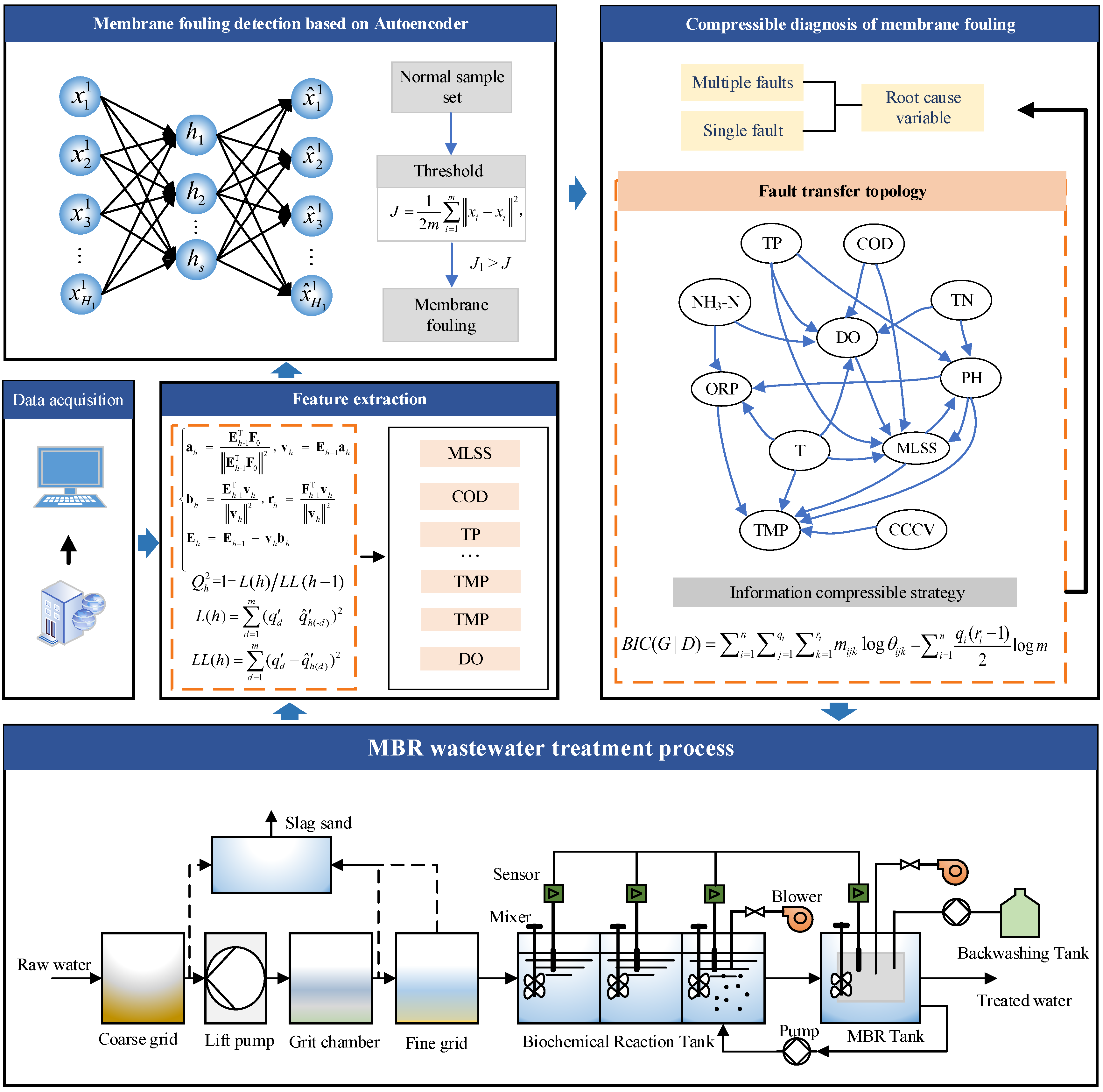
In this section, the CDM based on transfer entropy is proposed to diagnose membrane fouling. First, this method extracts relevant features, which preliminary simplifies the complexity of the system and focuses on key factors influencing membrane fouling. Second, the transfer entropy qualitative is calculated to quantify the causal transfer between different variables, and dynamically analyze the transfer path to form FFT. Finally, the root causal variable is found through the topology. With the design of the information compressible strategy, the causal relationship is further simplified between variables by deleting redundant or repetitive dependencies between causal variables.

A. Feature Variable Selection

In this part, the advantages of the linear regression algorithm and the typical PLS are integrated. Hence, the characteristic variables that have a great impact on membrane fouling detection can be selected. To be specific, the PLS algorithm is adopted in this study and the steps are as follows:

the data of the independent variable is given as P=[p₁,p₂,…,p_j], p_j= (p_1j, p_2j,…, p_ij)^T, i = 1,2,…,m, j = 1,2,…,n, and the dependent variable Q=[q₁, q₂,…, q_i]^T. The standard treatment is as follows:

$$\{\begin{array}{l}{p^{\prime }}_{ij}={\displaystyle \frac{p_{ij}-{\overline{p}}_j}{s_j}}\\ {q^{\prime }}_i={\displaystyle \frac{q_i-\overline{q}}{s}}\end{array},$$

(1)

where the standardized P and Q are recorded as E₀ and F₀. pʹ_ij and qʹ_i represent the elements in E₀ and F₀, respectively. p̅_j and s_j represent the average value and standard deviation of the elements in column j of P, respectively. q̅ and s represent the average value and standard deviation of all elements in Q, respectively. p̅_j and q̅ can be expressed by

$$\{\begin{array}{l}{\overline{p}}_j={\displaystyle \frac{1}{m}}{\displaystyle \sum _{i=1}^m{p}_{ij}},s_j=\sqrt{{\displaystyle \frac{1}{m-1}}{\displaystyle \sum _{i=1}^m{(p_{ij}-{\overline{p}}_j)}^2}}\\ \overline{q}={\displaystyle \frac{1}{m}}{\displaystyle \sum _{i=1}^m{q}_i,s=\sqrt{\frac{1}{m-1}{\displaystyle \sum _{i=1}^m{(q_i-\overline{q})}^2}}}\end{array}.$$

(2)

The principal component of the variable is found via the following formula:

$$\{\begin{array}{l}{a}_h=E_{h-1}^{\mathrm{T}}{F}_0/{\Vert E_{h-1}^{\mathrm{T}}{F}_0\Vert }^2\\ v_h=E_{h-1}{a}_h\\ b_h=E_{h-1}^{\mathrm{T}}{v}_h/{\Vert v_h\Vert }^2\\ r_h=F_{h-1}^{\mathrm{T}}{v}_h/{\Vert v_h\Vert }^2\\ E_h=E_{h-1}-v_h{b}_h\end{array},$$

(3)

where h is the number of extracted principal components. E_his the standardized independent variable matrix when h components are extracted. F_h is the standardized dependent variable matrix when h components are extracted. v_h is the component extracted from E_h-1. a_h, b_hand r_h represent the intermediate vectors.

The cross-validity $Q_h^2$ is used to determine the number of final extracted components with

$$Q_h^2=1-L(h)/LL(h-1),$$

(4)

where L(h) and LL(h) can be expressed by

$$L(h)={\displaystyle \sum _{d=1}^m{({q^{\prime }}_d-{\widehat{q^{\prime }}}_{h(-d)})}^2}，LL(h)={\displaystyle \sum _{d=1}^m{({q^{\prime }}_d-{\widehat{q^{\prime }}}_{h\left(d\right)})}^2},$$

(5)

where q’_d is the dth (0<d≤h+1) element in F₀, q̂’ represents the fitting quantity. Sample point d is deleted when modeling with the linear regression model, and h components are taken for regression modeling to obtain the coefficients α_i. Then, the fitting value of the dth sample point is calculated and recorded as q̂‘h_(-d). Besides, all sample points are used, and h components are taken for regression modeling to obtain coefficients ς_i. Finally, the fitting value of the dth sample point is calculated and recorded as q̂‘h_(d).

In the process of extracting components, when $Q_{k+1}^2$<0.0975 and the model accuracy reaches the expected requirements, the process of extracting components stops. The number of extracted principal components is m. And the feature variables are represented as X=[x₁,x₂,…,x_m].

B. Membrane Fouling Detection Model

Autoencoder (AE) is a multi-layer neural network of unsupervised learning in deep learning technique, which includes an encoder and a decoder (as shown in Figure 2). The encoder compresses the input data X=[x₁,x₂,…,x_m] to obtain the outputs of the hidden layer H=[h₁, h₂,…, h_s]. And the decoder takes the outputs of the hidden layer as the input and gets the output X̂= [x̂₁, x̂₂,…, x̂_m]. H can be expressed as

$$H=f(W_{x}X),$$

(6)

where f(x)=1/(1+e^-x) is the activation function. W_x represents the weight between the input layer and the hidden layer, and s<m. The output value X̂ can be expressed as

$$\stackrel{\wedge }{X}=f(W_{h}H),$$

(7)

where W_h is the weight between the hidden layer and the output layer.

The back-propagation algorithm is used to adjust the parameters of AE in the training process. For the input variable X=[x₁, x₂,…, x_m], the objective function is defined as

$$J={\displaystyle \frac{1}{2m}}{\displaystyle \sum _{i=1}^m{\Vert x_i-\widehat{x_i}\Vert }^2}.$$

(8)

To judge the existence of membrane fouling, the collected data samples for the autoencoder are tested after training. If the reconstruction error is greater than the threshold, it means the membrane fouling exists in the wastewater treatment process.

C. Construction of Fault Transfer Topology

Since transfer entropy can represent the direction of information transfer between variables, it can represent the relationship between fault variables. The transfer entropy is given as follows:

$$T(X_{i+1}|X,Y)={\displaystyle \sum _{x_{i+1},x_i,y_j}p(x_{i+1},x_i^{(k)},y_j^{(l)}){\log }_2\frac{p(x_{i+1}|x_i^{(k)},y_j^{(l)})}{p(x_{i+1}|x_i^{(k)})}},$$

(9)

where p(·|·) is the conditional probability. x_i and y_j represent the measured values of X and Y at time i and time j, respectively. X_i+1 represents the measured value of X at the next time. k and l are the implantation dimensions of X and Y, respectively. The transfer entropy represents the influence of the existence of y_j on the state of x_i+1.

By calculating the transfer entropy between preselected variables, the information transfer relationship between all variables can be obtained. The transfer entropy of Y to X is different from X to Y, which shows that there are differences in the amount of information transferred in two directions. It reflects the difference in the degree of interaction between variables. The direction of causality between variables can be determined by the difference of two transfer entropy:

$$T_{Y\to X}=T(X_{i+1}|X,Y)-T(Y_{i+1}|Y,X).$$

(10)

If T_Y→X is positive, it means that Y has a greater impact on the information entropy of X than the impact X has on the information entropy of Y. At this time, Y is the causal variable of X. On the contrary, if T_Y→X is negative, it means that X is the causal variable of Y.

The transfer entropy between all selected variables is calculated to determine the causality, which can build an adjacency matrix A∊R^k×k. Then, the position in the adjacency matrix A is determined according to the direction of causality between variables. If T_Y→X is positive, it means Y is the causal variable of X. The value of T_Y→X is placed in row Y and column X of A:

$$A=\left(\begin{array}{ccccc}0& \dots & 0& \dots & T_{1\to a}\\ ⋮& \ddots & ⋮& \ddots & ⋮\\ T_{a\to 1}& \cdots & 0& \cdots & 0\\ ⋮& \ddots & ⋮& \ddots & ⋮\\ 0& \dots & T_{a\to b}& \dots & 0\end{array}\right),$$

(11)

where the diagonal value of A is 0. T_a→1 means that the ath variable is the causal variable of the first variable. In turn, the value of T_1→a is 0.

Thus, the adjacency matrix between variables can be obtained, and the related variables can be connected by lines according to the values in the matrix to obtain the fault transfer topology. After determining the causal relationship between all variables, FTT can be obtained as shown in Figure 3.

D. Simplification of Fault Propagation Topology

FTT expresses the complex relationship between the variables, which will affect the search for the root causal variables of membrane fouling. Therefore, it is necessary to simplify this topology to identify the main impact relationships.

When X and Y are disrupted, a new sequence is constructed as follows:

$$\{\begin{array}{l}{X}^s=[X_i,X_{i+1},\mathrm{...},X_{i+M-1}]\\ Y^s=[Y_j,Y_{j+1},\mathrm{...},Y_{j+M-1}]\end{array},$$

(12)

where M is the number of samples of the new sequence, and N is the total number of samples of the original sequence. The value range of i and j is [1, N-M+1].

The new sequence is a subset of the original sequence. The statistical characteristics in the stationary sequence are the same as those in the original sequence. To ensure no correlation between the two sequences, i and j need to meet ||i-j||≥e, where e is a sufficiently large integer. Then the new sequence formula has two variables with a large time interval. It can be considered that the correlation between the two variables is eliminated by a large time interval. Thus, two variable sequences without causality are obtained. The transfer entropy te_s of the multiple sets of such new sequences are calculated and stored in NET with NET = [te₁, te₂ ,…, te_s]. Then, the significance threshold is calculated by

$$S_{Y\to X}={\mu }_{NET}+3{\sigma }_{NET},$$

(13)

where µ_NET is the mean value of NET and σ_NET is the standard deviation of NET. The greater difference in transfer entropy than the threshold value represents that there is a causal relationship between variables.

To further simplify the fault transfer topology, an ICS based on a BIC score function is proposed. The designed ICS mainly includes two parts. First, the fitting degree is considered. Then, the complexity of the structure is reduced to avoid the decline in diagnosis accuracy caused by complex models and many other parameters.

For the dataset D = {D₁, D₂, D₃,…, D_m}, m represents the size of the sample dataset. The logarithmic likelihood function of the parameter θ can be expressed as:

$$I(\theta |D)={\displaystyle {\sum }_{l=1}^m\log P(D_l|\theta )}={\displaystyle {\sum }_{i=1}^n{\displaystyle {\sum }_{j=1}^{q_i}{\displaystyle {\sum }_{k=1}^{r_i}{m}_{ijk}\log {\theta }_{ijk}}}},$$

(14)

where θ ={θ_ijk|i=1,2,…,n, j=1,2,…,q_i, k=1,2,…,r_i}. θ_ijk represents the probability that the value of node X_i is k when the parent node value of node X_i is j. q_i represents the total number of parent node set values of node X_i, and q_i = 1 when node X_i has no parent node. r_i represents the number of possible value types of node X_i, and m_ijk represents the number of samples that meet X_i = k and the parent node is j in D.

The ICS based on the BIC score function can be expressed as

$$BIC(G|D)=I(\theta |D)-{\displaystyle {\sum }_{i=1}^n\frac{q_i(r_i-1)}{2}\log m},$$

(15)

where BIC(G|D) represents the score for structure G. Through ICS, the indirect connection of variables is scored to determine whether to delete. The presentation of the indirect connection is shown in Figure 4. Then, the simplified FTT is obtained after using ICS.

The information relevance strategy is proposed to find the root causal variables. The main idea of information relevance is to select a node as the starting node arbitrarily, and calculate the sum of transfer entropy of the remaining paths. When the sum of transfer entropy has the maximum value, the variable represented by this node is the root causal variable. The sum of transfer entropy can be expressed as

$$K_i={\displaystyle {\sum }_{v=1}^N{T}_v(X_{i+1}|X,Y)},$$

(16)

where K_i represents the sum of the transfer entropy of all paths when the ith node is the starting node. N is the number of paths of the current structure, and T_v represents the transfer entropy corresponding to the vth path. Therefore, the corresponding node variable is selected as the root causal variable when K_i takes the maximum value. The specific steps of membrane fouling diagnosis are shown in Table 1. Additionally, the change in operating conditions will lead to changes in the input distribution of CDM. This means that the potential relationship between process variables will change, the insignificant variables that previously led to membrane fouling may become the root cause and effect variables of the fault. The proposed CDM has two mechanisms to perceive this kind of scenario: 1) The least square method in the process of feature extraction will produce new principal components, which may lead to changes in the composition and number of filtered variables. 2) After recalculating the transfer entropy of the fault variable, FFT will obtain a completely different causal relationship. When these scenarios happen, the steps of membrane fouling diagnosis will be refreshed.

4. Experimental Studies

The effectiveness of CDM is verified in an actual WWTP. The performance of this method is evaluated by diagnosis accuracy (DA). All the simulation experiments were programmed with MATLAB version 2018 and run on a PC with one clock speed of 3.0 GHz and 8 GB of RAM under a Microsoft Windows 10 environment. All data were acquired in real WWTPs from January 1, 2016, to February 27, 2016. 2000 groups of data were selected as samples.

A. Feature Variable Selection

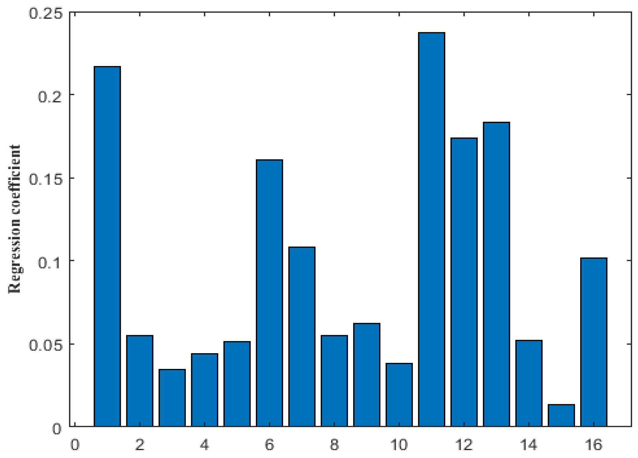
In this experiment, 5000 normal data samples, collected in the actual WWTP, are used to select the feature variables. Chemical oxygen demand (COD), influent NH₃-N, influent flow volume, NO₃-N in the anoxic zone, influent total phosphorus (TP), oxidation-reduction potential (ORP) in the anaerobic zone, mixed dissolved oxygen (DO) in the aerobic zone, sludge concentration in the aerobic zone, effluent flow volume, liquor suspended solid of the aerobic zone, aeration, effluent turbidity, water temperature, pH, F/M of aerobic zone, transmembrane pressure (TMP) are replaced by numbers 1 to 16, which are selected as pre-selected fault variables in this experiment. The regression coefficient in the obtained regression equation was expressed as the correlation between independent and dependent variables. The coefficients corresponding to all independent variables are shown in Figure 5.

By sorting the coefficients, 12 variables with large regression coefficients are selected as the inputs of the membrane fouling detection model and membrane fouling diagnosis model, which are COD, influent NH₃-N, influent TP, ORP in the anaerobic zone, DO in the aerobic zone, sludge concentration in the aerobic zone, effluent flow, aeration, effluent turbidity, water temperature, pH and TMP.

B. Membrane Fouling Detection Model

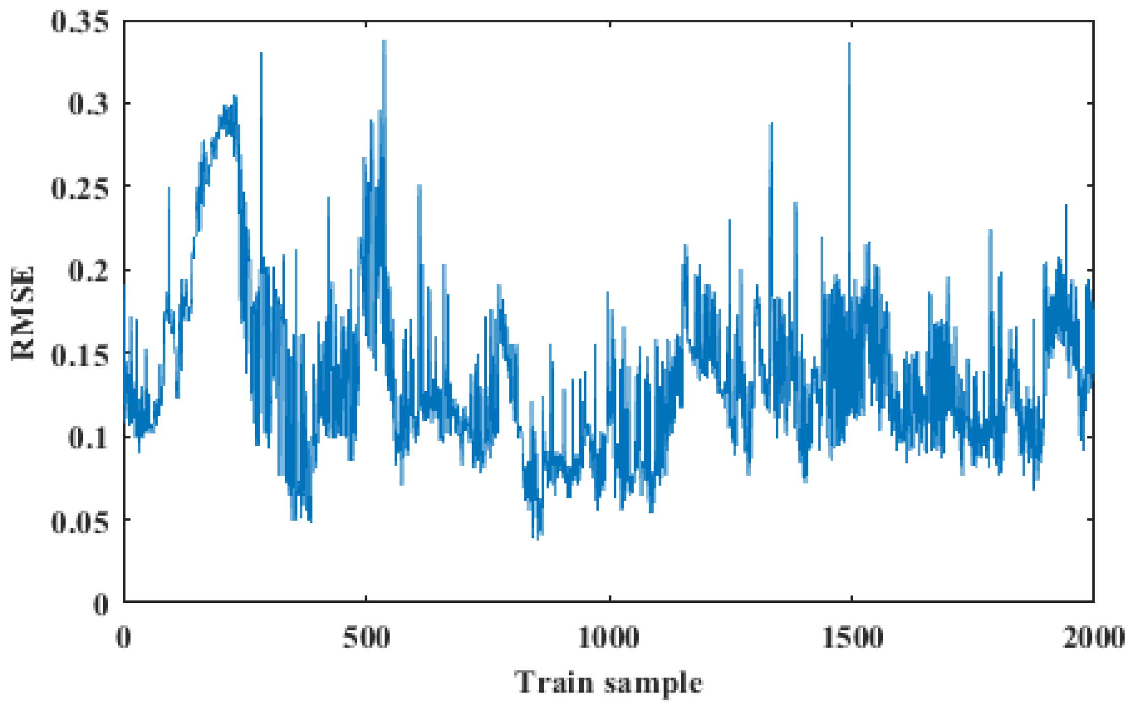
In this part, 2000 samples of selected variables are used in the training dataset. 800 samples of selected variables are used in the test dataset. The number of nodes in the input layer and output layer of the Autoencoder is 12, and the number of nodes in the hidden layer is 5. The threshold can be determined by the maximum root mean square error in the training process of normal data samples.

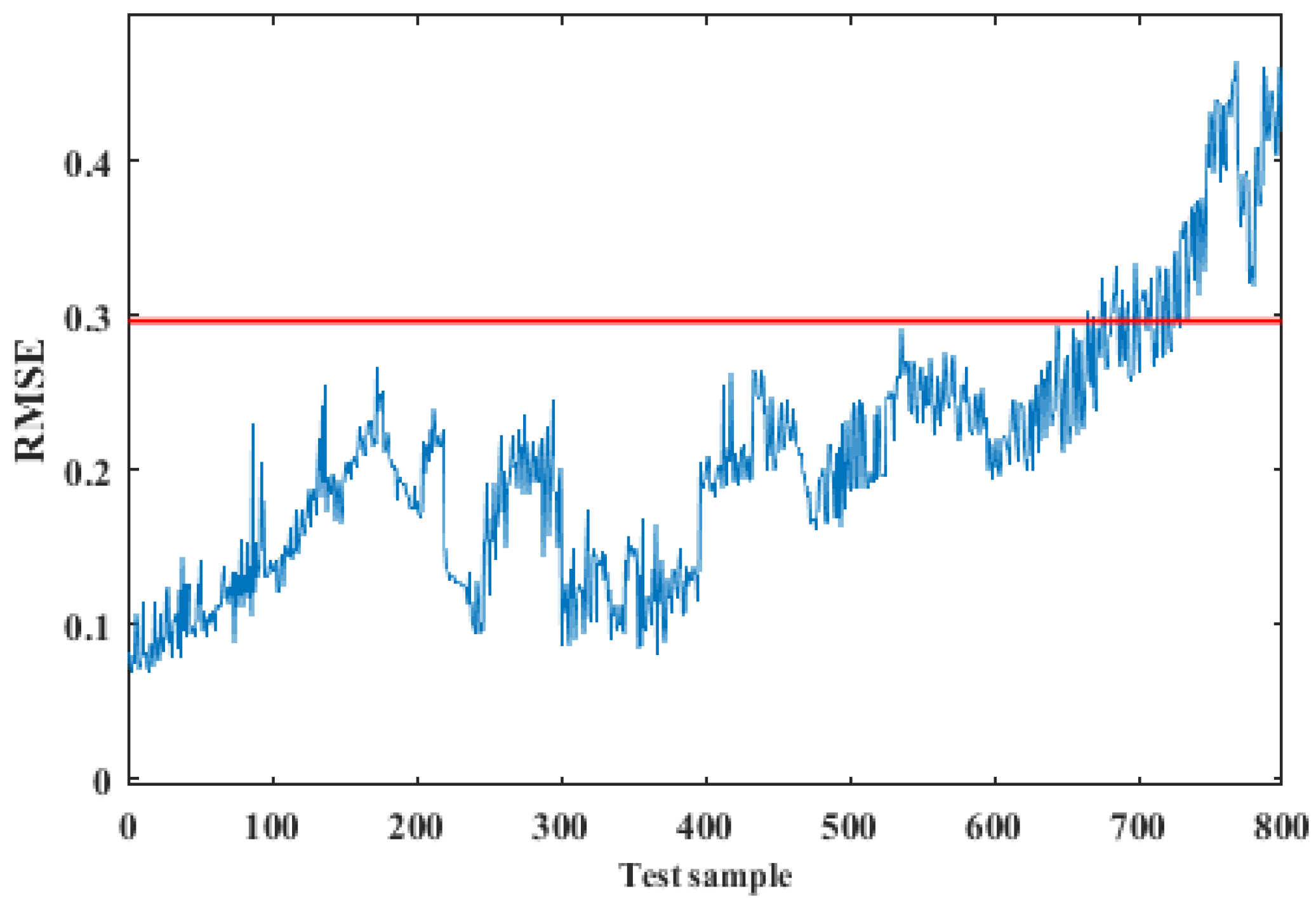
The experimental results are shown in Figure 6 and Figure 7. The maximum RMSE of the normal training samples in Figure 6 is used as the threshold, which is shown as the red line in Figure 7. It can be found from Figure 7 that the data samples from 0 to 650 are under normal conditions, while membrane fouling happens in the data samples from 650 to 800. Therefore, it can prove the effectiveness of this method.

$$A_1=\left(\begin{array}{c}\begin{array}{rrrrrrrrrrrr}\hfill 0& \hfill 0& \hfill 0& \hfill 0.810403& \hfill 0.464642& \hfill 0.057451& \hfill 0.942594& \hfill 1.247714& \hfill 0.192291& \hfill 0.11872& \hfill 0.094991& \hfill 1.058295\\ \hfill 0.010245& \hfill 0& \hfill 0& \hfill 0.730733& \hfill 0.43716& \hfill 0.05863& \hfill 1.000398& \hfill 1.228595& \hfill 0.20512& \hfill 0.134615& \hfill 0.122252& \hfill 1.100775\\ \hfill 0.016909& \hfill 0.001415& \hfill 0& \hfill 0.403387& \hfill 0.28396& \hfill 0.031732& \hfill 0.611236& \hfill 0.579717& \hfill 0.133133& \hfill 0.047092& \hfill 0.073589& \hfill 0.639023\\ \hfill 0& \hfill 0& \hfill 0& \hfill 0& \hfill 0& \hfill 0& \hfill 0.255535& \hfill 0.470007& \hfill 0& \hfill 0& \hfill 0& \hfill 0.394362\\ \hfill 0& \hfill 0& \hfill 0& \hfill 0.476931& \hfill 0& \hfill 0& \hfill 0.822288& \hfill 1.030058& \hfill 0.010018& \hfill 0& \hfill 0& \hfill 0.958113\\ \hfill 0& \hfill 0& \hfill 0& \hfill 0.756785& \hfill 0.276084& \hfill 0& \hfill 0.90815& \hfill 1.065932& \hfill 0.121703& \hfill 0.003572& \hfill 0& \hfill 1.030733\\ \hfill 0& \hfill 0& \hfill 0& \hfill 0& \hfill 0& \hfill 0& \hfill 0& \hfill 0.244137& \hfill 0& \hfill 0& \hfill 0& \hfill 0.155584\\ \hfill 0& \hfill 0& \hfill 0& \hfill 0& \hfill 0& \hfill 0& \hfill 0& \hfill 0& \hfill 0& \hfill 0& \hfill 0& \hfill 0\\ \hfill 0& \hfill 0& \hfill 0& \hfill 0.22354& \hfill 0& \hfill 0& \hfill 0.306308& \hfill 0.342152& \hfill 0& \hfill 0& \hfill 0& \hfill 0.311331\\ \hfill 0& \hfill 0& \hfill 0& \hfill 0.852613& \hfill 0.355963& \hfill 0& \hfill 1.032178& \hfill 1.267596& \hfill 0.1403& \hfill 0& \hfill 0& \hfill 1.146267\\ \hfill 0& \hfill 0& \hfill 0& \hfill 0.846681& \hfill 0.325523& \hfill 0.009613& \hfill 1.018529& \hfill 1.201856& \hfill 0.212144& \hfill 0.01461& \hfill 0& \hfill 1.119884\\ \hfill 0& \hfill 0& \hfill 0& \hfill 0& \hfill 0& \hfill 0& \hfill 0& \hfill 0.140916& \hfill 0& \hfill 0& \hfill 0& \hfill 0\end{array}\end{array}\right)$$

(17)

$$A_2=\left(\begin{array}{c}\begin{array}{rrrrrrrrrrrr}\hfill 0& \hfill 0& \hfill 0& \hfill 0.810403& \hfill 0& \hfill 0& \hfill 0.942594& \hfill 1.247714& \hfill 0& \hfill 0& \hfill 0& \hfill 1.058295\\ \hfill 0& \hfill 0& \hfill 0& \hfill 0.730733& \hfill 0& \hfill 0& \hfill 1.000398& \hfill 1.228595& \hfill 0& \hfill 0& \hfill 0& \hfill 1.100775\\ \hfill 0& \hfill 0& \hfill 0& \hfill 0& \hfill 0& \hfill 0& \hfill 0& \hfill 0& \hfill 0& \hfill 0& \hfill 0& \hfill 0\\ \hfill 0& \hfill 0& \hfill 0& \hfill 0& \hfill 0& \hfill 0& \hfill 0& \hfill 0& \hfill 0& \hfill 0& \hfill 0& \hfill 0\\ \hfill 0& \hfill 0& \hfill 0& \hfill 0& \hfill 0& \hfill 0& \hfill 0.822288& \hfill 1.030058& \hfill 0& \hfill 0& \hfill 0& \hfill 0.958113\\ \hfill 0& \hfill 0& \hfill 0& \hfill 0.756785& \hfill 0& \hfill 0& \hfill 0.90815& \hfill 1.065932& \hfill 0& \hfill 0& \hfill 0& \hfill 1.030733\\ \hfill 0& \hfill 0& \hfill 0& \hfill 0& \hfill 0& \hfill 0& \hfill 0& \hfill 0& \hfill 0& \hfill 0& \hfill 0& \hfill 0\\ \hfill 0& \hfill 0& \hfill 0& \hfill 0& \hfill 0& \hfill 0& \hfill 0& \hfill 0& \hfill 0& \hfill 0& \hfill 0& \hfill 0\\ \hfill 0& \hfill 0& \hfill 0& \hfill 0& \hfill 0& \hfill 0& \hfill 0& \hfill 0& \hfill 0& \hfill 0& \hfill 0& \hfill 0\\ \hfill 0& \hfill 0& \hfill 0& \hfill 0.852613& \hfill 0& \hfill 0& \hfill 1.032178& \hfill 1.267596& \hfill 0& \hfill 0& \hfill 0& \hfill 1.146267\\ \hfill 0& \hfill 0& \hfill 0& \hfill 0.846681& \hfill 0& \hfill 0& \hfill 1.018529& \hfill 1.201856& \hfill 0& \hfill 0& \hfill 0& \hfill 1.119884\\ \hfill 0& \hfill 0& \hfill 0& \hfill 0& \hfill 0& \hfill 0& \hfill 0& \hfill 0& \hfill 0& \hfill 0& \hfill 0& \hfill 0\end{array}\end{array}\right)$$

(18)

C. Membrane Fouling Diagnosis Model

According to the experimental results in Figure 5, for simplicity, COD, influent NH₃-N, influent TP, ORP in the anaerobic zone, DO in the aerobic zone, sludge concentration in the aerobic zone, effluent flow, aeration, effluent turbidity, water temperature, pH and TMP are replaced by numbers 1 to 12, respectively. The above 12 variables are used as the input of the diagnostic model. 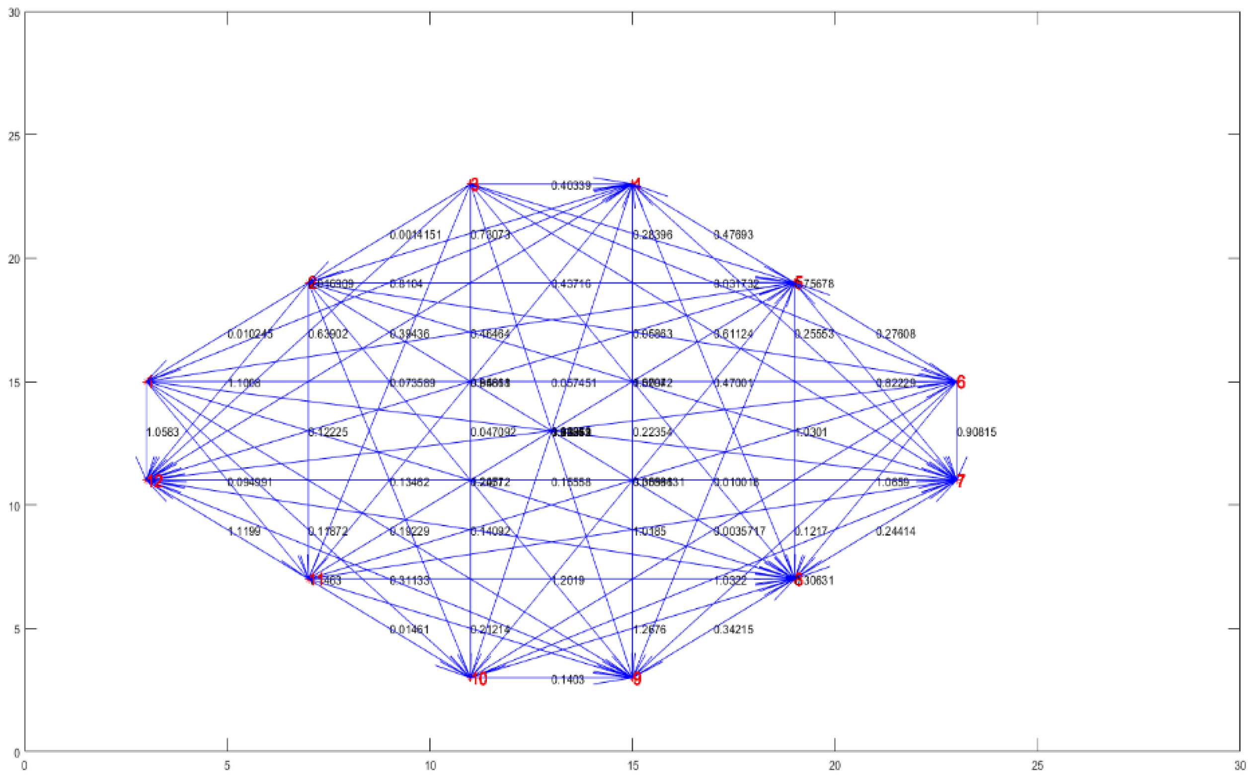2000 groups of data are selected as samples to construct the initial FTTas shown in Figure 8. The adjacency matrix between variables is shown in A₁. 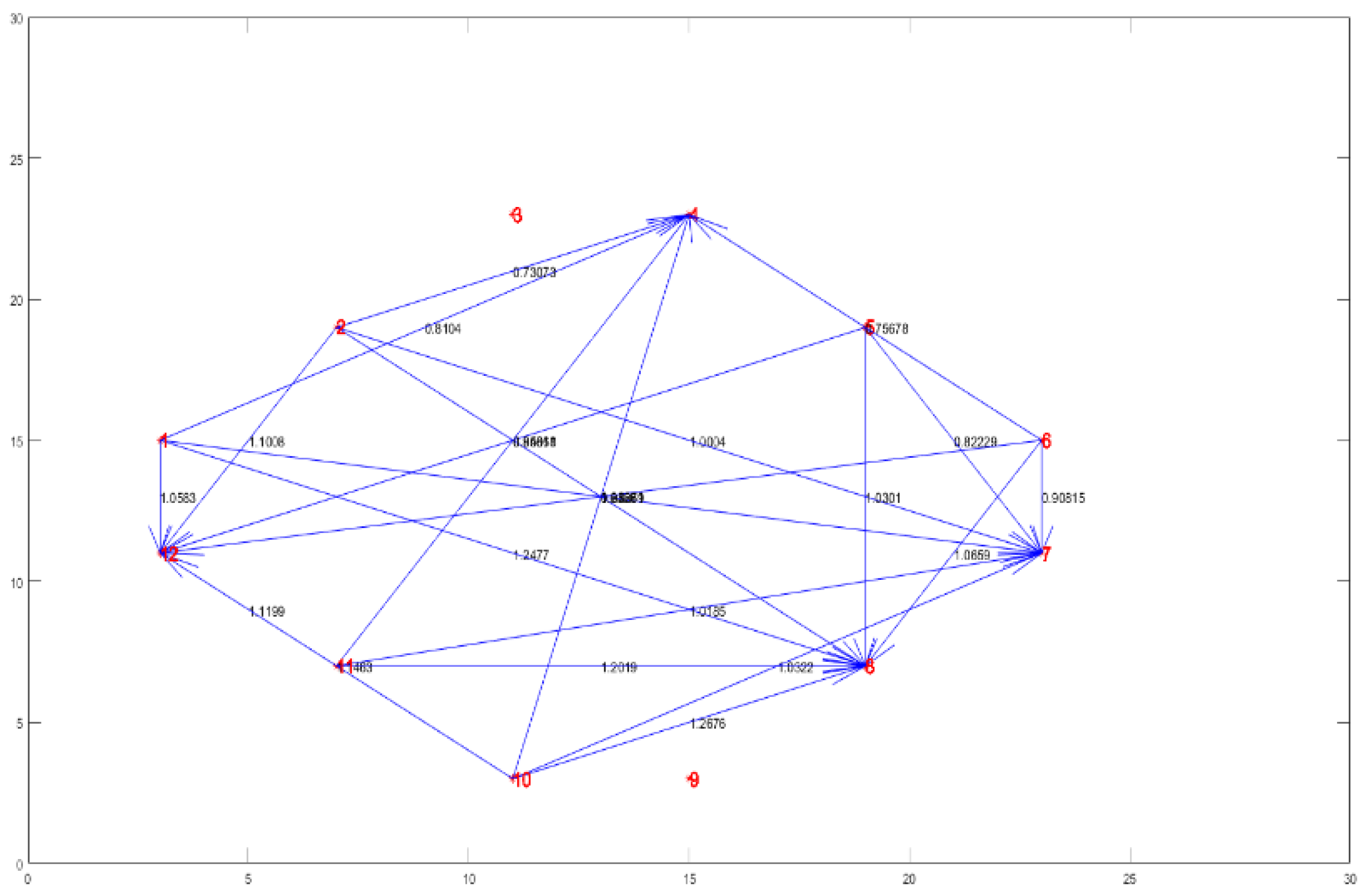It can be found from Figure 8 that the FTT has high complexity, so it is necessary to extract stronger causality. The FTT can be simplified by setting a threshold value. The adjacency matrix between variables is shown in A₂. As shown in Figure 9, the simplified FTT is obtained, which can represent the relationship between fault variables.

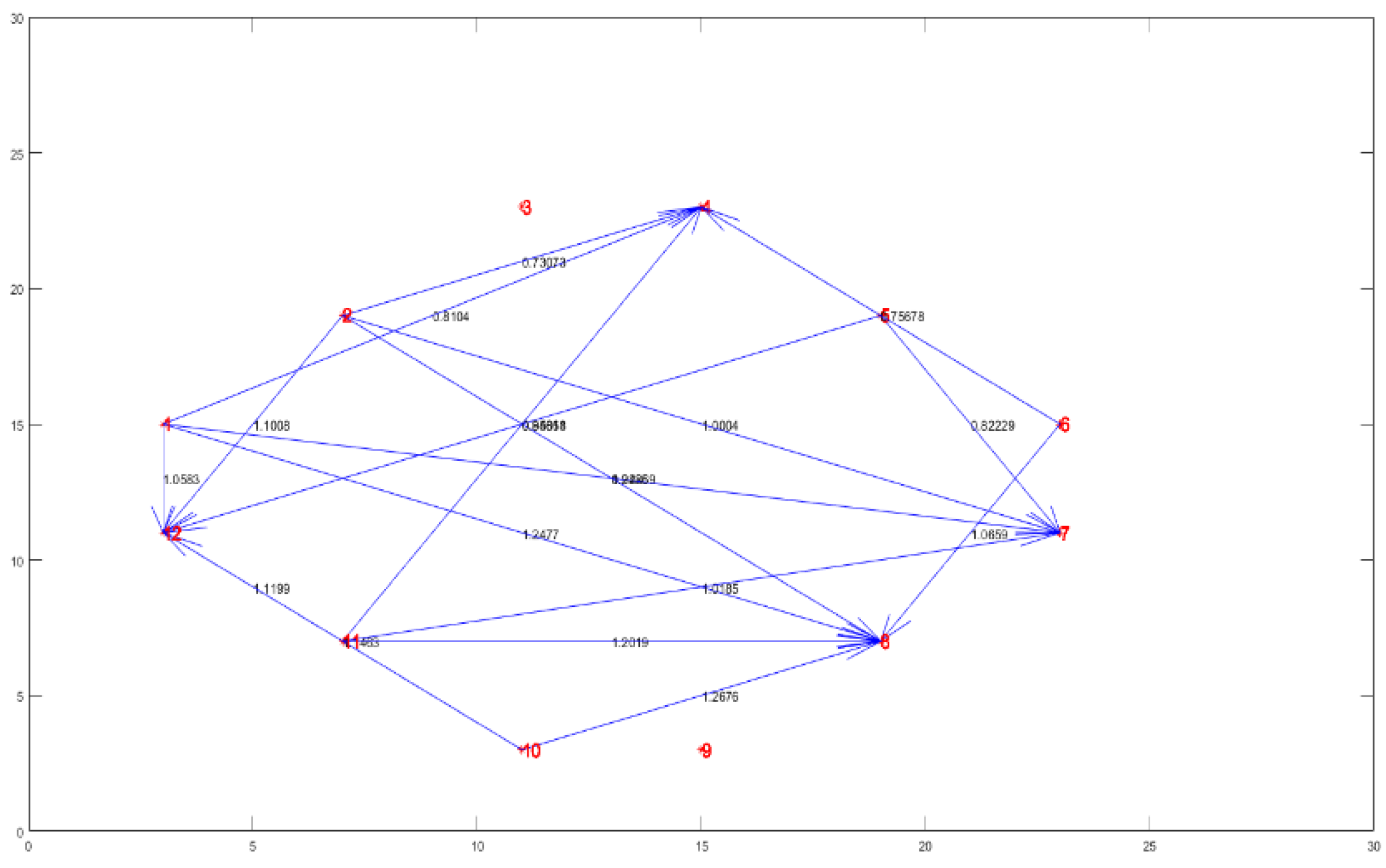
As shown in Figure 10, the information compressible strategy is used to further simplify the fault transfer topology. The adjacency matrix between the variables is shown in A₃. In this experiment, the root causal variables of membrane fouling are diagnosed according to the simplified fault transfer topology, and the effectiveness of CDM is compared with other diagnosis methods.

$$A_3=\left(\begin{array}{c}\begin{array}{rrrrrrrrrrrr}\hfill 0& \hfill 0& \hfill 0& \hfill 0.810403& \hfill 0& \hfill 0& \hfill 0.942594& \hfill 1.247714& \hfill 0& \hfill 0& \hfill 0& \hfill 1.058295\\ \hfill 0& \hfill 0& \hfill 0& \hfill 0.730733& \hfill 0& \hfill 0& \hfill 1.000398& \hfill 1.228595& \hfill 0& \hfill 0& \hfill 0& \hfill 1.100775\\ \hfill 0& \hfill 0& \hfill 0& \hfill 0& \hfill 0& \hfill 0& \hfill 0& \hfill 0& \hfill 0& \hfill 0& \hfill 0& \hfill 0\\ \hfill 0& \hfill 0& \hfill 0& \hfill 0& \hfill 0& \hfill 0& \hfill 0& \hfill 0& \hfill 0& \hfill 0& \hfill 0& \hfill 0\\ \hfill 0& \hfill 0& \hfill 0& \hfill 0& \hfill 0& \hfill 0& \hfill 0.822288& \hfill 0& \hfill 0& \hfill 0& \hfill 0& \hfill 0.958113\\ \hfill 0& \hfill 0& \hfill 0& \hfill 0.756785& \hfill 0& \hfill 0& \hfill 0& \hfill 1.065932& \hfill 0& \hfill 0& \hfill 0& \hfill 0\\ \hfill 0& \hfill 0& \hfill 0& \hfill 0& \hfill 0& \hfill 0& \hfill 0& \hfill 0& \hfill 0& \hfill 0& \hfill 0& \hfill 0\\ \hfill 0& \hfill 0& \hfill 0& \hfill 0& \hfill 0& \hfill 0& \hfill 0& \hfill 0& \hfill 0& \hfill 0& \hfill 0& \hfill 0\\ \hfill 0& \hfill 0& \hfill 0& \hfill 0& \hfill 0& \hfill 0& \hfill 0& \hfill 0& \hfill 0& \hfill 0& \hfill 0& \hfill 0\\ \hfill 0& \hfill 0& \hfill 0& \hfill 0& \hfill 0& \hfill 0& \hfill 0& \hfill 1.267596& \hfill 0& \hfill 0& \hfill 0& \hfill 1.146267\\ \hfill 0& \hfill 0& \hfill 0& \hfill 0.846681& \hfill 0& \hfill 0& \hfill 1.018529& \hfill 1.201856& \hfill 0& \hfill 0& \hfill 0& \hfill 1.119884\\ \hfill 0& \hfill 0& \hfill 0& \hfill 0& \hfill 0& \hfill 0& \hfill 0& \hfill 0& \hfill 0& \hfill 0& \hfill 0& \hfill 0\end{array}\end{array}\right)$$

(19)

To evaluate the diagnostic efficiency of fault transfer topology (FTT) with an information compressible strategy (ICS) and a threshold, the results were compared with some other methods: FTT with threshold, initial FTT, Bayesian network (BN), ANN, and fuzzy logic (FL). The comparison results of FTT with ICS and a threshold to other methods are involved with diagnosis time, number of connections, and accuracy. In Table 2, it can be seen that the proposed FTT with ICS and a threshold achieves the least number of connections compared to FTT without ICS or a threshold. It means that the designed ICS and threshold can simplify the failover topology which also contributes to speeding the diagnosis of membrane fouling. In addition, the accuracy of FTT with ICS and a threshold is also best compared to other methods, which indicates that the proposed FFT in CDM is in favor of exploring the root causal variables of membrane fouling.

D. Analysis of Experimental Results

Based on the above experimental results and analysis, the performance of CDM is significantly superior to other existing methods. The main merits of CDM are summarized as follows.

1) Good detection. It is essential for CDM to identify incidents of membrane fouling with specific causal variables. The proposed autoencoder can summarize thresholds by RMSE for any membrane fouling, assuming it covers the entire normal conditions of MBR. These thresholds can serve as a reference for operators to monitor the occurrence of membrane fouling without the need of a physical or mathematical model. The results in Figs 6-7 also illustrate the efficacy of this method.

2) Intuitive diagnosis. By constructing fault transfer topology with CDM in Figure 8, the dynamic observation of causal relationships between variables facilitates the determination of causal factors leading to membrane fouling. Additionally, to eliminate repetitive affiliation relationships, the fault transfer topology is simplified using an information compressible strategy, as shown in Figs. 9-10. Table 2 also demonstrates that the proposed CDM significantly enhances the speed and accuracy of diagnosis.

5. Conclusions

Membrane fouling is a bottleneck problem to the wide application of MBR. A CDM is proposed, which can diagnose the root causal variables of membrane fouling and improve the diagnosis accuracy. Firstly, the causal relationship between variables is judged based on the transfer entropy to obtain the initial fault transfer topology. Then, the typical causal relationship of variables is extracted based on the significance threshold to obtain the simplified fault transfer topology. For each feasible structure, the fitting degree between data structures and the complexity of the structure are comprehensively considered through the information compressible strategy. The fault transfer topology can be simplified to improve the diagnosis accuracy. The experimental results show that this compressible diagnosis model can accurately diagnose membrane fouling, which is significant for decision-making of membrane fouling. Future research will focus on investigating its generalizability to different MBR systems and other membrane-based processes.