Preprint
Article

Fourier Features and Machine Learning for the Contour Profile Inspection in CNC Milling Parts: A Novel Intelligent Inspection Method (NIIM)

Altmetrics

Downloads

116

Views

43

Comments

0

A peer-reviewed article of this preprint also exists.

Submitted:

09 August 2024

Posted:

12 August 2024

You are already at the latest version

Alerts
Abstract
Form deviation generated during the milling profile process poses challenges to the precision and functionality of industrial fixtures and product manufacturing across various sectors. The inspection of contour profile quality often relies on commonly employed contact methods for measuring form deviation, but these methods frequently face limitations that can impact the reliability and overall accuracy of the inspection process. This paper introduces a novel approach, the novel intelligent inspection method (NIIM), developed to accurately inspect and categorize contour profiles in machined parts manufactured through the milling process by computer numerical control (CNC) machines. The NIIM integrates a calibration piece, a vision system (RAM−StarliteTM), and machine learning techniques to analyze the line profile and classify the quality of contour profile deformation generated during CNC milling. The calibration piece is specifically designed to identify form deviations in the contour profile during the milling process. The RAM−StarliteTM vision system captures contour profile images corresponding to curves, lines, and slopes. An algorithm generates a profile signature, extracting Fourier descriptor features from the contour profile to analyze form deviations when compared to an image reference. A feed-forward neural network is employed to classify contour profiles based on quality properties. Experimental evaluations involving 60 machined calibration pieces, resulting in 356 images for training and testing, demonstrate the accuracy and computational efficiency of the proposed NIIM for profile line tolerance inspection. Results demonstrate that the NIIM offers 96.99% accuracy, low computational requirements, 100% inspection capability, quality classification.
Keywords: 
Subject: Computer Science and Mathematics  -   Computer Vision and Graphics

1. Introduction

The quality of contour profiles plays a crucial role in the functionality of fixtures and assembly parts in manufacturing products across various applications, including automotive, aerospace, and household appliances [1]. The fixture assumes a pivotal role by precisely positioning components, directly impacting both product quality and the successful execution of computer numerical control (CNC) processes. The industry’s rapid adoption of smart CNC has prompted the development of stringent geometric tolerance standards for CNC milling parts, leading to rigorous inspection protocols designed to optimize functionality [2]. These protocols could include some diagnostic technologies, including automated visual inspection (AVI), X-ray inspection, thermographic inspection, ultrasonic inspection, and laser inspection. In some instances, conducting a thorough inspection can be quite expensive. Tool wear analysis is essential for maximizing cutting tool life and preventing errors in CNC processes [3,4]. Chatter, characterized by vibrations at the tool-workpiece interface, induces excessive cutting forces [5], tool damage, and higher removal rates [6]. Numerous studies delve into predicting form deviations caused by tool wear and chatter detection. For instance, [7] and [8] posit that milling processes can generate form deviation, impacting the quality and functionality of machined parts. Myshkin et al. [9] stress the importance of characterizing form deviation using statistical parameters derived from surface profiles or 3D surface maps. Cheung and Bun [10] highlight the contributions of various components, such as tool feed rate, spindle rotational speed, tool geometry, material properties, and tool-work vibration, to the generation of profile deformation and resulting surface modulation variations. Prabhakar et al. [11] outline common instruments for measuring contour profiles, including coordinate measuring machines (CMMs), optical profilometers, and 3D scanners. The choice of common instruments depends on specific measurement task requirements, such as precision, surface type, and contour profile complexity. While common instruments excel in measuring profile contour with excellent accuracy, they have limitations, including time-consuming measurements, stylus wear, and the potential for scratches on finished part surfaces. Conversely, non-contact methods, particularly those involving computer vision and machine learning, present innovative solutions for efficiently measuring and assessing form deviation. For instance, the study by Kochetkov et al. [12] underscores the transformative advancement of non-contact methods in contour profile inspection, offering benefits such as speed, accuracy, efficiency, and adaptability to complex geometries. In a similar vein, [13] utilize multilayer perceptron (MLP) and 2-D convolutional neural network (CNN) models to classify surface profiles with an average accuracy rate exceeding 99.6%. [14] harnesses pre-trained networks to classify and recommend cutting conditions, with an effectiveness rate of 99.4%.
According to the state-of-the-art presented in [15] and [16], the most common methods for preprocessing and feature extraction are principal component analysis (PCA), variational mode decomposition (VMD), empirical mode decomposition (EMD), Wavelet transform (WT), and Fourier transform (FT). The most common classification methods are support vector machines (SVM) because of their feasibility implementation in lineal classification, convolutional neural networks (CNN) because they can find abstract features, and recurrent neural networks (RNN). After all, they can find patterns in time series and historical information on profile deviation, texture, tool wear, or chatter features.
Various methods have been proposed for measuring contour profiles using signal processing and computer vision algorithms. Ali et al. [17] developed an algorithm using higher-order Wavelet transform coefficients to evaluate the form deviation in electric discharge machine (EDM) machining. Ketaki and Bhushan[18] and Sepehr and Masoud[19] developed other approaches for surface roughness evaluation involving the utilization of histograms, gray-level co-occurrence matrices, Fourier and Wavelet transforms, and neural networks. The works in [20,21,22] developed applications of Fourier-invariant moments and descriptors in geometric and profile property inspection, image retrieval, and object recognition. In addition, [23] and [24] utilized Fourier descriptors for dimensional inspection, shape classification, and form deviation evaluation in machining processes. However, developing a system that tries to monitor form deviation, tool wear, and chatter with real-time processing and accurate methodology is necessary. Also, fixture design in CNC milling processes is crucial because it directly impacts various facets of the manufacturing workflow. Fixtures are the foundation for securing and positioning workpieces during milling operations, which ensures precision, repeatability, and efficiency.
Based on these principles, the novel intelligent inspection method (NIIM) is proposed to inspect the contour profile quality of machined parts. NIIM comprises a calibration piece, a vision system, and a machine learning method that analyzes the shape and quality of the contour profile deformation generated by the CNC machined process. The calibration piece is a machined part designed to find the contour profile deformation generated during the milling process with a profile composed of curve, line, and curve shapes. The vision system is a machine that captures three images, one for each shape of the calibration piece. The images are processed with a machine-learning method that employs Fourier descriptors and a feed-forward neural network (FFNN) that analyzes the form deviations to classify the quality of the shape deformation generated during the CNC milling process. For the experiments, 60 calibration pieces were machined to obtain a dataset of 356 images for training and testing.
The rest of the paper is organized as follows. Section 2 describes the methodology based on the vision inspection system and machine learning method. Section 3 explains the experimental setup, which consists of the machined process. Section 4 reports the results. Finally, Section 6 presents the conclusions.

2. Materials and Methods

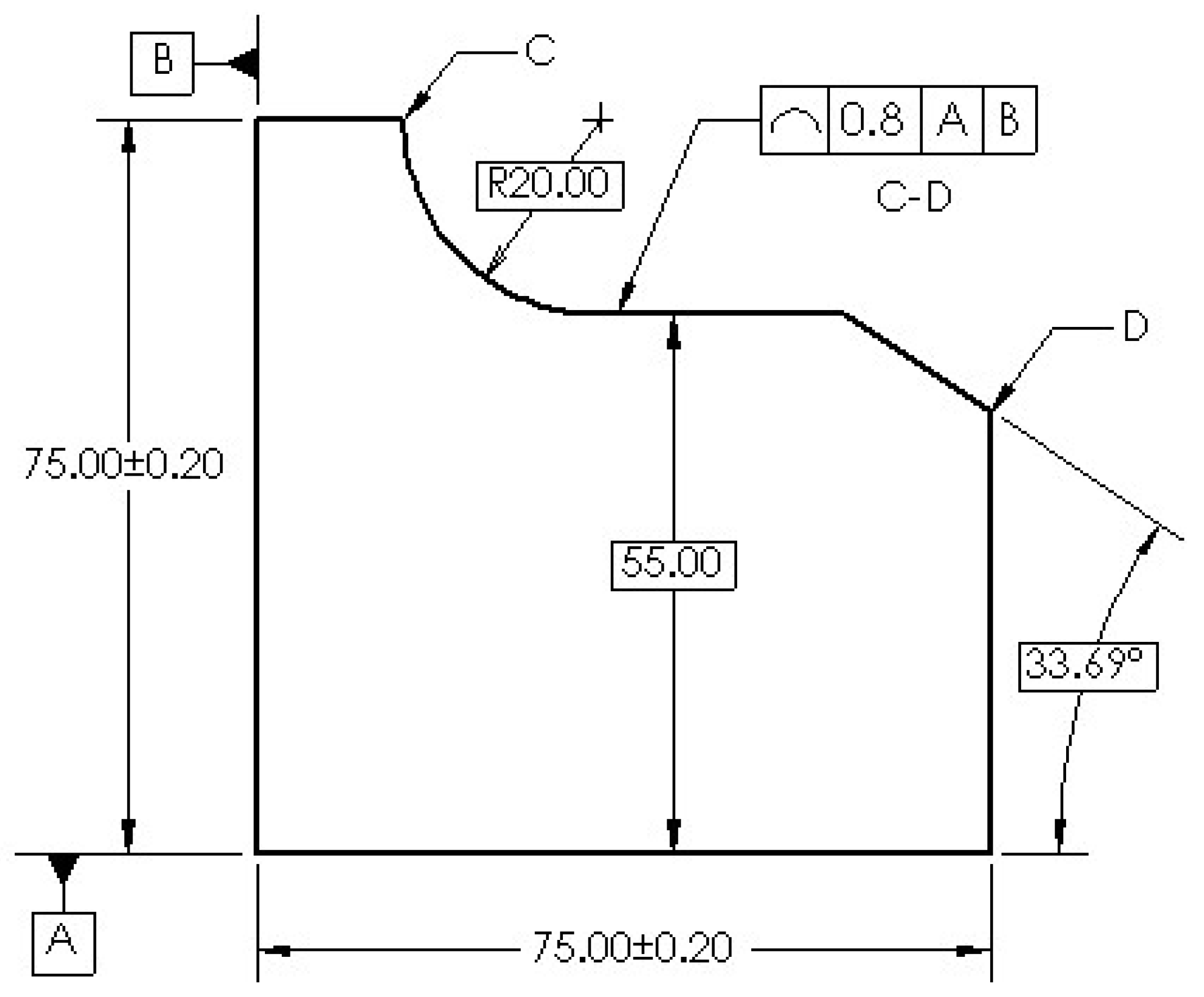
Aiming to inspect and classify the contour profile of CNC-machined parts using the NIIM, a calibration piece has been designed. Its purpose is to inspect the form deviation presented in a curve, line, and slope along the contour profile from C to D for each cross-section within a 0.8 profile of a line tolerance referenced to datums A and B, as depicted in Figure 1. This design is based on the standards outlined by ASME Y14.5 [25] and ISO 1101 [26], which provide the framework for precisely inspecting the individual contour profile.
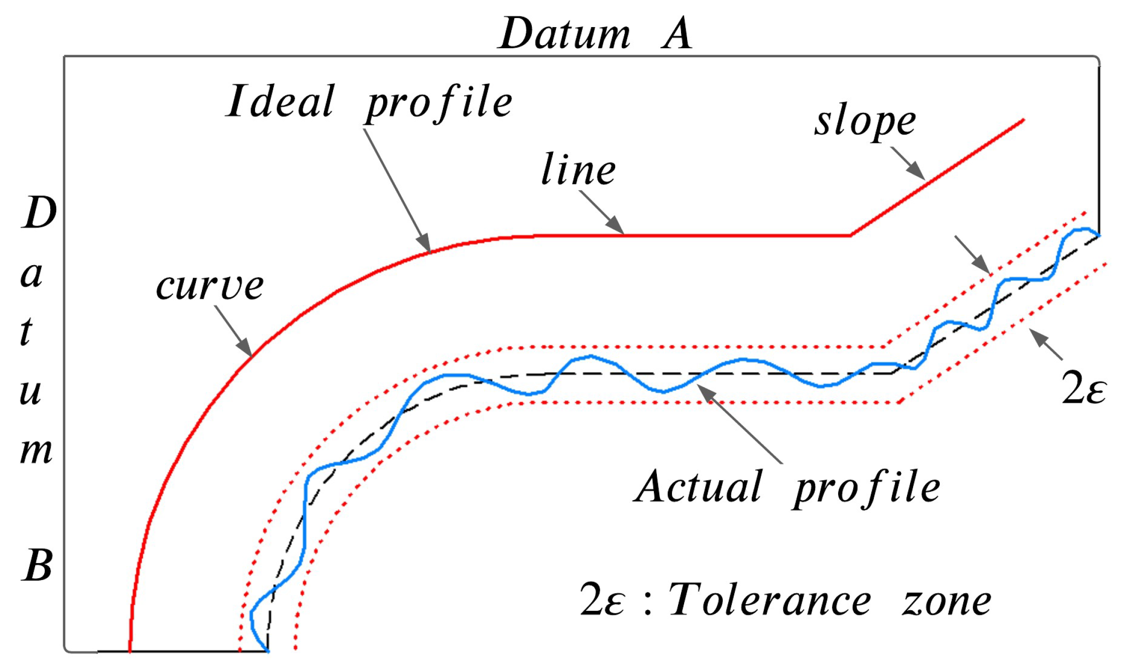
According to ASME Y14.5 [25] and ISO 8015:2011 standards, the tolerance zone for the profile of a line tolerance extends between points C and D at any given cross-section (not the entire surface). Figure 2 shows that the tolerance zone is distributed bilaterally concerning the true profile. The contour profile from C to D must lie between two profile boundaries 2 ε = 0.8 apart, referencing by datums planes A and B. Then, the form deviations presented in the contour profile must lie within the specified size limits for acceptable tolerance.
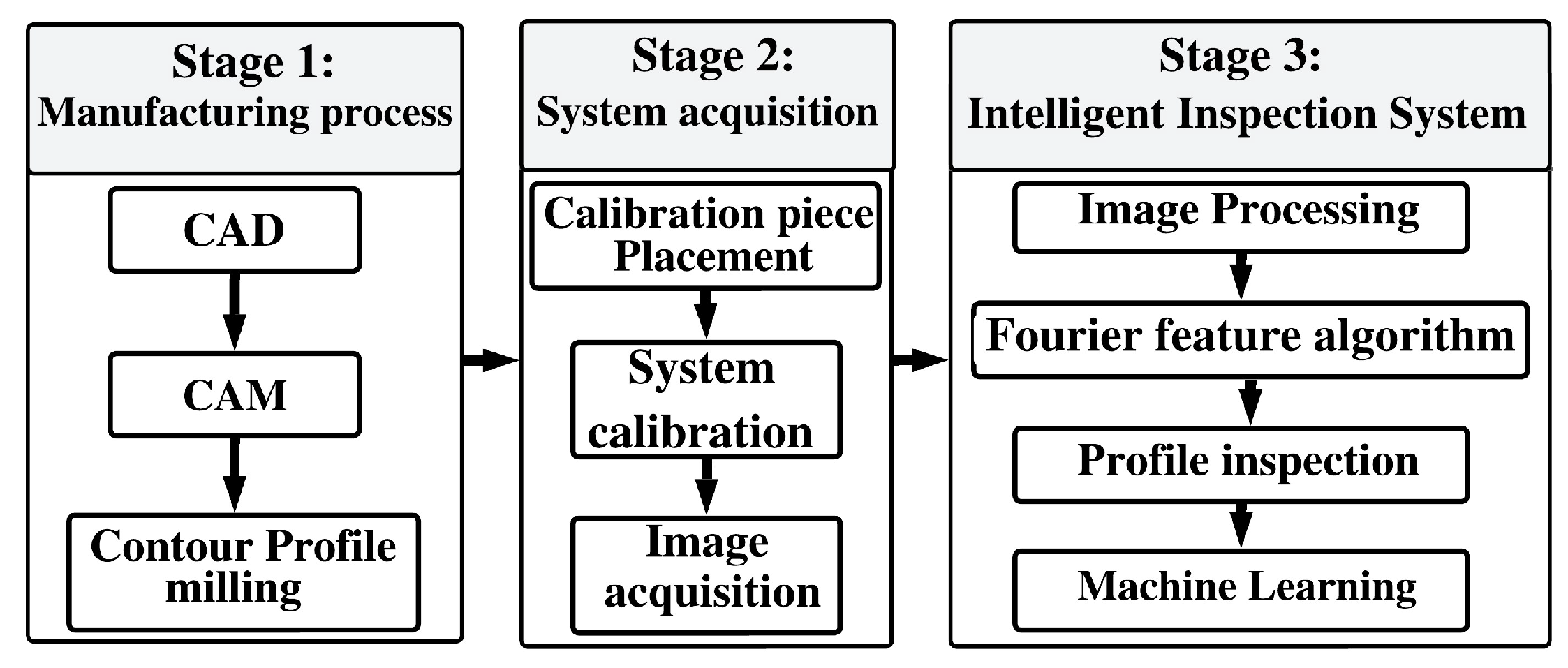
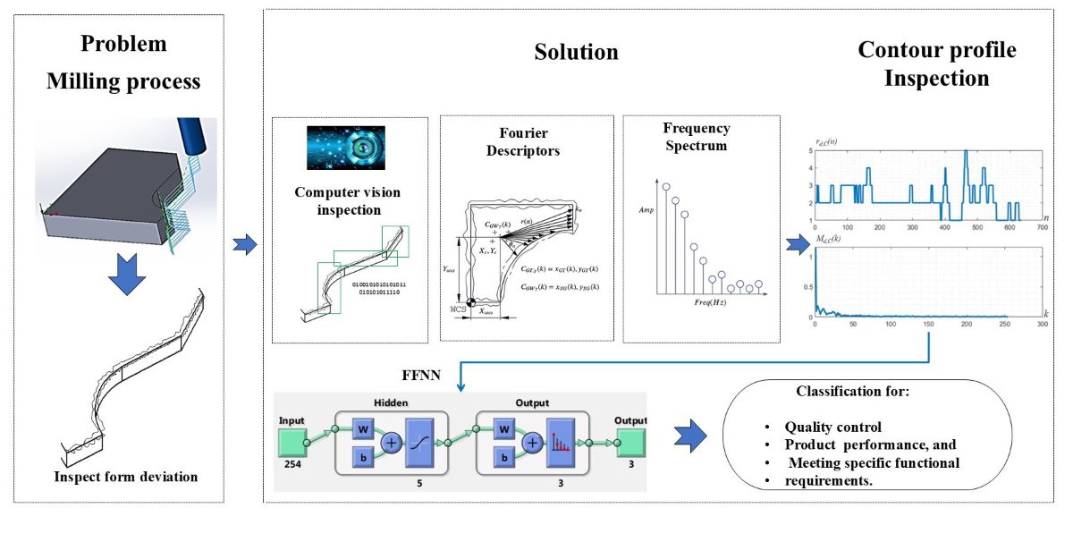
Figure 3 presents the methodology of the NIIM, which is divided into three stages: i) the manufacturing process, ii) the system acquisition, and iii) the intelligent inspection system. The manufacturing process stage includes computer-aided design (CAD), computer-aided manufacturing (CAM), and the CNC milling process to design and machine the profile of the calibration pieces. The system acquisition stage includes the calibration piece placement process, system calibration, and the image acquisition process to mount the calibration pieces, compute the positions, calibrate the camera, and capture the three images for each calibration piece: one for curve, one for line, and one for slope. Finally, the intelligent inspection system performs image processing, analyzes the form deviations with the Fourier features algorithm, and classifies the profile contour in defective and non-defective quality employing an artificial neural network (ANN). The following subsections explain the stages of the NIIM´s method.

2.1. Manufacturing process

The manufacturing process comprises the CAD, CAM, and milling process to design, simulate, and manufacture the contour profile of the calibration pieces.

2.1.1. CAD

The calibration piece design was conducted using CAD software, considering the contour profile and dimensions depicted in Figure 1. The contour profile is composed of a curve, defined as a quarter of a circle with a radius of 20 mm, a horizontal line with a length of 25 mm, and a slope represented by a line segment with a length of 12.5 mm inclined at an angle of 33 . 69 o . The contour profile was designed to be contended in a 75 × 75 × 12 mm rectangular workpiece within a line profile tolerance of 0.8 mm to obtain the ideal profile shown in Figure 2. The definition of the calibration piece guarantees the accuracy and relevance required for the NIIM to inspect the contour profiles, facilitating a thorough assessment of the machining processes.
Material selection was guided by optical and contrast properties, considering delrin (black), nylon (white), aluminum (silver), and AISI 1018 (gray) due to their interaction with light and impact on image acquisition quality [27]. Additionally, the choice aligns with findings from [28], highlighting these materials as commonly used in industrial applications. Refer to Table 1 for detailed properties.

2.1.2. CAM

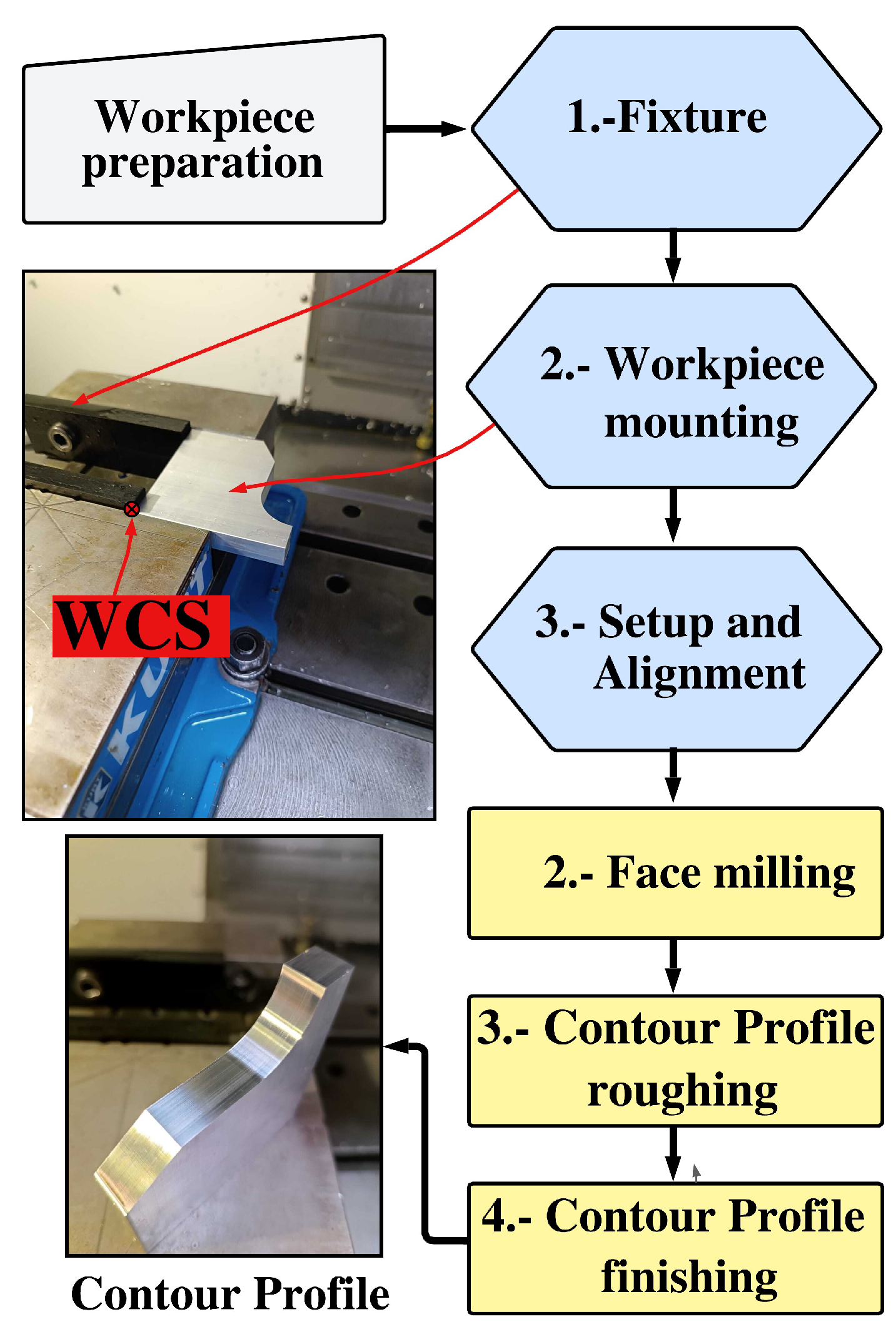
The CAM process was designed to generate the desired contour profile to inspect form deviation resulting from CNC milling processes. The CAM process considers tool-material compatibility and the sequence of operations shown in Figure 4.
The experimental machining conditions comprise the choice of materials, cutting tools, machining parameters, and the operations sequence. The selection of cutting tools is detailed in Table 2 and the machining parameters in Table 3. The tools were selected using the cutting theory proposed by George et al. [29] to find the optimal performance and efficiency in machining to generate contour profiles for inspection and classification.

2.1.3. Contour Profile Milling

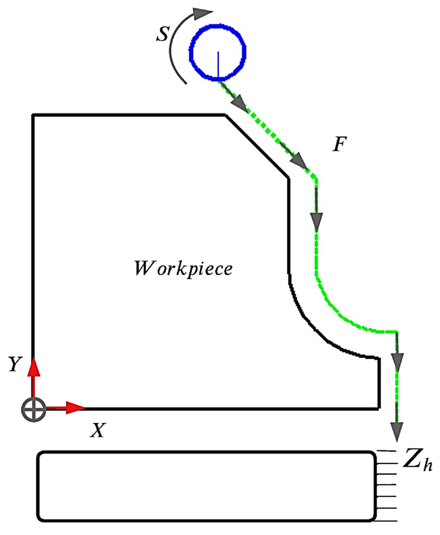
The CNC contour profile milling process was executed on a Haas VF1 three-axis vertical machining center, following the tool path outlined in Figure 5. The workpiece was securely affixed to the milling fixture, maintaining a 30 mm overhang distance from the milling vice. The sequential machining operations are detailed below:
  • The face milling operation was performed using a 16 mm coated solid carbide end mill, removing a depth of 1.5 mm from the workpiece.
  • A 12 mm coated solid carbide end mill performed a contour profile roughing operation, penetrating 1.5 mm each cut depth along the Zh axis until the total machined level was reached, leaving a 0.5 mm wall stock for finishing.
  • Contour profile finishing was performed utilizing a 9.52 mm coated solid carbide end mill to remove burrs and surface flaws. The cutting depth followed the same direction as the previous machining but with an increased cutting speed and a decreased feed rate.

2.2. System Acquisition

After machining the calibration pieces, the next stage encompasses the acquisition system process essential for capturing high-quality images, conducting contour profile inspections, and facilitating classification. The process is structured into three layers: calibration piece placement, system calibration, and image acquisition.
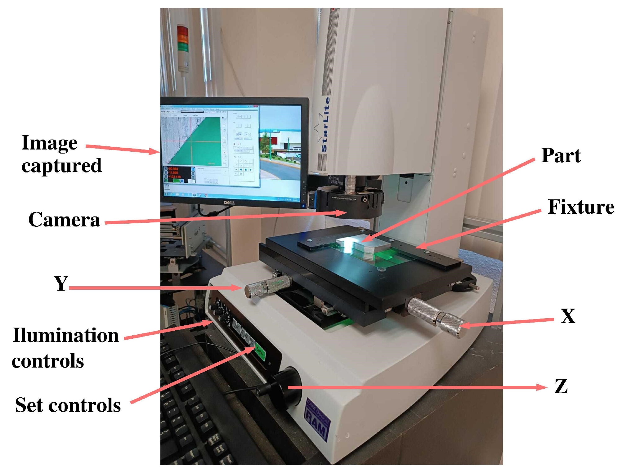
The employed acquisition system consists of a vision machine called R A M S t a r l i t e T M 150 shown in Figure 6. The R A M S t a r l i t e T M 150 machine captures the calibration piece profile in RGB images format designated as I α , β ( x , y ) R G B .
In the proposal, α takes on the value of either data (d) or ground truth (g), corresponding to the image profile. Meanwhile, β represents the profile of the image, with β encompassing L (line), S (slope), and C (curve). The image was acquired in the . b m p format within the RGB color space and a spatial resolution of 480 x 680 .
The selection of the R A M S t a r l i t e T M 150 system stems from its notable features to control the optimal parameters for image acquisition and provide the minimum resolution required for the experiment. The system boasts a maximum resolution distance of 62 mm and a dynamic field of view from 9.1 mm (low magnification) to 0.6 mm (high magnification), ensuring the capture of all relevant areas with precision and clarity.
System acquisition is essential for guaranteeing the quality of image capture [30], and its proper execution demands meticulous attention to the defined sequential steps, including calibration piece placement, system calibration, and image acquisition, as outlined in the following sections.

2.2.1. Calibration Piece Placement

Proper placement of the calibration piece in the R A M S t a r l i t e T M 150 is crucial for ensuring accurate image capture. As an initial step, a fixture mechanism has been introduced. Illustrated in Figure 7, the fixture, manufactured in 1020 Steel using CNC machining and grinding processes, aligns the calibration piece with specified datum references A and B. It effectively controls the orientation and location of profiles, ensuring stable and accurate positioning during image acquisition.

2.2.2. System Calibration

Following the placement of the calibration piece, the subsequent stage involves system calibration, a critical procedure. The system calibration process encompasses both camera calibration and the establishment of reference points, which are essential for positioning the precise profiles of the pieces within the visual field. The calibration ensures that the images acquired with the profile are properly aligned, facilitating comparison with ideal profiles referred to as ground truth (GT) I g , β ( x , y ) , as depicted in Figure 8.
In the system calibration process, crucial steps were undertaken to ensure the acquisition of image profiles with precise coordinates of GTs. The calibration procedure is interconnected and includes the following key points.
The first step involves camera calibration, encompassing adjusting parameters such as focal length, reference points, depth of field, white balance, lighting, and distortion coefficients (radial and tangential). Calibration is crucial to ensure the precision of image acquisition, especially considering the distinct material colors of aluminum, nylon, delrin, and steel 1018.
After camera calibration, the X and Y axes of the system are set to their respective home positions, establishing a consistent starting point for all subsequent movements and measurements within the system.
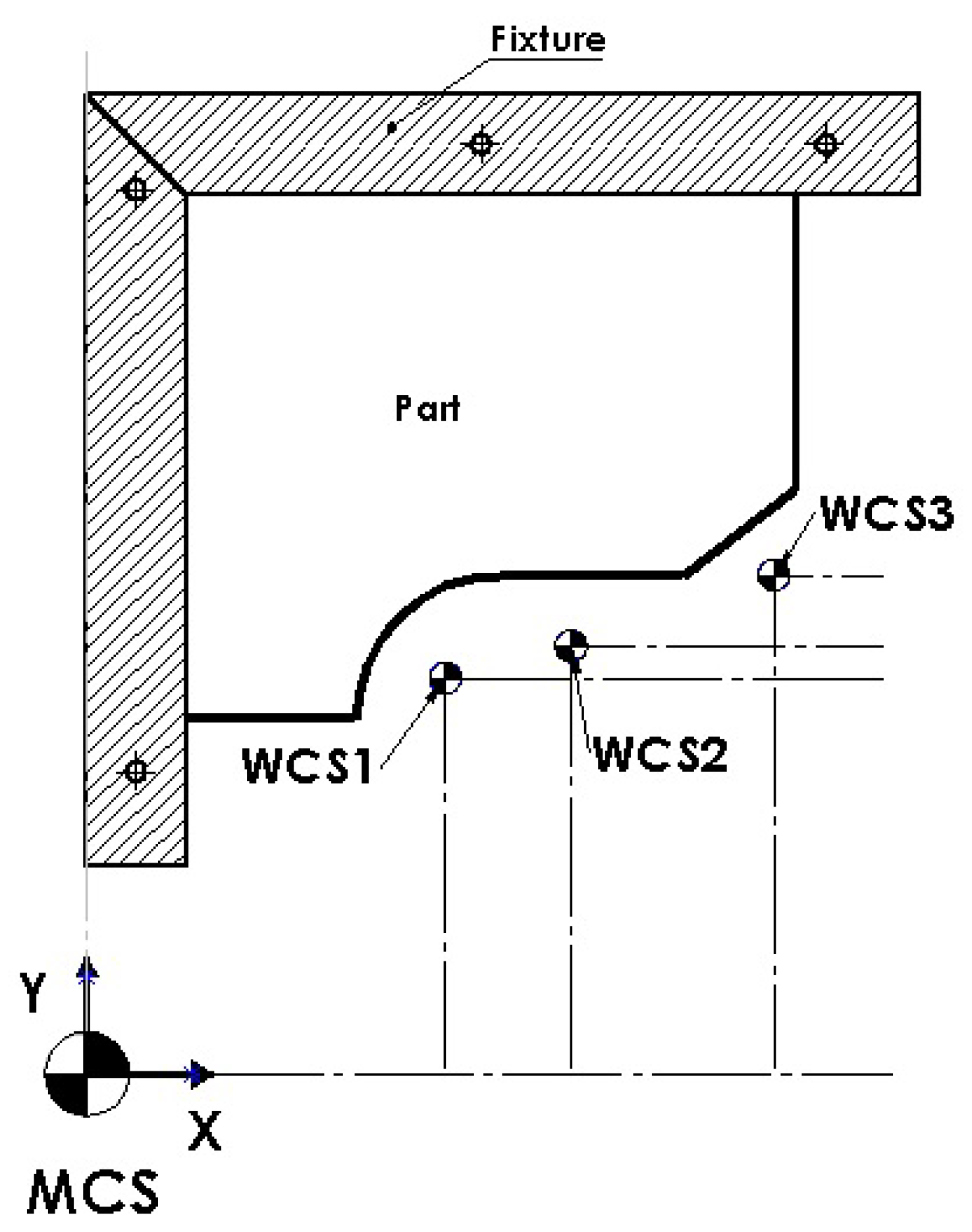
Further, each reference axis is set to a zero value, creating a baseline for positioning and measurement. Subsequently, the X and Y axes are moved to specific reference point positions defined by the WCS1, WCS2, and WCS3 coordinates established in Table 4, ensuring that the profiles align with the desired datum.
Lastly, the calibration data, including the camera’s intrinsic and distortion parameters, is saved for future use in all image analysis software. By interconnecting these steps, the camera calibration process ensures accurate and reliable image profiles for subsequent analysis.

2.2.3. Image Acquisition

After completing the system calibration, the vision system acquires three images for each piece: one for the curve profile, another for the line profile, and a third for the slope profile. Each image is denoted as I α , β ( x , y ) R G B . Figure 9 illustrates three images obtained from the black delrin calibration piece.

2.3. Intelligent Inspection System

The following subsections outline the functionality of the intelligent inspection system, which includes the stages of image processing, Fourier descriptors, profile analysis, and machine learning.

2.3.1. Image Processing

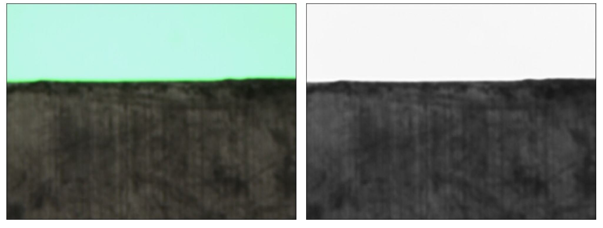
The color image I α , β ( x , y ) R G B generated by the acquisition system is processed and converted to the green channel I α , β ( x , y ) G for Machine Learning purposes. This conversion is based on our experiments with different color spaces, revealing that I α , β ( x , y ) G provides the best contrast between the calibration piece profile and the illumination of the vision system. Figure 10 illustrates an example of the conversion of I α , β ( x , y ) R G B .
The shape of the contour profile presented in I α , β ( x , y ) G is analyzed through a machine learning method composed of feature extraction and classification layers, which will be analyzed in the following subsections.

2.3.2. Fourier Feature Algorithm

According to [3] and [4], PCA is the most common method used in feature extraction in multivariate analysis. WT and FT require other statistical analyses like VMD or EMD to generate features. However, these feature extraction methods cannot be used in online real CNC monitoring and diagnosis. On the other hand, Fourier descriptors are a set of methods for feature extraction based on the FT used in many industrial applications because they generate a one-dimensional feature vector composed of a low number of elements [31]. Fourier descriptors generate results with similar precision as WT and other FT methods but with significantly low computational complexity in CNC monitoring and industrial applications[32,33]. Then, Fourier descriptors are the foundations for feature extraction for the NIIM.
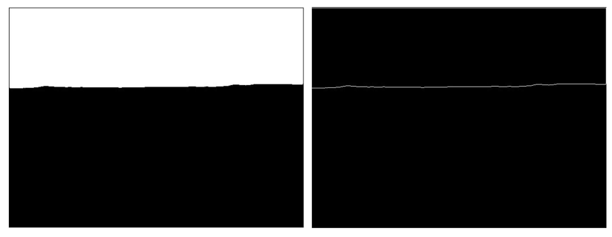
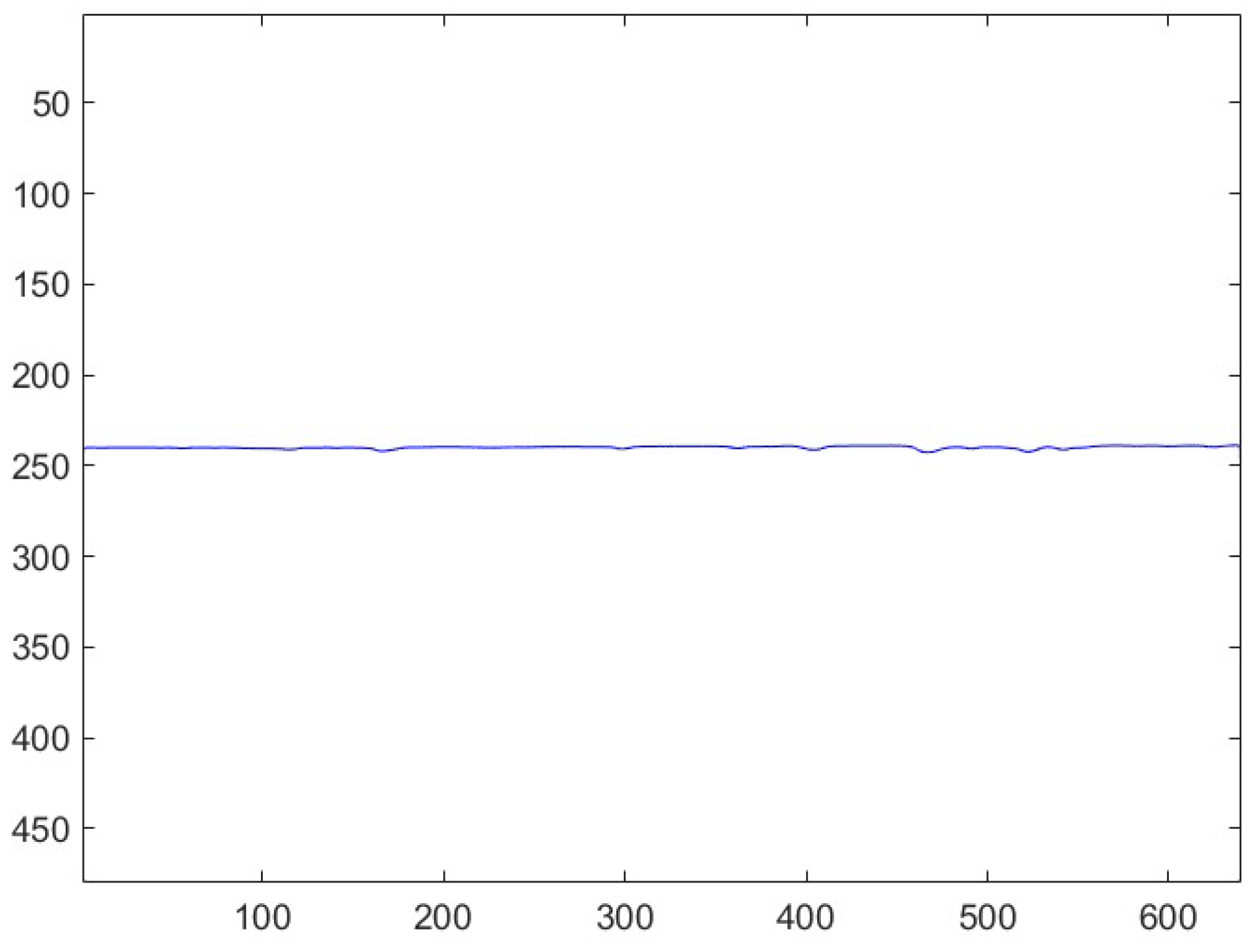
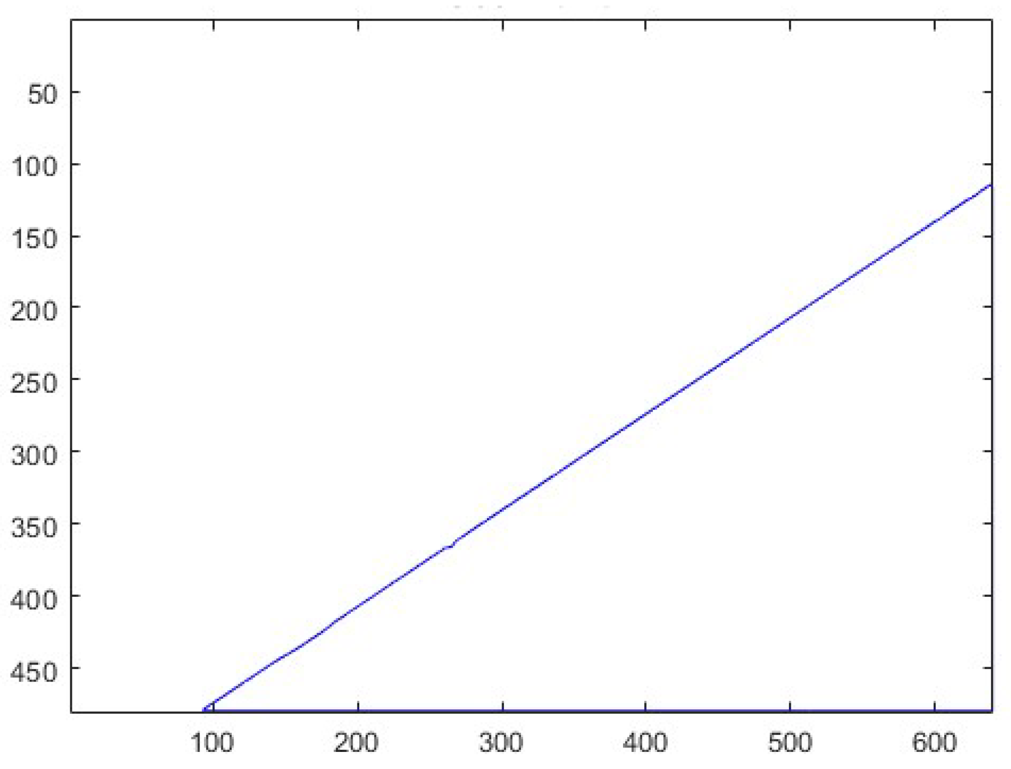
Subsequently, I α , β ( x , y ) G is segmented using the method of [34], generating an output B α , β ( x , y ) that divides the image into two regions: the piece and the illumination of the vision machine. The next step is to find the piece profile that computes the edge between the part and the illumination, defining P α , β ( x , y ) = B α , β ( x , y ) * h , where h = { 1 , 1 } . Next, P α , β ( x , y ) is scanned from left to right to determine the position ( x , y ) of pixels with values different from zero in P α , β ( x , y ) , as shown in Figure 11. This scanning generates a profile feature vector r α , β ( n ) defined by Equation 1.
r α , β ( n ) = x ( n ) 2 + y ( n ) 2
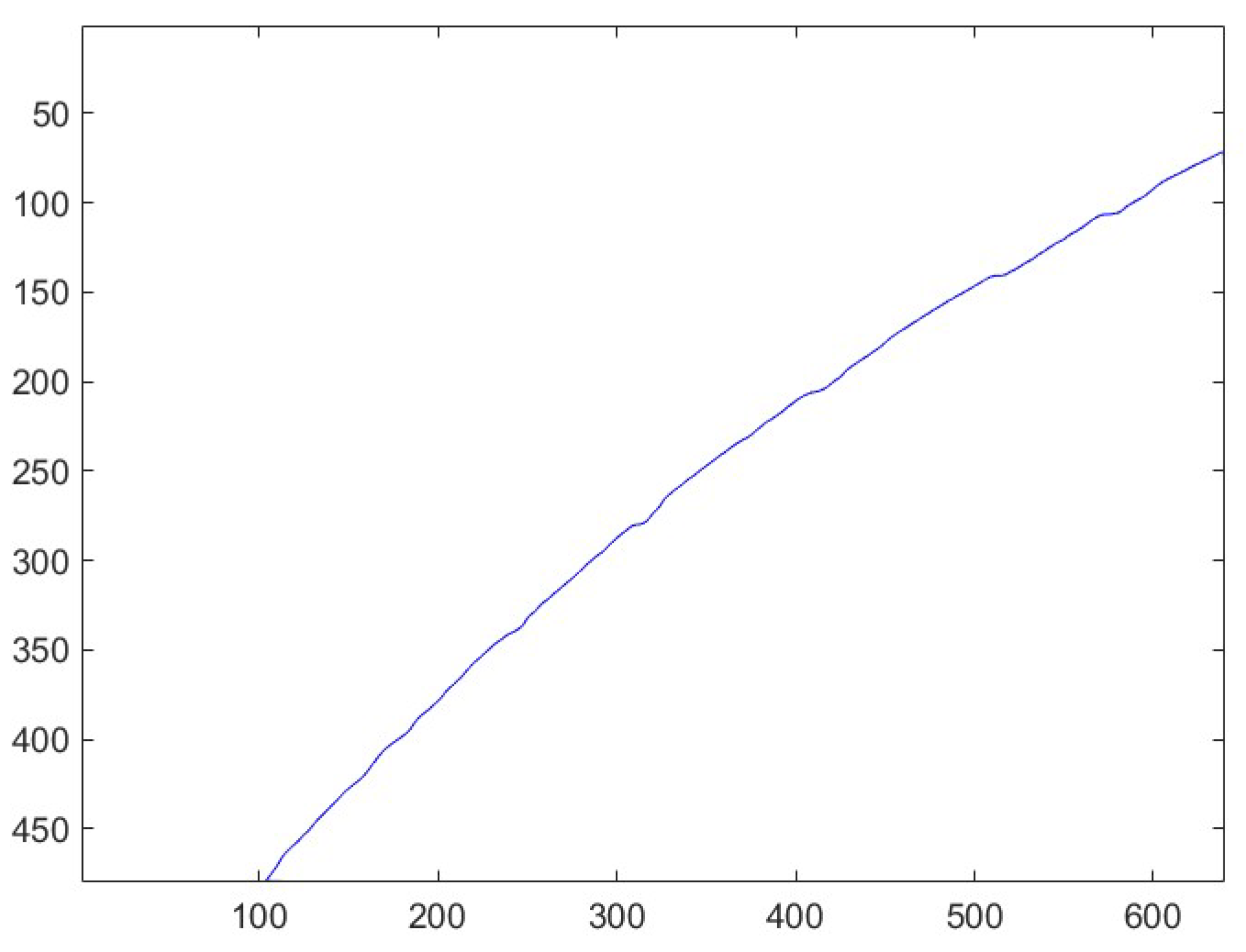
The contour profile feature vector r α , β ( n ) is converted into a signature I d , β ( x , y ) S G by the NIIM´s algorithm using the "Canny" function for edge detection proposed by [35]. The I d , β ( x , y ) S G allows extracting patterns, characteristics, and detailed information for analysis of the I d , β ( x , y ) S G intricacies, offering insights into the nuanced effects of the machining process on both shape and form.
The visual representations in Figure 12, Figure 13, and Figure 14 showcase how the signal r α , β ( n ) effectively highlights the form deviations within each I d , β ( x , y ) S G , providing a comprehensive understanding of the signature’s structural variations. The I d , β ( x , y ) S G analysis serves as a foundation for the subsequent implementation of the fast Fourier transform (FFT) to extract Fourier descriptors, enhancing the quantitative characterization of the I d , β ( x , y ) S G features. The subsequent step involves implementing the FFT to determine the Fourier Descriptors of r α , β ( n ) , as defined in Equation 2.
R α , β ( k ) = 1 N n = 0 N 1 r ( n ) α , β e x p j 2 π k n / N
where k is the frequency component, N is the size of the profile. Based on different works that apply Fourier descriptors in shape analysis as [33,34], the representation of the calibration piece profile Fourier features is defined by Equation 3 as the magnitude of Equation 2 divided by N.
M α , β ( k ) = R e ( R α , β ( k ) 2 + I m ( R α , β ( k ) 2 ) N
The profile feature vector M α , β ( k ) has the same shape and signature properties as r ( n ) , but these properties are described in the frequency domain. However, the profile feature is the Fourier spectrum Signature (FSS). The FSS describes the signature form properties and the concentration of the energy of the frequency components in M α , β ( k ) .
In contrast, the energy components derived from the form deviations caused by the machining process have little energy. However, the form deviations have features that describe the shape deformations and quality generated by the profile milling process. Therefore, the next step is to generate an FSS that accurately characterizes the profile deformation I d , β ( x , y ) S G in a frequency domain spectral analysis. The FSS provides valuable insights into the frequency components contributing to the observed form deviations, aiding in a comprehensive understanding of the machining process and facilitating informed improvements for enhanced precision and quality control.

2.3.3. Profile Inspection

The contour profile inspection is conducted by comparing the FSS between the GT reference I g , β ( x , y ) and the I d , β ( x , y ) S G . The comparison is achieved by subtracting the two FSS to obtain a third signal, which describes the variation in the form of the profile in terms of frequency. Finally, the energy is obtained to represent the microscopic distribution of peaks and valleys.
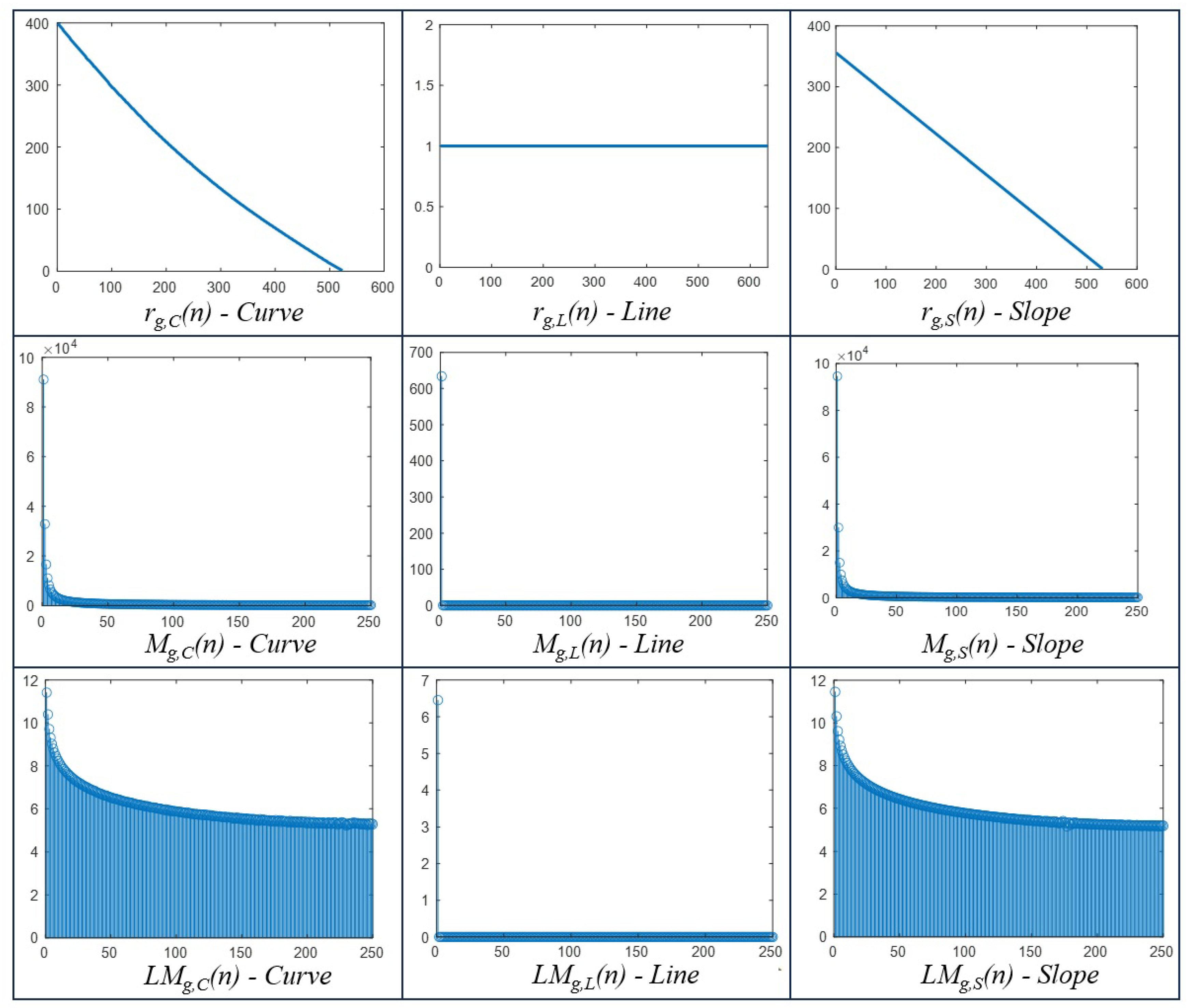
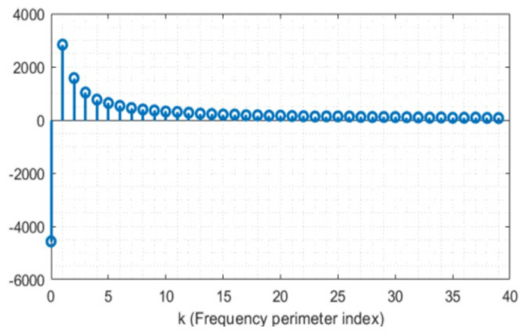
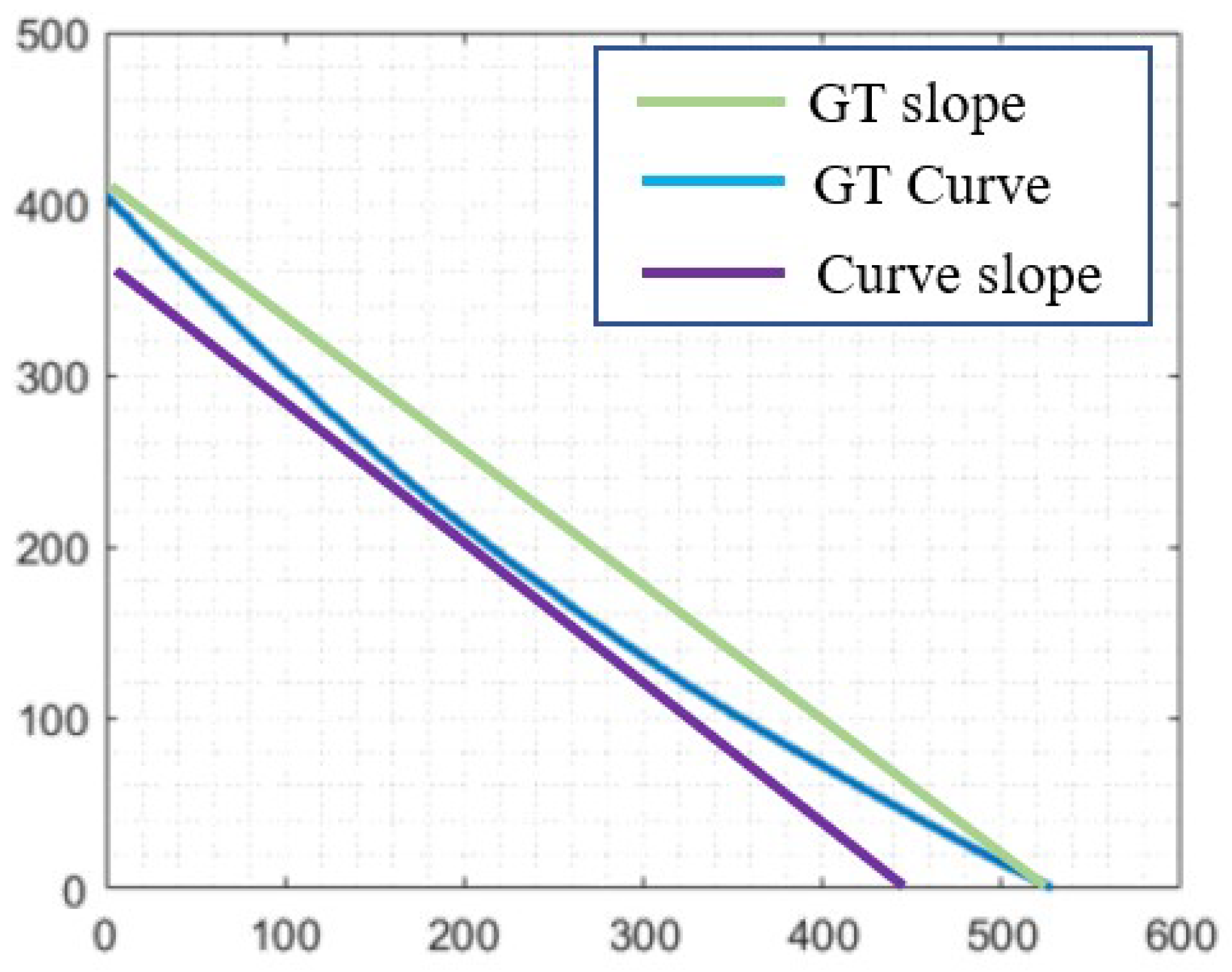
Figure 15 presents r g , β ( n ) , its M g , β ( k ) , and L M g , β ( k ) = L n ( M L g , β ( k ) + 1 ) of the GTs. As expected, the line profile generates frequencies with zero magnitudes except for M g , L ( 0 ) = 1 . The curve M g , C ( k ) and slope M g , S ( k ) generate frequencies with similar decreasing signatures. Nevertheless, there are differences in the magnitude frequencies that can be known with the difference of M δ ( k ) = M g , C ( k ) M g , S ( k ) . This difference is shown in Figure 16, where M δ ( 0 ) < 0 , M δ ( k ) with 0 < k < 40 have magnitudes higher than zero and M δ ( k ) 0 for k > 40 . This behavior occurs because the GT Curve is composed of a slope with less area than the GT slope and some frequencies that form the curve, as shown in Figure 17.
The Form deviation out of tolerance of the I d , β ( x , y ) S G is determined through the comparison of the FSS of the profile shapes with those of the I g , β ( x , y ) according to the profile of a line tolerance based in ASME Y14.4 [25] defined by Equation 4.
D Δ , β ( k ) = ( M d , β ( k ) M g , β ( k ) ) 2
where M d , β ( k ) are the Fourier features defined in Equation 3 of the I d , β ( x , y ) S G , which is used for the profile analysis. Each vector D Δ , β ( k ) comprises more than 300 frequency components, considering that the signatures consist of approximately 600 to 640 elements. Our experiments, guided by Fourier transform properties [11], have revealed distinctive features of D Δ , β ( k ) :
Frequency k = 0 is specifically associated with millimetric errors resulting from the calibration piece’s placement on the Fixture, primarily induced by profile shape deformations.
For frequencies 1 > k > 250 , these components describe form deviations from the machining process employed to generate a curve, a line, and a slope. Notably, frequencies within the 1 > k > 40 range offer a more detailed characterization of the shape induced by the machining process, providing valuable insights into the shape and quality of milling.
Similarly, frequencies 1 > k > 100 delineate quality errors in the calibration piece attributable to burrs, defects caused by tool wear, and errors occurring during machining. The interconnected analysis of these frequency components contributes to a comprehensive understanding of the calibration piece’s characteristics and manufacturing processes.

2.3.4. Machine Learning

The processing method for shape and quality profile classification is a feed-forward neural network (FFNN) composed of three layers: input, hidden, and output. The D Δ , β ( k ) , M d , β ( k ) , and r d , β ( n ) are a one-dimension and single-channel feature vectors that can be codified with an FFNN. The FFNN is a classifier less computationally complex than the classifiers most used in the literature related to CNC process monitoring. These classifiers are SVM, RNN, and CNN [15,16]. Also, the FFNNs learn with hundreds of feature vectors, while SVM, RNN, and CNN require tens of thousands of feature vectors to learn. Then, the shape and quality profile classification method is an FFNN composed of three layers: input, hidden, and output. The inputs are the features of the profile, F ( k ) . The hidden layer is composed of N neurons, defined by Equation 5.
γ 1 , j 1 = f ( ω 1 ( k ) F ( k ) + ω 1 , o )
where γ 1 , j is the hidden layer, ω 1 ( k ) are the weights, ω 1 , o are the bias, f ( · ) is the RELU activation function [36], and j 1 is the neuron index of the hidden layer, j 1 = 0 , . . . , J . The output layer is defined by Equation 6.
γ 2 , j 2 = f ( ω 2 ( k ) M Δ , β ( k ) + ω 2 , o )
where γ 2 , j 2 is the output layer, j 2 is the neuron index of the output layer, ω 2 ( k ) are the weights, ω 2 , o is the bias, and f ( · ) is the sigmoid activation function [37].

3. Experimental Setup

An experimental setup and methodology were designed to inspect and classify the contour profile of machined parts using the NIIM. The approach involves utilizing calibration pieces, employing an intelligent vision system, and implementing image processing alongside machine learning algorithms for proficient profile classification.
According to [3,4,6,15,16,38], a traditional machine learning approach requires dozens of milling parts to train and test ANNs for classification purposes in contour profile measurement applications. Subsequently, 60 pieces were machined as part of the experimental requirements, utilizing the Haas VF1 CNC machine detailed in Section 2.1. Within this set, 15 pieces were crafted from delrin, 15 from nylon, 15 from aluminum, and 15 from steel. An illustration of calibration pieces made from delrin, nylon, aluminum, and steel is depicted in Figure 18. The selection of the materials was specifically chosen to represent a diverse range commonly encountered in machining processes.

3.0.1. Image Dataset 

The machined pieces were used to generate a dataset for training and testing the proposed algorithms. The dataset is composed of 356 images in format I α , β ( x , y ) R G B , where 180 were generated with the 60 calibration pieces and the other 176 images were generated with the generative adversarial network of [39]. Table 5 presents the organization of the dataset developed for the NIIM, where the 356 images are balanced into 90 delrin images, 90 nylon images, 88 aluminum images, and 88 steel images. Regarding the shape, there are 120 curve images, 119 line images, and 118 slope images for the machine learning experiments.

3.0.2. Machine Learning Experiments 

The machine learning experiments were conducted on a laptop with a 2.60GHz i7-10750H CPU, 16 GB RAM, and an NVIDIA GeForce RTX 1650 Ti GPU. The experiments addressed two primary tasks: contour profile inspection and quality profile classification.
In the contour profile inspection, each image is classified into curve, line, or slope categories to ensure that the profile fixture or products adhere to specific interchangeable tolerances. It also helps identify deviations from the desired profile, detect potential production process issues, and provides documented evidence for quality control. The second task involves profile quality analysis, classifying contour profiles as normal or defective. The selection of the profile quality analysis task is motivated by findings in [40], which highlight the impact of contour profiles on assembly, shape deformation, tolerance accuracy, fatigue resistance, and fluid passage in fixtures.
The GTs used for the NIIM were designed by an expert geometric tolerance, dividing the dataset and considering geometric dimensions and tolerances according to ASME Y14.5.1M and ISO 1101-18 standards and quality standards for the automotive and household appliance industries. Various machine-learning methods, including different feature vectors and artificial neural networks (ANNs), were employed to implement profile inspection and quality classification. The objective was to identify machine-learning methods with optimal performance and computational efficiency for real-time applications in the industry.
The machine-learning methods considered are:
  • An FFNN named rFFNN where the input F ( k ) is x α , β ( n )
  • An FFNN named mFFNN where the input F ( k ) is M α , β ( k ) .
  • An FFNN named kFFNN where the input F ( k ) is D Δ , β ( k ) .
  • A convolutional neural network (CNN) named CNNG where is I α , β ( x , y ) R G B .
  • A CNN named CNNP where is P α , β ( x , y ) .
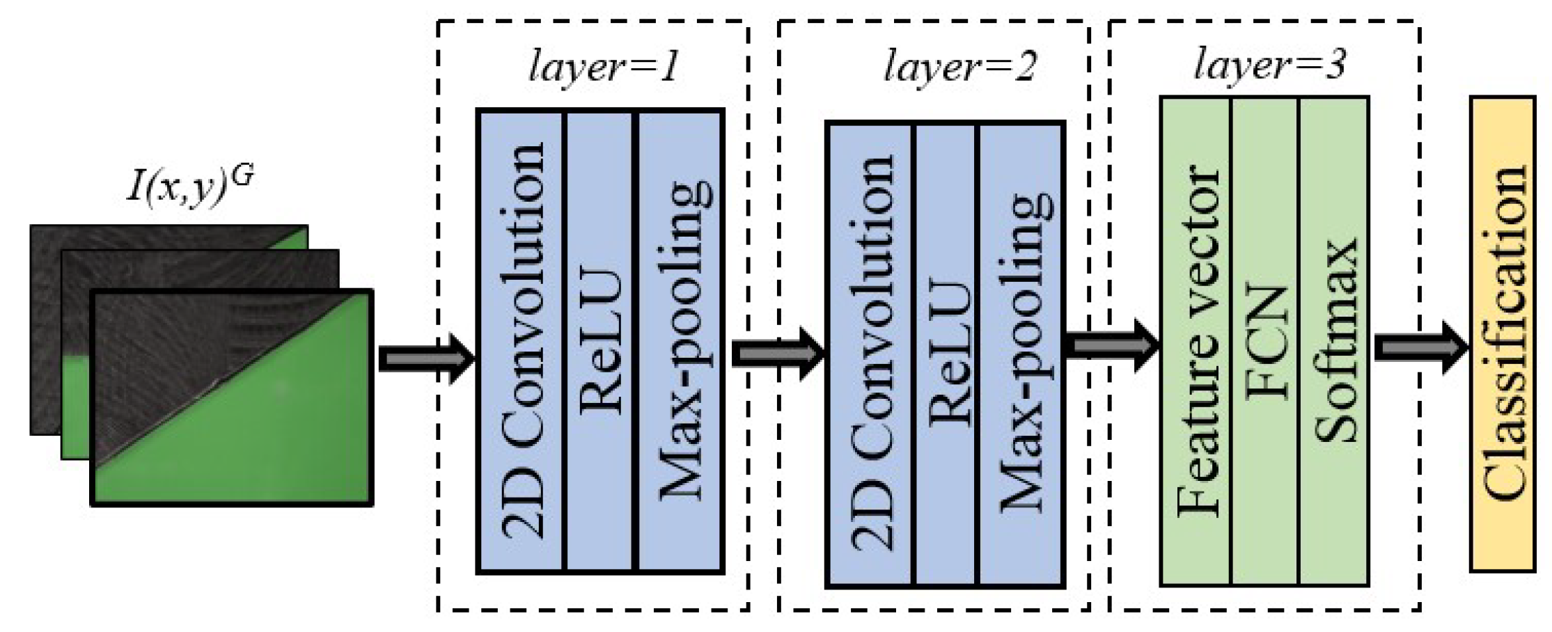
The CNN architecture comprises the input, feature extraction, and classification layers. The input is the green channel I d , β ( x , y ) G for CNNG and P d , β ( x , y ) G for CNNP. The feature extraction layer comprises two convolutional sublayers, each composed of a set of two-dimensional kernels, a ReLU activation function, and max-pooling. The first convolution sublayer has ten kernels with dimensions of ( 3 x 3 ) , and the second has 20 kernels of ( 5 x 5 ) . The result of the feature extraction layer is a vector with the abstract properties of the input.
The classification layer comprises a feature vector sublayer, a fully connected sublayer (FCN), and softmax sublayers. We used two CNNs for the experiments, shown in Figure 19, and the sublayers of the CNNs are defined in [41]. The Fourier features M Δ , β ( k ) were processed with the FFNN and the CNN with the architecture of [13]. The images I α , β ( x , y ) G and P α , β ( x , y ) were processed also with AlexNet, VGG-16, ResNet, inception presented in [14].
The networks were trained by dividing the dataset into 70% for training (250 images) and 30% for testing (106 images). The learning parameters are selected considering the networks are trained with few images. Then, the chosen optimizer is stochastic gradient descendant (SGD), the learning rate is 0.001, the batch is one, and we use 300 epochs with an early stop. According to [42], SGD performs better than SGDM, ADAM, NADAM, and RMSprop because these methods have statistical moments that reduce the oscillations during the training but reduce the generalization with few samples. The learning rate and the batch were selected to reduce the oscillations of the SGD. Also, SGD generates better performance in the experiments than SGD with momentum (SGDM), adaptive moment estimation (ADAM), Nesterov-accelerated ADAM (NADAM), and root mean square propagation (RMSprop).

4. Results

This section presents the quantitative and qualitative experiment results regarding the contour profile inspection, a machine learning analysis of classifications, a comparison of the NIIM between the CMM contact method, and a discussion.

4.1. Contour Profile Inspection

The results of the contour profile inspection are conducted by generating the signature spectrum evaluation, involving the examination of 60 signatures for each profile, encompassing four distinct materials. They are comparing the spectrum M d , β ( k ) of the calibration piece versus the spectrum M g , β ( k ) of the reference. Through the subtraction of the two spectrum signals to generate a third spectrum signal M Δ , β ( k ) that defines the profile variation.
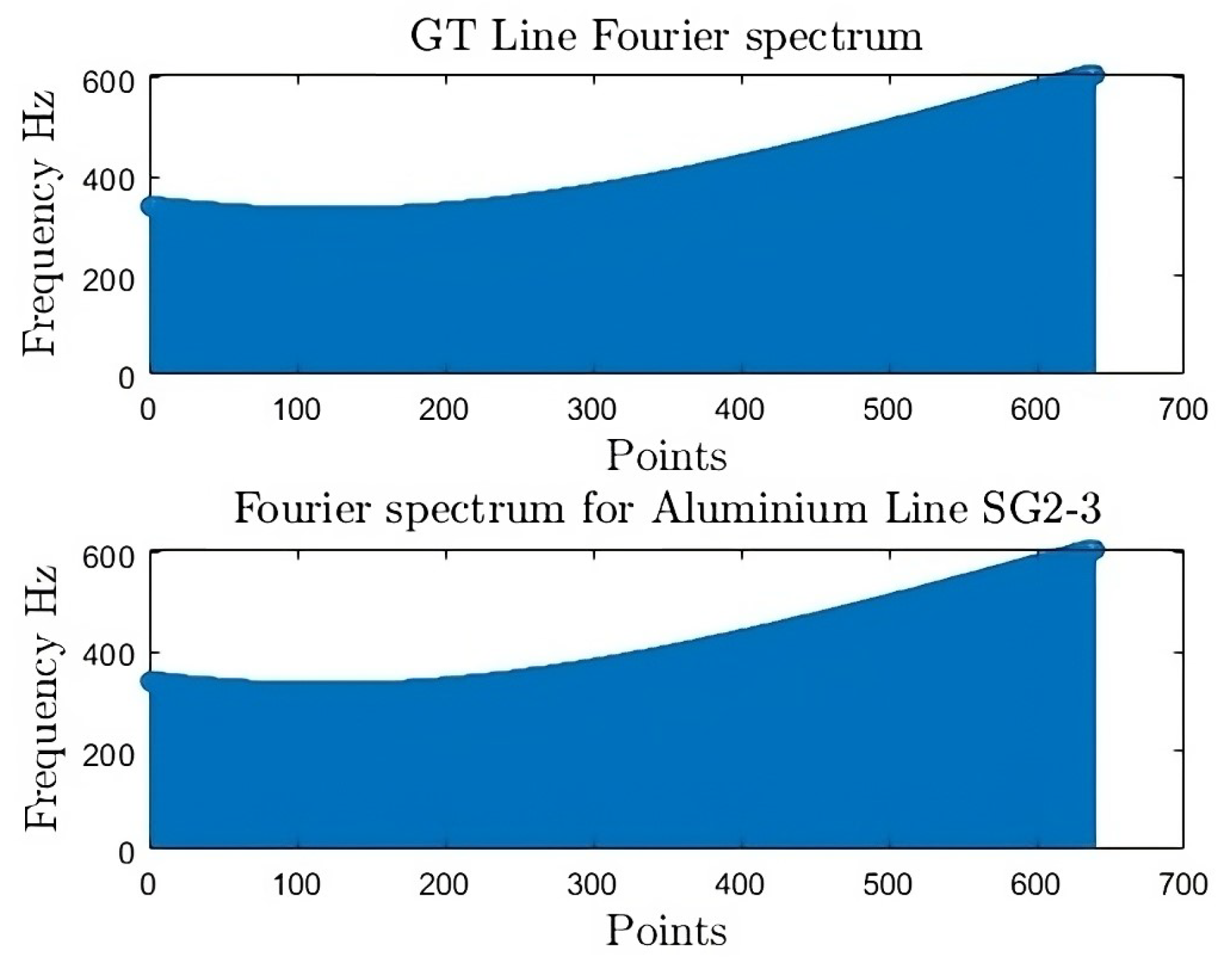
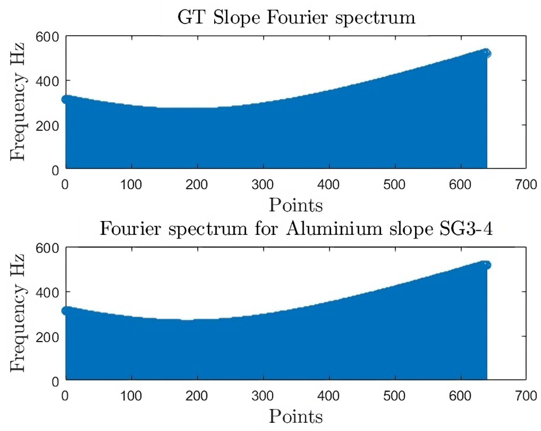
The analysis of an aluminum sample is renowned for its superior dimensional precision, making it an ideal material for evaluating profile accuracy. The examination of signature profiles I d , C ( x , y ) S G , I d , L ( x , y ) S G , and I d , S ( x , y ) S G , generate the spectrum signals M Δ , β ( k ) shown in Figure 20, Figure 21 and Figure 22.
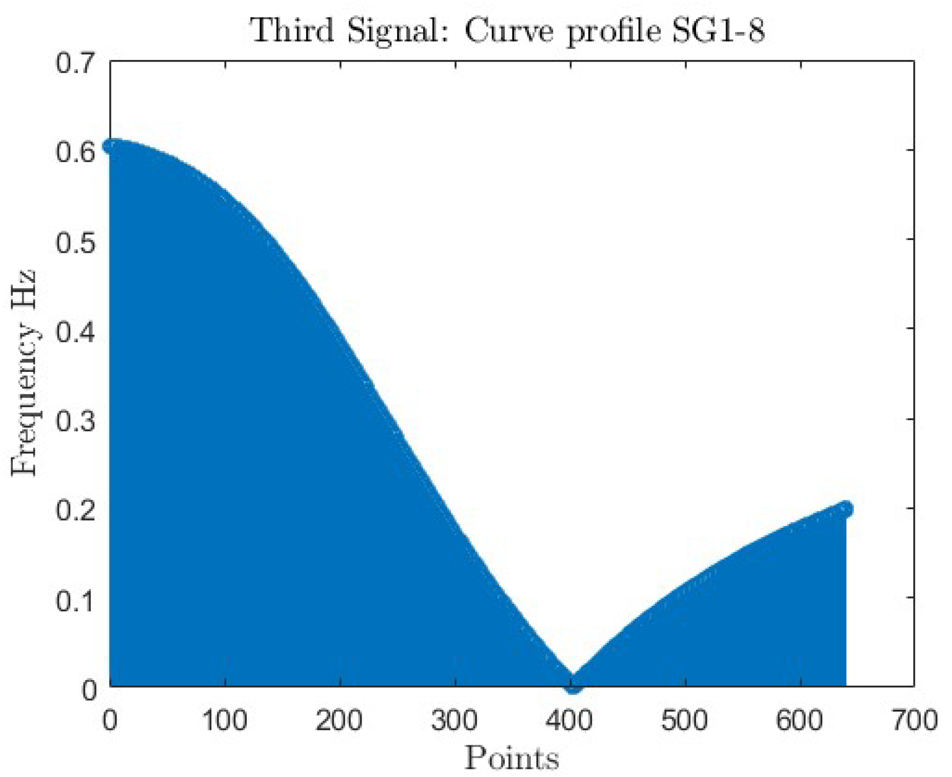
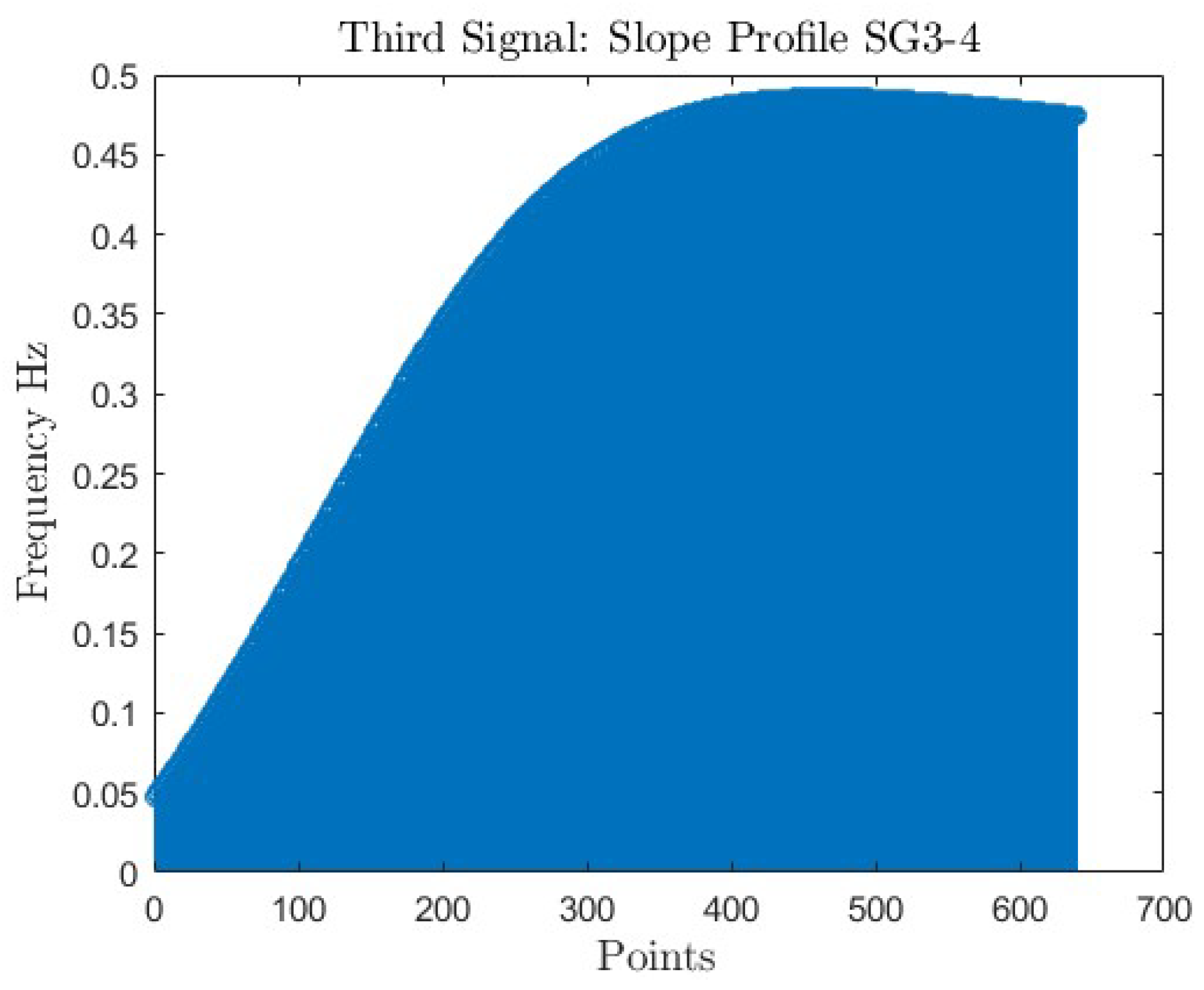
The values depicted in Figure 23, Figure 24 and Figure 25 reveal the result of the third signal spectrums for each profile signature. The maximum peaks: M Δ , C ( k ) = 0.623 for I d , C ( x , y ) S G 8 , M Δ , L ( k ) =0.556 for I d , L ( x , y ) S G 3 , and M Δ , S ( k ) =0.489 for I d , S ( x , y ) S G 4 indicates significant form deviations within each signature. However, they fall within the tolerance zone limits. The M Δ , β ( k ) numerical representations serve as a quantitative indicator, offering a precise contour profile inspection of the machined parts in each signature I d , β ( x , y ) S G . The significance of M Δ , β ( k ) values lies in the ability of the NIIM to quantitatively assess the line profile tolerance and characterize the contour profile quality, giving an impact of machining on the accuracy of each profile type, ensuring a thorough understanding of the impact of the NIIM on profile inspection accuracy.
Form deviation results are presented in a probability plot, demonstrating a systematic approach that guarantees close correspondence between the derived inspection and the genuine physical attributes of the profile. The results obtained from the analysis of each contour based on the study of its shape deviation are shown in the following subsection.

4.1.1. Form Deviation Analysis on Curve Profile

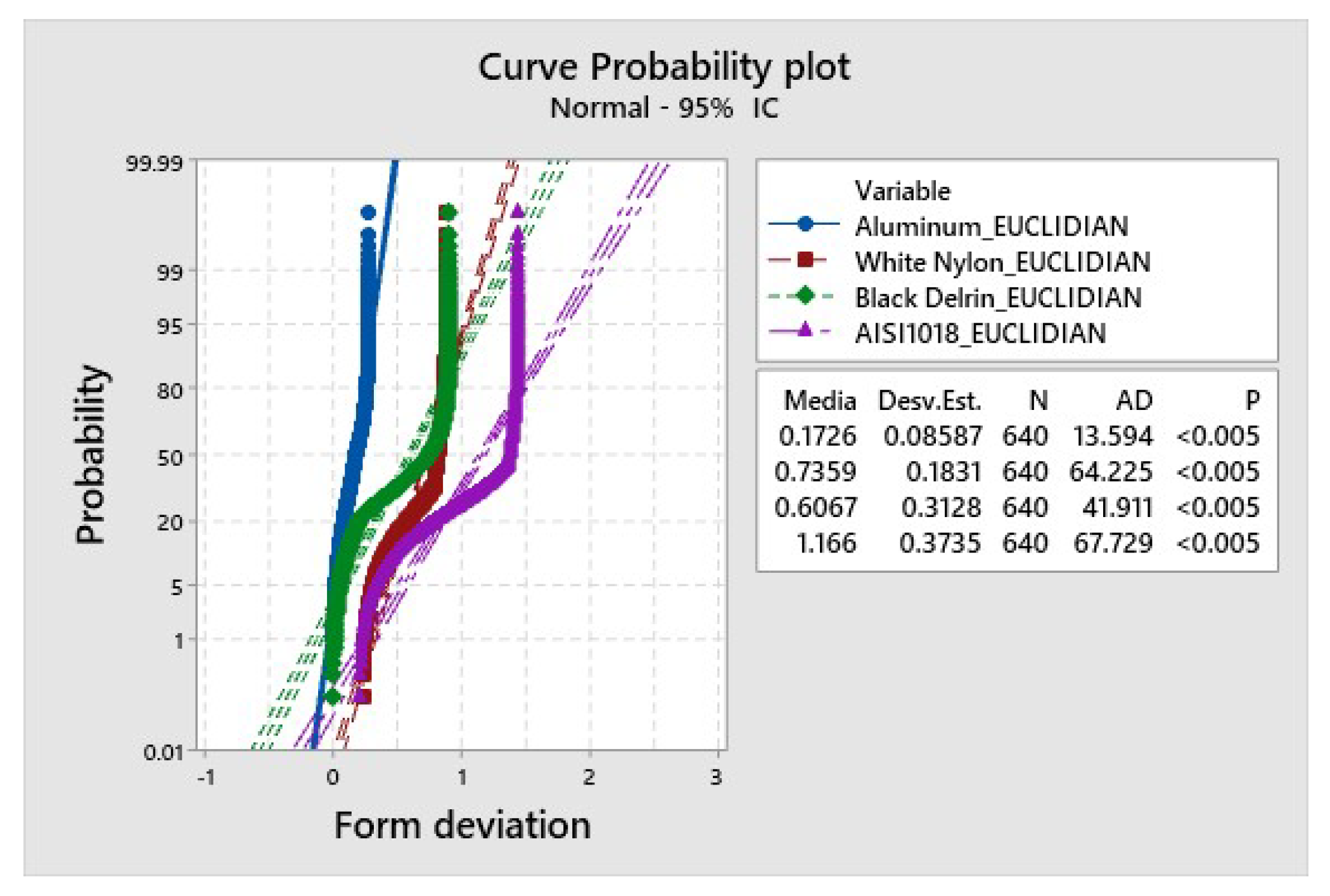
Figure 26 outlines the trends in form deviation, showing the correlation with M Δ ( k ) values obtained from the I d , C ( x , y ) S G . The materials involved in the analysis include aluminum, nylon, delrin, and steel.
It is crucial to highlight that M Δ , C ( k ) serves as an indicator for quantifying the form deviations in the curve profiles of these materials. A reduced M Δ , C ( k ) value indicates a closer adherence to the ideal curve, implying minimal form deviations. Conversely, a higher value suggests more pronounced deviations, potentially exceeding the tolerance limits.
Aluminum, with a mean of M Δ , C ( k ) =0.1726, exhibits the least form deviations among the materials under consideration. Results show that the curve profile of aluminum closely matches the ideal curve, reflecting a high degree of accuracy and precision in its manufacturing.
Nylon, with a mean M Δ , C ( k ) =0.7359, shows moderate form deviations compared to aluminum. While nylon may have some imperfections in its curve profile, the deviation is still within an acceptable tolerance, and the material can be considered suitable for certain applications.
With a mean M Δ , C ( k ) =0.6067, Delrin falls within a similar range as nylon regarding form deviations. Results imply that delrin also exhibits a moderate level of accuracy in its curve profile, making it a viable option for specific applications where such deviations are acceptable.
On the other hand, steel stands out of tolerance with a relatively higher mean M Δ , C ( k ) value of 1.16, indicating more significant form deviations than the other materials. Results may be attributed to the inherent characteristics of steel or the specific manufacturing processes involved, which result in a curve profile that deviates noticeably from the ideal.
In summary, aluminum demonstrates the least deviations, nylon and delrin exhibit moderate levels, and steel shows a higher form deviation degree.

4.1.2. Form Deviation Analysis on Line Profile

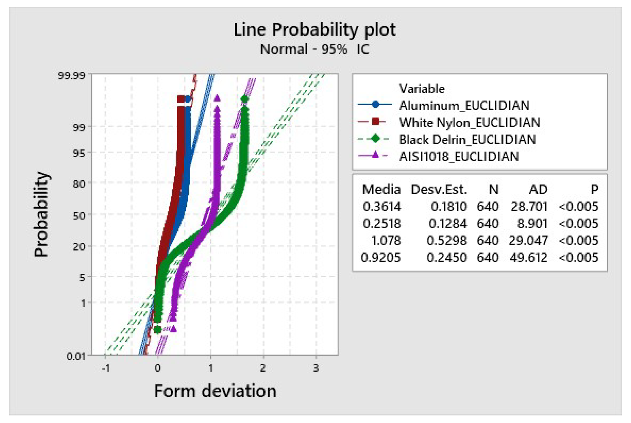
The line profile analysis presented in Figure 27 outlines the trends in form deviation, showing the correlation with M Δ ( k ) values obtained from the I d , L ( x , y ) S G . The materials involved in this analysis include aluminum, nylon, delrin, and steel.
Starting with aluminum, which has M Δ , L ( k ) = 0.3614, the analysis reveals moderate form deviations in its line profile. Results show that aluminum maintains relatively good accuracy in its line profile, but there are discernible deviations from the ideal form. This information is crucial for applications where precision in the line profile is a critical factor.
Nylon, with M Δ , L ( k ) = 0.2518, exhibits lower form deviations than aluminum. Results show that nylon’s line profile is closer to the ideal form, indicating higher accuracy and potentially making it suitable for applications where stringent form requirements are essential.
Delrin stands out with a significantly higher M Δ , L ( k ) = 1.078, signaling a more substantial level of form deviations in its line profile. This information is essential for applications where precision and conformity to the ideal form are critical, as the deviations in delrin may impact its suitability for certain use cases.
Steel, with M Δ , L ( k ) = 0.9205, demonstrates considerable form deviations in its line profile. Results show that the line profile of steel deviates noticeably from the ideal form, indicating potential challenges in applications that require high precision and accuracy.
In summary, the line profile analysis demonstrates the least deviations in nylon, the strong correlation between nylon and aluminum, and the highest form of delrin deformation. The correlation with changing machining conditions emphasizes the need for a comprehensive understanding of material properties and machining parameters to achieve the desired line profile tolerances in various applications.

4.1.3. Form Deviation Analysis on Slope Profile

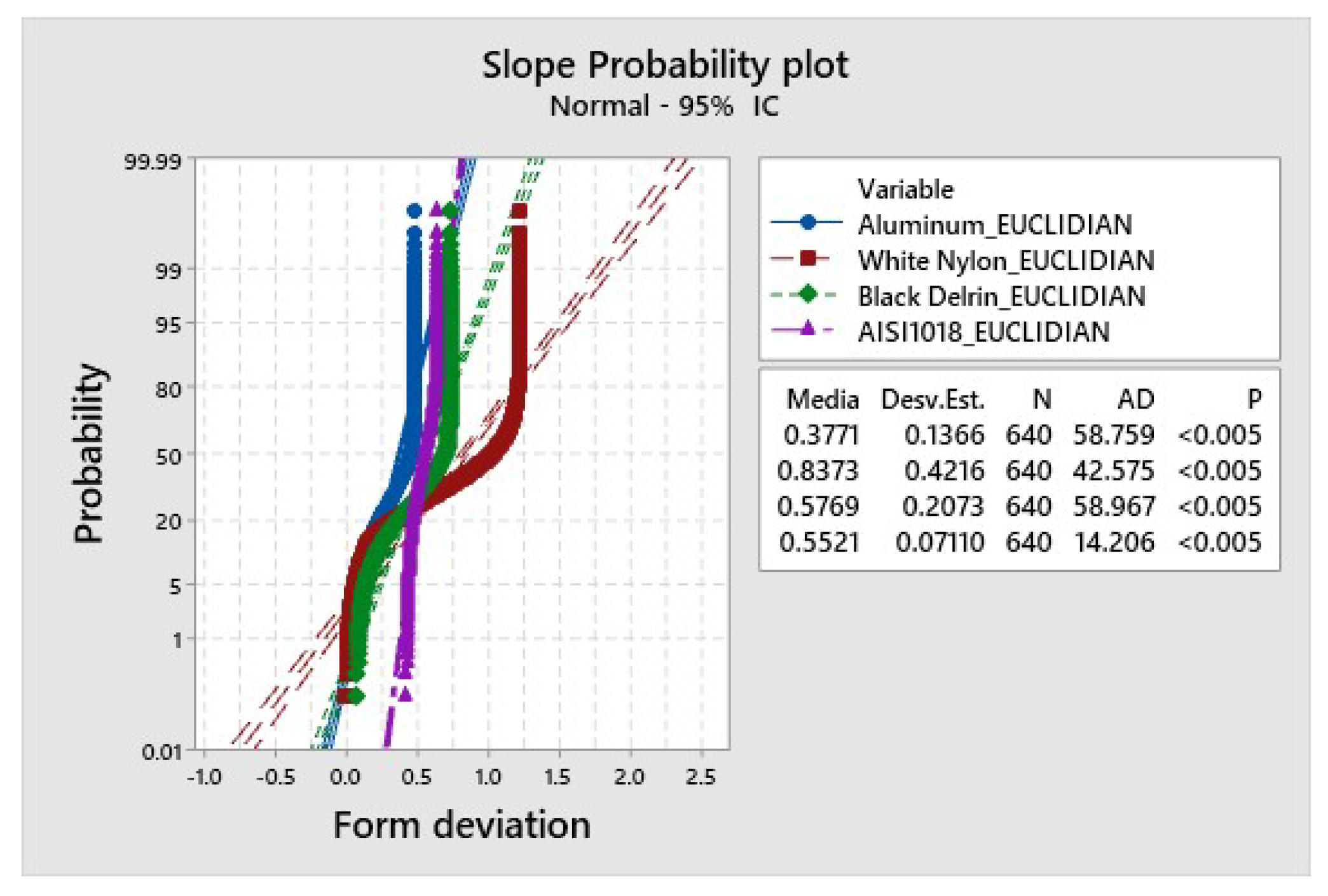
The slope profile analysis, as depicted in Figure 28 outlines the trends in form deviation, showing the correlation with M Δ ( k ) values obtained from the I d , S ( x , y ) S G . The materials involved in this analysis include aluminum, nylon, delrin, and steel.
Beginning with aluminum, which has M Δ , S ( k ) = 0.3771, the slope profile analysis reveals moderate form deviations. Results show that the slope profile of aluminum exhibits noticeable variations from the ideal form, emphasizing the importance of understanding these deviations in applications where slope precision is critical.
Nylon, with M Δ , S ( k ) = 0.8373, exhibits higher form deviations in its slope profile than aluminum. Results indicate that nylon is out of tolerance for essential applications where slope accuracy is paramount. The nylon deviations may impact suitability for certain use cases requiring precise slope control.
With M Δ , S ( k ) = 0.5769, Delrin presents a moderate range of form deviations in its slope profile. Understanding these deviations is crucial for applications that demand a specific slope precision, as delrin may display variations that must be considered in the design and manufacturing processes.
Steel, with M Δ , S ( k ) = 0.5521, demonstrates a relatively low level of form deviations in its slope profile. Results show that the slope profile of Steel is closer to the ideal form, making it potentially well-suited for applications requiring precise slope control.
Similar to the previous analyses, the correlation between varying machining conditions and distinct levels of profile form deviations is highlighted in the slope profile analysis. Results demonstrate correlation and underscore the importance of considering the influence of machining parameters, such as cutting speeds, feeds, and tool geometries, on the slope precision of these materials. Adjustments in machining conditions may be explored in future research to minimize slope deviations and enhance the overall accuracy of slope profiles.

4.2. Machine Learning Results

The machine learning models rFFNN, mFFNN, kFFNN, CNNG, CNNP, SVM, LSTM, AlexNet, ResNet, VGG-16, and Inception were evaluated to determine which feature vector and network are the best option for shape and quality contour profile classification.
According to [3,4,6,15,16] y [38], the metrics used to know the performance is accuracy for training and test (TAcc and PAcc, respectively), and Confusion matrices, defined in [13,14]. Also, we include computational cost metrics such as frame per second (FPS) and the number of parameters (NPam) to know which network is feasible for real-time processing in industrial environments for inspection applications.
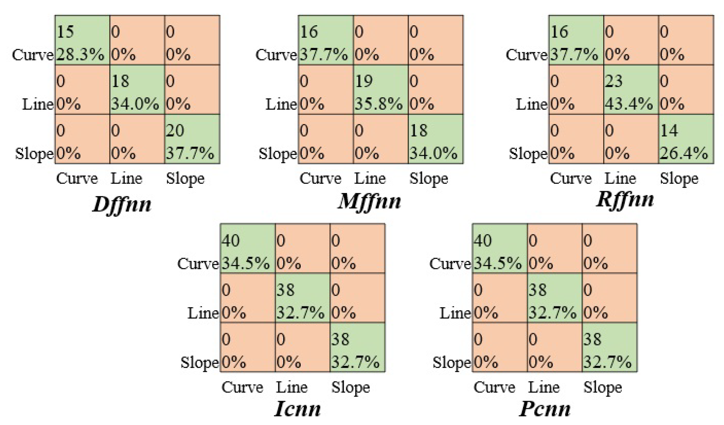
Contour profile Classification. The NIIM classifies contour calibration pieces into Curve, Line, and Slope categories in terms of quality. The feature vector r d , β ( n ) has a size of 508 elements. In contrast, the feature vectors M d , β ( k ) and D Δ , β ( k ) have a size of 150 because, according to our experiments, the frequencies 0 < k < 100 are enough to represent the shape in the frequency domain. The networks rFFNN, mFFNN, and kFFNN have six neurons in the hidden layers and were tested with five validation experiments. Table 6 shows the results where the networks rFFNN, mFFNN, kFFNN, CNNG, and CNNP achieved 100% for training and testing. However, mFFNN and kFFNN are faster and have fewer parameters than the others.
Figure 29 presents the confusion matrices of rFFNN, mFFNN, kFFNN, CNNG, and CNNP, where the performance is the same. However, kFFNN presents less overfitting during the training. Regarding converging epochs, rFFNN requires 56 epochs, mFFNN 28, kFFNN 25, CNNG 15, and CNNP 10. CNNG and CNNP require fewer epochs to converge than the other networks, but they present more overfitting than kFFNN. SVM, LSTM, AlexNet, VGG-16, ResNet, and Inception networks require 300 epochs.
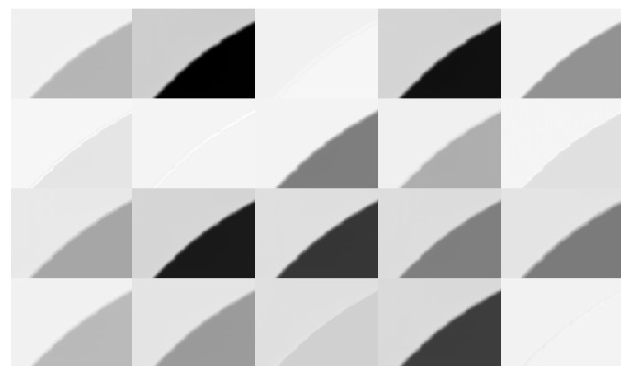
CNNG learns features based on the piece surface and the illumination of the vision system, while CNNP learns features of the profile shape. For example, Figure 30 shows the second convolution activation maps, where the propagation of a curve image generates activation divided into the piece surface and the illumination.
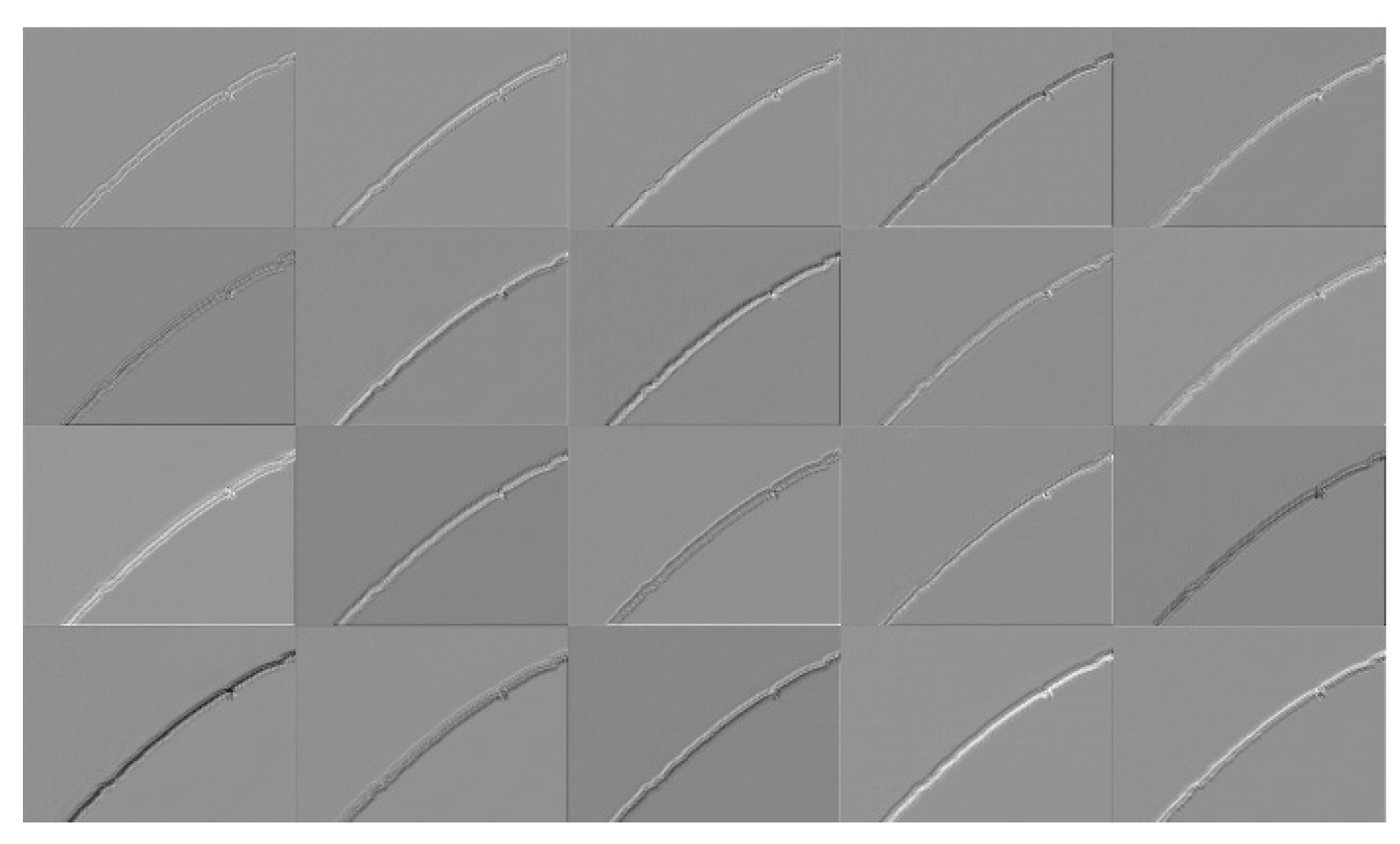
Figure 31 shows the activation maps of the second convolution layer, where the propagation of a curve image generates activation with similar patterns to the Laplacian filtering.
rFFNN, mFFNN, CNNG, and CNNP achieve good results because they learn the shape features that have r d , β ( n ) , M d , β ( k ) , I d , β ( x , y ) G , and P d , β ( x , y ) . Additionally, kFFNN generates good results because D Δ , β ( k ) have form deviation properties derived from the three machined processes that generate Curve, Line, and Slope profiles. Added to this, kFFNN and mFFNN generate the lowest computational cost. The models SVM, LSTM, AlexNet, VGG-16, ResNet, and Inception generate less accuracy than the FFNNs and CNNs proposed in this work. SVM has three lineal discriminant functions, each with 251 parameters (one for each feature vector and the bias).
However, the low accuracy is due to the shape classes being overlapped in the frequency feature space. The LSTM has low accuracy because it interprets a false causal relation between frequencies. The CNNs AlexNet, VGG-16, ResNet, and Inception have many parameters that codify many feature maps during propagation with irrelevant information and properties for shape classification.
Quality classification. The NIIM classifies calibration pieces into normal and defect-calibration pieces. For task classification, the feature vector r d , β ( n ) has a size of 508 and the feature vectors M d , β ( k ) and D Δ , β ( k ) have a size of 168 because, according to our experiments, the frequencies 2 < k < 170 are enough to represent the quality of the contour profile in the frequency domain.
The contour profile signature was selected because, according to [40], profile quality defects and form deviations affect wear resistance, tolerance accuracy, shape deformation, fatigue resistance, corrosion resistance, and fluid passage in the milling part.
An expert generates the ground truths for task classification by dividing the dataset considering the geometric dimension and tolerances according to ASME Y14.5.1M and ISO/TC 213 for machine learning purposes.
Concerning the metrics of the experiments and results, we add the F-measure (F1) metric because it is used in many works as used in [13,14] and is defined as the harmonic mean between precision and recall in binary classifications.
The NIIM considers the true positive when a normal piece is classified as normal. The networks rFFNN, mFFNN, and kFFNN have 48 neurons in the hidden layers, and they were tested with five validation experiments. Regarding converging epochs, rFFNN requires 69, mFFNN 100, kFFNN 110, CNNG 32, and CNNP 32. CNNG and CNNP require fewer epochs to converge than the other networks, but after 32 epochs, they cannot improve the accuracy. SVM, LSTM, AlexNet, VGG-16, ResNet, and Inception networks require 300 epochs.
Table 7 shows the results of the experiments in quality classification, where kFFNN presents the best performance and computational cost because D Δ , β ( k ) describes the form deviation generated by the machined process. rFFNN and mFFNN had low performance in the test and training because the input feature vectors of r α , β ( n ) and M d , β ( k ) concentrate most of their energy on shape features. Hence, these vectors feed the ANN with few form deviation features. The CNN networks had good accuracy during the training, but the accuracy during the test decreased significantly. This performance is because of overfitting generated by many features unrelated to the contour profile.
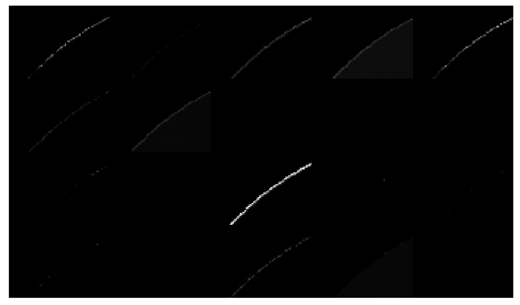
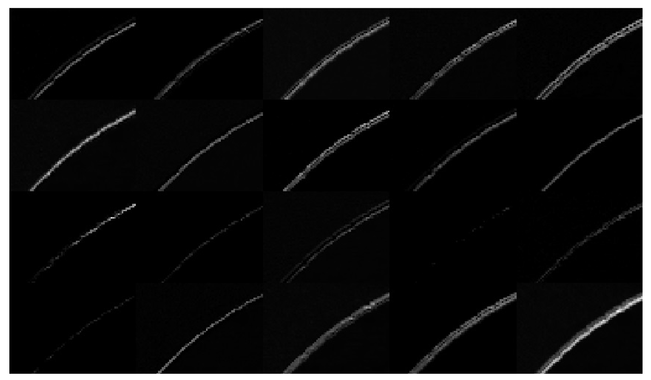
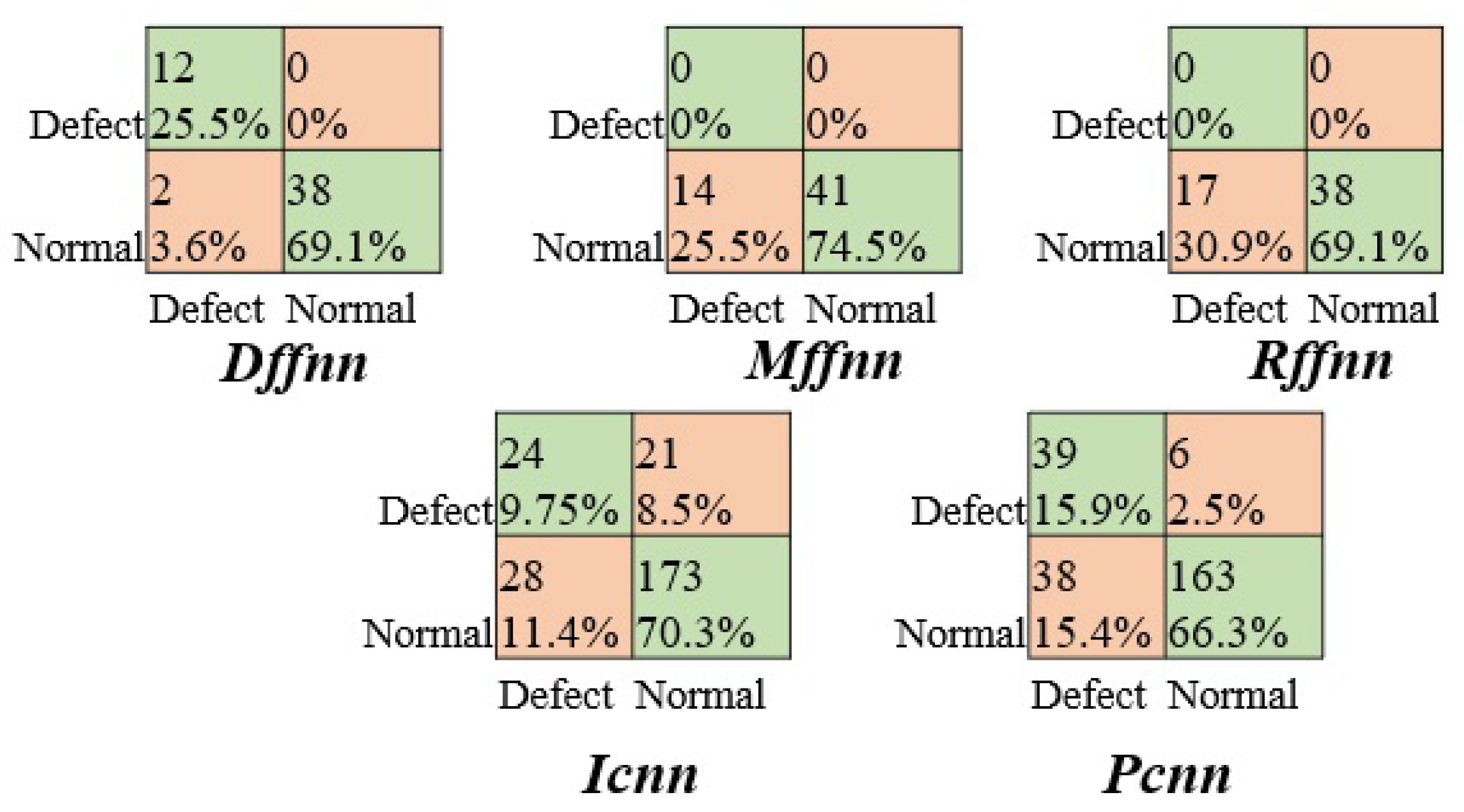
Figure 32 and Figure 33 show the second layer activation maps of CNNG and CNNP trained considering the normal and defective classes, where the features learned are focused on the shape properties. Then, rFFNN, mFFNN, CNNG, and CNNP process shape rather than form deviation features because the energy of the features is mainly concentrated in shape features. kFFNN achieves good results and has the lowest computational cost because it has only deviation features that describe the milling process in the piece. Figure 34 shows the contour profile classification confusion matrices. mFFNN and rFFNN classified all samples as normal, and CNNG and CNNP classified half of the defective samples as normal.
SVM, LSTM, AlexNet, VGG-16, ResNet, and Inception models generate less accuracy and F1 than the FFNN and CNNs proposed in the NIIM. SVM has low accuracy because the shape classes overlap in the frequency feature space. The LSTM has low accuracy because it interprets a false causal relation between frequencies. The CNNs AlexNet, VGG-16, ResNet, and Inception are networks with many parameters that codify many feature maps during propagation with irrelevant information and properties for quality classification.

4.2.1. Computational Cost

Table 6 and Table 8 show that kFFNN and mFFNN achieve the best FPS and Number of variables, and Table 9 presents the relation of NPam of CNNG, CNNP, and rFFNN against NPam of kFFNN and mFFNN. The differences in the computational costs are because I α , β ( x , y ) G and P α , β ( x , y ) have 307,200 elements and many abstract features that the CNNs need to codify. The rFFNN processes the signals r α , β ( n ) , which have 600 to 640 elements and are time-domain signals with shape, form deviation, and resolution error features. On the other hand, M Δ , β ( k ) and D Δ , β ( k ) have 150 or 170 elements that represent the shape and form deviation features.
The computational performance of renowned networks such as AlexNet [45], VGG-16, ResNet [46], comes at a higher cost, resulting in accuracy levels below 85% for shape and quality classification. The results are attributed to the networks’ tendency to learn redundant features, which may not contribute significantly to the classification task. Moreover, their computational demands render them impractical for real-time processing, as the frames per second (FPS) achieved are not conducive to swift and efficient analysis.
According to the machine learning experiments, any ANN with r α , β ( n ) , M α , β ( k ) , or I α , β ( x , y ) G and P α , β ( x , y ) generate good performance in shape classification, but regular results in quality classification. The results are obtained because these inputs concentrate the energy in shape information and have little energy in form deviation information. Then, the ANN cannot learn from the form deviation features.
On the other hand, D Δ , β ( k ) and the FFNN generate the best computational cost and good performance in shape and quality classification. These results are obtained because D Δ , β ( k ) have only deviation features, and the tolerance zone is represented with 100 frequency elements (it can be seen in Section 2.3.3. The obtained performance of D Δ , β ( k ) is because the form deviation feature vector is a signature of the CNC milling process that generates the profile of the calibration piece.
Also, according to the discussion section, the D Δ , β ( k ) feature vector generates high energy when the piece has a shape deformation and can be used to identify if the profile machine process accomplishes the geometric standard tolerances.
5. Discussion

The energy of the calibration piece form deviation refers to the distribution of microscopic peaks and valleys not defined in the GT profiles. A metric known as the energy of D Δ , β ( k ) is implemented to quantify and analyze these characteristics. The D Δ , β ( k ) metric represents the displacement of the milling part, peaks, and residue of the machining process defined as:
E = 1 N k = 0 N 1 D Δ , β ( k ) 2
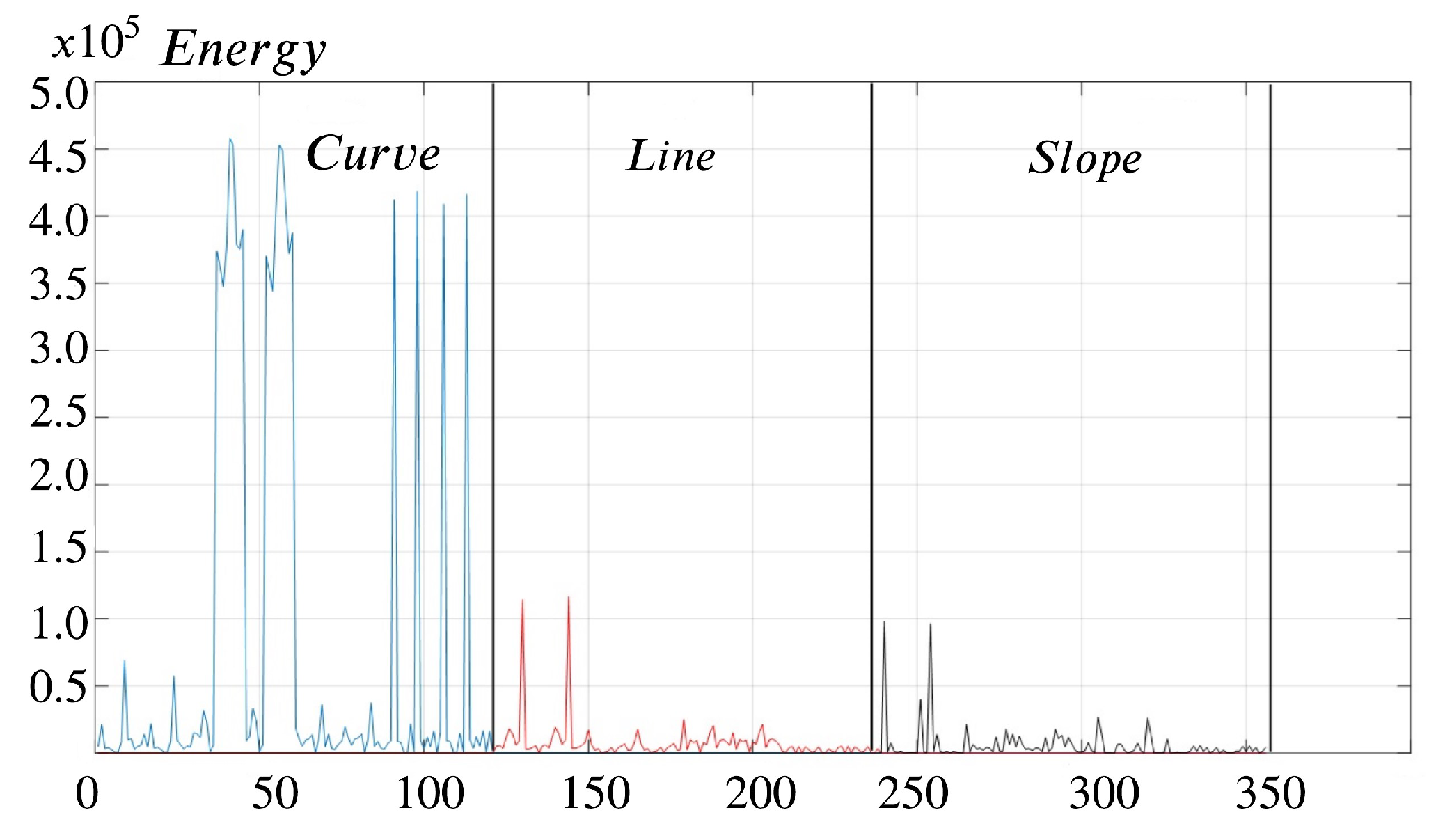
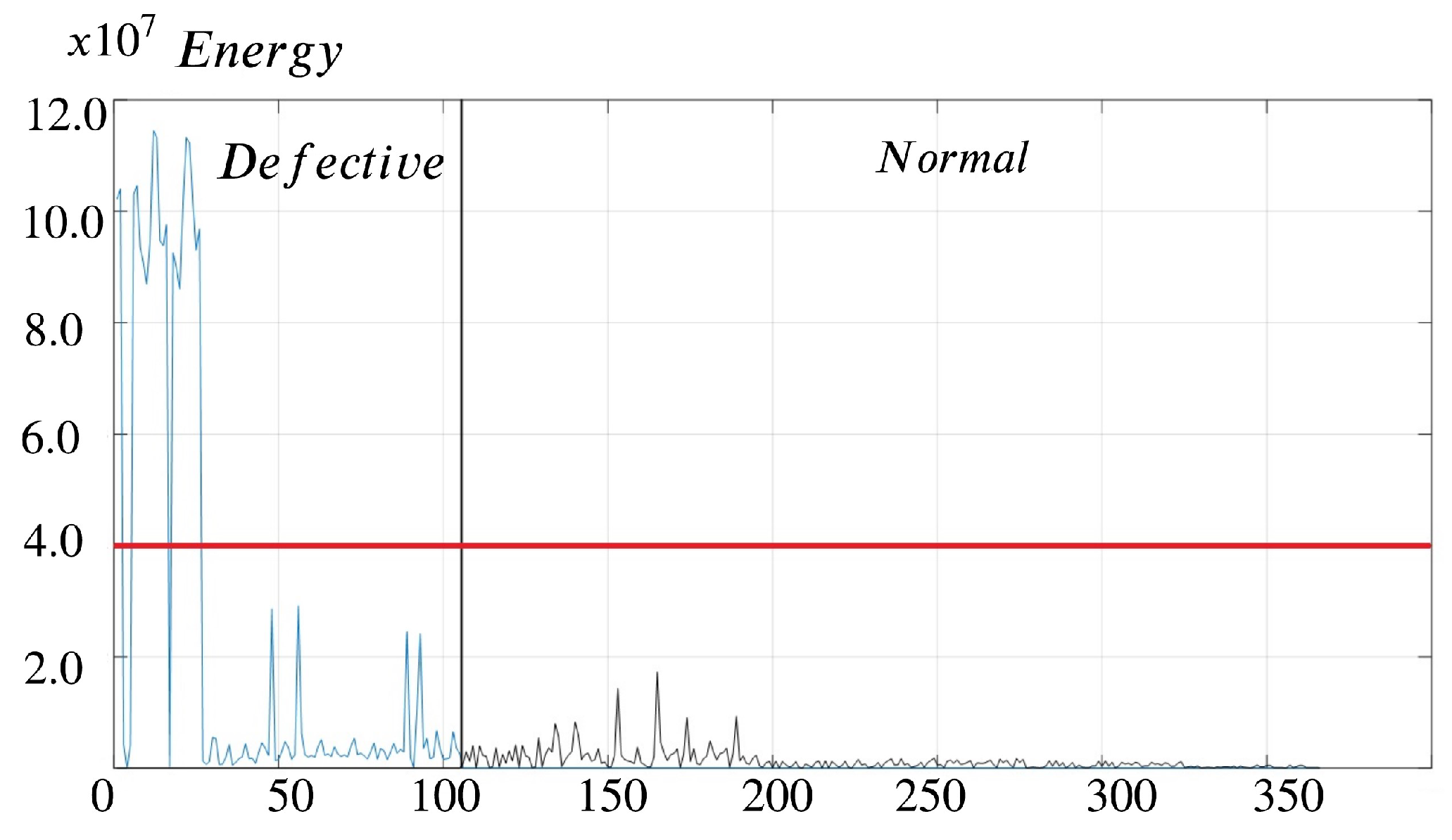
The results of the energy analysis for the calibration pieces are illustrated by shape in Figure 35 and by quality in Figure 36. Based on D Δ , β ( k ) analysis, it becomes evident that the curve generates more energy compared to the line and slope. The heightened energy output can be attributed to the inherent complexities of machining curves, especially in scenarios where the machine simultaneously interpolates the X and Y axes to conform to the specified radius.
When machining a curve, the machinery coordinates the movement along two axes simultaneously, necessitating a more intricate interpolation process. The dual-axis interpolation demands the machine’s capabilities, requiring it to precisely synchronize movements to conform to the curvature specified in the program. The intricate nature of this simultaneous interpolation results in increased energy consumption during the machining process, as compared to simpler geometries like a straight line or a slope. Regarding contour profile quality, calibration pieces with form deviation defects generate more energy during machining due to the inherent challenges of irregular surface features.
The energy generated in the slope, line, and curve profiles varied for delrin, nylon, aluminum, and steel. delrin exhibits low energy generation, nylon exhibits high energy generation, and aluminum exhibits moderate energy generation. These differences are primarily influenced by the friction coefficients of the materials and their resistance to deformation under stress [47].
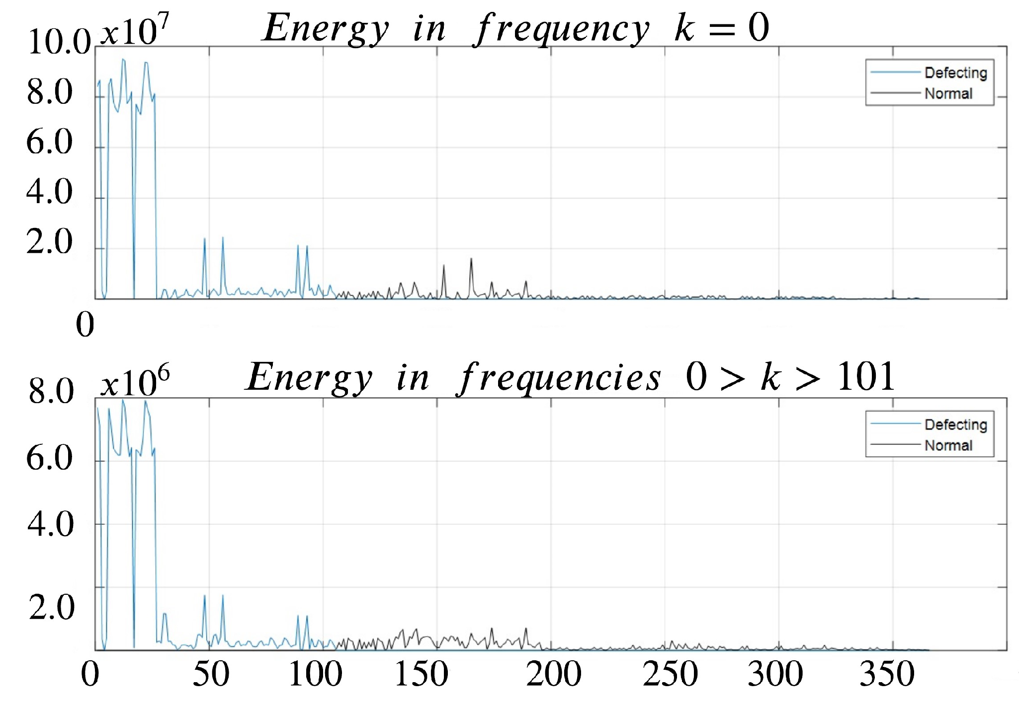
Figure 37 displays the energy at zero frequency and the frequencies 0 < k > 101 of D Δ , β ( k ) . The amplitude at zero frequency corresponds to millimetric displacements between the calibration piece placement in the Fixture and the zero position. Within the bandwidth 1 < k < 100 for all samples, the energy is non-zero, indicating that small-scale variations in height actively contribute to the texture or deviations of the profile. Remarkably, the curve defective pieces exhibit notably higher energy levels at zero and low frequencies. This heightened energy is attributed to the specific challenges associated with machining irregularities on the curved surface.

5.1. Comparison Between CMM and NIIM

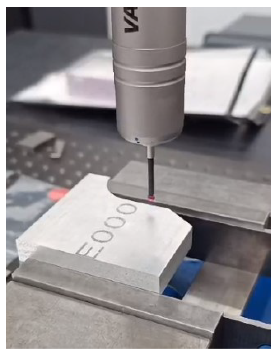
A comparative analysis between NIIM and contact measurement was performed using a coordinate measuring machine (CMM) to assess the reliability of the proposed method. The calibration pieces used for the study were aluminum and were mounted in the CMM surface plate referenced to datums A and B as shown in Figure 38.
The measuring of the profile of a line tolerance by CMM was performed based on the direction vector method [48], involving the assessment of 152 points from point C to D for each cross-section. Direction vectors were defined to direct the probe along the contour profile, enabling the capture of data points at predetermined positions. A 2 mm ball diameter probe was utilized to record multiple measurements and juxtapose them with a virtual boundary to measure the profile line.
Figure 39 illustrates the average deviation results of the profile of the line measures obtained by CMM. The upper label, 75.19549, corresponds to the overall profile of a line, while the lower label, 74.91963, pertains to the per-unit profile of a line. Notably, in both instances, the average 0.71579 deviation falls within the prescribed tolerance zone limits.
Subsequently, a measurement study was conducted on the repeatability, reproducibility, and total Gage R&R for the 152 discrete points evaluating the average deviation, using ten calibration pieces with three operators in three series. The results of these analyses are presented in Table 10 and Table 11. Specifically, the 95th percentile values for σ R & R were determined to be 7.9% for the NIIM and 10.9% for the CMM.
The data in Table 10 show that the CMM R&R study presents a lower form deviation measurement than the NIIM R&R Study. However, the practical importance of this difference is relatively small and falls within acceptable industry standards. CMM and NIIM satisfy the criteria of an R&R study according to common benchmarks, which aim for a Gage R&R tolerance of under 30%. However, the advantage of the NIIM lies in its significantly faster inspection time and lower computational costs. These factors essentially determine the reliability of the NIIM system.
Finally, to evaluate the effectiveness of NIIM, an error study was computed to measure the contour profile form deviations obtained from CMM and NIIM. This assessment, as described in [49], involves the average relative error (ARE), the root mean square error (RMSE), and the correlation coefficient R 2 represented by Equations 8, 9, and 10 respectively. The resulting metrics are summarized in Table 12.
A R E = 1 n i = 1 n y i y ^ i y i
R M S E = 1 n i = 1 n ( y i y ^ i ) 2
R 2 = 1 i = 1 n ( y i y ^ i ) 2 i = 1 n ( y i y ¯ ) 2
where n is the number of the form deviation observations, y i are the actual form deviation values, and y ^ i are the predicted form deviation values.
In the results between CMM and NIIM, several observations can be made: CMM demonstrates a lower ARE (0.0257) than NIIM (0.0301), indicating slightly better performance regarding the average error. Similarly, CMM exhibits a lower RMSE (0.0781) than NIIM (0.0812), suggesting slightly better overall accuracy in measurements. CMM shows a higher R 2 (0.9318) than NIIM (0.9265), implying a stronger linear relationship between predicted and observed values for CMM measurements. CMM achieves a slightly higher accuracy of 97.43% compared to NIIM’s accuracy of 96.99%.

6. Conclusions

According to the machine learning experiments, D Δ , β ( k ) and the FFNN generate the best computational cost and good performance in shape and quality classification. The results are obtained because D Δ , β ( k ) have only deviation features, and the tolerance zone is represented with 100 frequency elements (it can be seen in Section 2.3.3. The obtained performance of D Δ , β ( k ) is because the form deviation feature vector is a signature of the CNC milling process that generates the profile of the calibration piece. Also, according to the discussion section, the D Δ , β ( k ) feature vector generates high energy when the piece has a shape deformation and can be used to identify if the profile machine process accomplishes the geometric standard tolerances. CNNs with r α , β ( n ) , M α , β ( k ) , or I α , β ( x , y ) G and P α , β ( x , y ) generate good performance in shape classification, but regular results in quality classification.
The results are obtained because the inputs concentrate the energy in shape information and have little energy in form deviation information. Then, the CNNs generate features unrelated to deviation and quality contour shape profiles. SVM and SLTM methods generate regular results in shape and quality classification due to overlap between classes and misinterpretation of contour frequencies. The networks VGG-16, ResNet, and Inception generate regular results because they analyze many abstract features irrelevant to shape and quality analysis.
In summary, while contact measurement methods like CMM offer marginally better accuracy in certain metrics, NIIM offers 96.99% accuracy, low computational requirements, 100% inspection capability, quality classification, and overall effectiveness positioning. NIIM is a compelling alternative for organizations seeking efficient and reliable inspection solutions.

Author Contributions

M. Meraz and J. Ramírez proposed the methodology and prepared the original draft; M. Nandayapa and O. Vergara validated the obtained results; E. Reynoso edited the final paper. All authors have read and agreed to the published version of the manuscript.

Institutional Review Board Statement

Not applicable

Informed Consent Statement

Not applicable

Data Availability Statement

The raw data supporting the conclusions of this article will be made available by the authors upon request

Acknowledgments

The authors express their gratitude for the support received in various areas from the TecNM - Instituto Tecnológico de Chihuahua (Digital Signal Processing and Artificial Intelligence Lab), the Universidad Autónoma de Ciudad Juárez (Department of Industrial and Manufacturing Engineering), the Universidad Tecnológica de Chihuahua (Department of Industrial Maintenance Engineering) and Ing. Raul Villareal for scientific collaboration and the ease of use of equipment and laboratories

Conflicts of Interest

The authors declare no conflicts of interest.

References

  1. Bolar, Gururaj and Das, Argha and Joshi, Shrikrishna N."Measurement and analysis of cutting force and product surface quality during end-milling of thin-wall components" Measurement, Elsevier, vol 121, pp 190–204, 2018.
  2. Jia, Zhen-yuan and Ma, Jian-wei and Song, De-ning and Wang, Fu-ji and Liu, Wei, "A review of contouring-error reduction method in multi-axis CNC machining" International Journal of Machine Tools and Manufacture, vol 125, pp 34–54, 2018, Elsevier.
  3. Zhou, Yang and Liu, Changfu and Yu, Xinli and Liu, Bo and Quan, Yu, "Tool wear mechanism, monitoring and remaining useful life (RUL) technology based on big data: a review", SN Applied Sciences, vol 4, no. 8, page 232, 2022, Springer.
  4. , Shen, Yan and Yang, Feng and Habibullah, Mohamed Salahuddin and Ahmed, Jhinaoui and Das, Ankit Kumar and Zhou, Yu and Ho, Choon Lim, "Predicting tool wear size across multi-cutting conditions using advanced machine learning techniques" Journal of Intelligent Manufacturing, vol 32, pp 1753–1766, 2021, Springer.
  5. Duan, Zhenjing and Li, Changhe and Zhang, Yanbin and Yang, Min and Gao, Teng and Liu, Xin and Li, Runze and Said, Zafar and Debnath, Sujan and Sharma, Shubham, "Mechanical behavior and Semiempirical force model of aerospace aluminum alloy milling using nano biological lubricant", Frontiers of Mechanical Engineering,vol. 18, no. 1, pp.4, 2023, Springer. [CrossRef]
  6. , Navarro-Devia, John Henry and Chen, Yun and Dao, Dzung Viet and Li, Huaizhong, "Chatter detection in milling processes—a review on signal processing and condition classification", The International Journal of Advanced Manufacturing Technology, vol 125, no 9, pp 3943–3980, 2023, Springer.
  7. Tan-Quang Duong, Pedro Rodriguez-Ayerbe, Sylvain Lavernhe, Christophe Tournier and Didier Dumur, “Contour error pre-compensation for five-axis high speed machining: offline gain adjustment approach,” The International Journal of Advanced Manufacturing Technology, vol. 100, pp. 3113–3125, 2019. [CrossRef]
  8. Liu, Dewei and Li, Changhe and Dong, Lan and Qin, Aiguo and Zhang, Yanbin and Yang, Min and Gao, Teng and Wang, Xiaoming and Liu, Mingzheng and Cui, Xin and others, "Kinematics and improved surface roughness model in milling" The International Journal of Advanced Manufacturing Technology, vol 131, no 5, pp 2087–2108, 2024, Springer.
  9. N.K. Myshkin, A.Ya Grigoriev, S.A. Chizhik, K.Y. Choi and M.I. Petrokovets, “Surface roughness and texture analysis in microscale,” Wear, vol. 254, no 10, pp. 1001–1009, Jul 2003. [CrossRef]
  10. Chi-Fai Cheung and Wing Bun Lee, “A multi-spectrum analysis of surface roughness formation in ultra-precision machining,” Precision Engineering, vol. 24, no 1, pp. 77–87, Jan 2000. [CrossRef]
  11. DVN Prabhakar, M Sreenivasa Kumar and A Gopala Krishna, “A Novel Hybrid Transform approach with integration of Fast Fourier, Discrete Wavelet and Discrete Shearlet Transforms for prediction of surface roughness on machined surfaces. Measurement, 2020; 164, 108011.
  12. Kochetkov, AV and Troshin, AA and Zakharchenko, M Yu and Zakharov, OV, “Selection of Filter Methods in the Analysis and Measured of Geometry and Surface Roughness,” 2020 International Multi-Conference on Industrial Engineering and Modern Technologies (FarEastCon), IEEE.
  13. Ross, Nimel Sworna and Shibi, C Sherin and Mustafa, Sithara Mohamed and Gupta, Munish Kumar and Korkmaz, Mehmet Erdi and Sharma, Vishal S and Li, "Measuring Surface Characteristics in Sustainable Machining of Titanium Alloys Using Deep Learning-Based Image Processing". IEEE Sensors Journal 2023, 23, 13629–13639.
  14. Ross, Nimel Sworna and Sheeba, Paul T and Shibi, C Sherin and Gupta, Munish Kumar and Korkmaz, Mehmet Erdi and Sharma, Vishal S, "A novel approach of tool condition monitoring in sustainable machining of Ni alloy with transfer learning models", Journal of Intelligent Manufacturing, vol 35, no 2, pp 757–775, 2024, Springer. [CrossRef]
  15. Myrsini Ntemi, Spyridon Paraschos, Anastasios Karakostas, Ilias Gialampoukidis, Stefanos Vrochidis, and Ioannis Kompatsiaris. “Infrastructure monitoring and quality diagnosis in CNC machining: A review. CIRP Journal of Manufacturing Science and Technology 2022, 38, 631–649.
  16. Mohsen Soori, Behrooz Arezoo, Roza Dastres. “Machine learning and artificial intelligence in CNC machine tools, A review,” Sustainable Manufacturing and Service Economics, 2023.
  17. J Ali, H Jailani and M Murugan, “Surface roughness evaluation of electrical discharge machined surfaces using wavelet transform of speckle line images,” Measurement, vol. 149, pp. 107029, Jan 2020. [CrossRef]
  18. Joshi Ketaki and Patil Bhushan, “Evaluation of surface roughness by machine vision using neural networks approach,” in Recent Advances in Mechanical Infrastructure, Singapore, Springer, 2019.
  19. Nouhi Sepehr and Pour Masoud, “Prediction of surface roughness of various machining processes by a hybrid algorithm including time series analysis, wavelet transform and multi-view embedding,” Measurement, vol. 184, pp. 109904, Nov 2021. [CrossRef]
  20. Tushar Jain,“Industrial objects recognition in intelligent manufacturing for computer vision,” International Journal of Intelligent Unmanned Systems, vol. 10, no. 4, pp. 401–415, Nov 2021.
  21. SD Pande and MS Rani Chetty, “Position invariant spline curve based image retrieval using control points,” Int Journal Intell Eng Syst, vol. 12, no. 4, pp. 177–191, Aug 2019. [CrossRef]
  22. Tesfahun Tigistu and Getachew Abebe,“Classification of rose flowers based on Fourier descriptors and color moments. Multimedia Tools and Applications 2021, 80, 36143–36157. [CrossRef]
  23. Ahammad Hossain, Md Sojib Kaisar and Md Abdul Hakim Khan, “A review work on image retrieval of content-based and shape-based method”, International Journal of Mechanical Engineering, vol. 6, no. 8, Aug 2019. [CrossRef]
  24. Jinjiang Wang, Peilun Fu and Robert X Gao, “Machine vision intelligence for product defect inspection based on deep learning and Hough transform,” Journal of Manufacturing Systems, vol. 51, pp. 52–60, April 2019. [CrossRef]
  25. American Society of Mechanical Engineers. Standards Committee B46, "Surface Texture: Surface Roughness, Waviness and Lay- Classification and Designation of Surface Qualities and American National Standards Institute", year=2003,American Society of Mechanical Engineers https://www.asme.
  26. International Standards Organization (ISO) (2012) ISO 1101-18: geometrical product specification (GPS) —geometrical tolerances—tolerances of form, orientation, location and run-out, Part 18: definitions of geometrical tolerances.
  27. Ren, Zhonghe and Fang, Fengzhou and Yan, Ning and Wu, You, "State of the art in defect detection based on machine vision". International Journal of Precision Engineering and Manufacturing-Green Technology 2022, 9, 661–691. [CrossRef]
  28. IA Daniyan, AO Adeodu, BI Oladapo, OL Daniyan and ORAjetomobi, “Development of a reconfigurable fixture for low weight machining operations,” Cogent Engineering, vol. 6, no. 1, pp. 1579455, Feb 2019. [CrossRef]
  29. Pramod George and D Philip Selvaraj, “Cutting parameter optimization of CNC dry milling process of AISI 410 and 420 grade MSS,”. Materials Today: Proceedings 2021, 42, 897–901.
  30. Y Cai, X Qin, Q Liu and S Zhang, “Study on high-precision inspection multi-vision cameras space layout,” in Second Int Conf on Communication Systems, Networks, and Applications, Hong Kong, China, 2010. [CrossRef]
  31. Yan Zheng, Fanjie Meng, Jie Liu, Baolong Guo, Yang Song, Xuebing Zhang, Ling Wang, “Fourier Transform to Group Feature on Generated Coarser Contours for Fast 2D Shape Matching,” IEEE Access, vol. 8, pp. 90141–90152, 2020. [CrossRef]
  32. Chengzhuan Yang and Qian Yu, “Multiscale Fourier descriptor based on triangular features for shape retrieval,”. Signal Processing: Image Communication 2019, 71, 110–119.
  33. Jin Wang, Wei Qian and Guoke Chen, “Combining quantitative analysis with an elliptic Fourier descriptor: A study of pottery from the Gansu-Zhanqi site based on 3D scanning and computer technology,” Journal of Archaeological Science: Reports, vol. 36, pp. 102897, April 2021. [CrossRef]
  34. KU Singh, S Bhatia, A Kumar, S Kautish,A Kumar, S Basheer, and AA Hameed, “A Robust NIfTI Image Authentication Framework Based on DST and Multi-Scale Otsu Thresholding,” IEEE Access, vol. 10, pp. 132608–132620, Dec 2022. [CrossRef]
  35. Wang, QiSen and Tang, BaoSheng and Xu, ZePeng and Zheng, Jie and Ke, XiKun and Xiao, HeJie and Li, YouHong, "An Attribute Extraction Algorithm based on Canny", 2022 IEEE 6th Advanced Information Technology, Electronic and Automation Control Conference (IAEAC), pp. 344–347, 2022. [CrossRef]
  36. You Zhichao, Gao Hongli, Li Shichao, Guo Liang, Liu Yuekai and Li Jingbo, “Multiple Activation Functions and Data Augmentation-Based Lightweight Network for In Situ Tool Condition Monitoring,” IEEE Transactions on Industrial Electronics, vol. 69, no. 12, pp. 13656–13664, Jan 2022. [CrossRef]
  37. MK Effendi, BOP Soepangkat, B Pramujati, R Norcahyo and FP Nurullah, “The combined methodology of backpropagation neural network with genetic algorithm to optimize delamination factor and surface roughness in end-milling of carbon fiber reinforced polymer composites,” in AIP Conference Proceedings, Yogyakarta, Indonesia, 2019, pp. 030006. [CrossRef]
  38. Moayyedian, Mehdi and Mohajer, Alireza and Kazemian, Masoud Ganji and Mamedov, Ali and Derakhshandeh, Javad Farrokhi, "Surface roughness analysis in milling machining using design of experiment". SN Applied Sciences 2020, 2, 1–9.
  39. M Mehralian and B Karasfi, “RDCGAN: Unsupervised Representation Learning With Regularized Deep Convolutional Generative Adversarial Networks,” in Conf on Artificial Intelligence and Robotics and 2nd Asia-Pacific International Symposium, Kish Island, Iran, 2018. [CrossRef]
  40. R Shrestha, J Simsiriwong and N Shamsaei, “Fatigue behavior of additive manufactured 316L stainless steel parts: Effects of layer orientation and surface roughness,” International Journal of Fatigue, vol. 144 pp. 106063, March 2021. [CrossRef]
  41. B Bhandari, “Comparative study of popular deep learning models for machining roughness classification using sound and force signals,”. Micromachines 2021, 12, 1484. [CrossRef]
  42. Ian Goodfellow, Yoshua Bengio, Aaron Courville. “Deep learning” MIT Press, 2016.
  43. Wang, Liwei and Zhang, Yan and Feng, Jufu. On the Euclidean distance of images. IEEE transactions on pattern analysis and machine intelligence 2005, 27, 1334–1339.
  44. Hong, Geok Soon and San Wong, Yoke and others. "Profile error compensation in fast tool servo diamond turning of micro-structured surfaces". International Journal of Machine Tools and Manufacture 2012, 52, 23.
  45. H. Zarini, A. Khalili, H. Tabassum, M. Rasti and W. Saad, “AlexNet Classifier and Support Vector Regressor for Scheduling and Power Control in Multimedia Heterogeneous Networks,” IEEE Transactions on Mobile Computing, vol. 22, no. 5, pp. 2520–2536, 1 May 2023. [CrossRef]
  46. Chen, Rongjun and Huang, Hongxing and Yu, Yongxing and Ren, Jinchang and Wang, Peixian and Zhao, Huimin and Lu, Xu, “Rapid Detection of Multi-QR Codes Based on Multistage Stepwise Discrimination and a Compressed MobileNet,” IEEE Internet of Things Journal, vol. 10, no. 18, pp. 15966-15979, 15 Sept.15, 2023,. [CrossRef]
  47. Fei, Du and Tianbing, Ma, “Experimental study on the friction and wear performance of new dual friction materials,”2011 Second International Conference on Mechanic Automation and Control Engineering IEEE 2011. [CrossRef]
  48. Sładek, Jerzy A and Sładek, Jerzy A, "Analysis of the Accuracy of Coordinate Measuring Systems" Coordinate Metrology: Accuracy of Systems and Measurements, pp.131–225, December 2016, Springer.
  49. Li, Bo and Tian, Xitian, "An effective PSO-LSSVM-based approach for surface roughness prediction in high-speed precision milling" Ieee Access, vol. 9, pp. 80006–80014, may 2021.
Figure 1. Drawing of the calibration piece.
Preprints 114826 g001
Figure 2. Tolerance zone for curve, line, and slope.
Preprints 114826 g002
Figure 3. NIIM stages.
Preprints 114826 g003
Figure 4. Contour profile milling process.
Preprints 114826 g004
Figure 5. Calibration piece milling profile.
Preprints 114826 g005
Figure 6. R A M S t a r l i t e T M 150 machine vision system.
Preprints 114826 g006
Figure 7. Fixture for calibration piece placement.
Preprints 114826 g007
Figure 8. GTs: line I g , L ( x , y ) , curve I g , C ( x , y ) , and slope I g , S ( x , y ) profiles.
Preprints 114826 g008
Figure 9. Images captures for curve I d , C ( x , y ) R G B , line I d , L ( x , y ) R G B , and slope I d , S ( x , y ) R G B .
Preprints 114826 g009
Figure 10. Image I d , L ( x , y ) R G B and it I d , L ( x , y ) G channels.
Preprints 114826 g010
Figure 11. B α , β ( x , y ) and profile features in P α , β ( x , y ) .
Preprints 114826 g011
Figure 12. Signature: I d , C ( x , y ) S G 1 .
Preprints 114826 g012
Figure 13. Signature: I d , L ( x , y ) S G 2 .
Preprints 114826 g013
Figure 14. Signature: I d , S ( x , y ) S G 3 .
Preprints 114826 g014
Figure 15. Profile r ( n ) of GT line and it M ( k ) .
Preprints 114826 g015
Figure 16. M δ ( k ) frequency from the difference between M g , c ( k ) and M g , s ( k ) .
Preprints 114826 g016
Figure 17. R δ ( k ) behavior from the difference between M g , c ( k ) and M g , s ( k ) .
Preprints 114826 g017
Figure 18. Machined calibration pieces.
Preprints 114826 g018
Figure 19. CNN architecture used for I ( x , y ) G analysis.
Preprints 114826 g019
Figure 20. M g , C ( k ) and M d , C ( k ) FSS for I d , C ( x , y ) S G 8 .
Preprints 114826 g020
Figure 21. M g , L ( k ) and M d , L ( k ) FSS for I d , L ( x , y ) S G 3 .
Preprints 114826 g021
Figure 22. M g , S ( k ) and M d , S ( k ) FSS for I d , S ( x , y ) S G 4 .
Preprints 114826 g022
Figure 23. Third signal curve
Preprints 114826 g023
Figure 24. Third signal line
Preprints 114826 g024
Figure 25. Third signal slope
Preprints 114826 g025
Figure 26. Form deviation: Curve probability plot.
Preprints 114826 g026
Figure 27. Form deviation: Line probability plot.
Preprints 114826 g027
Figure 28. Form deviation: Slope probability plot.
Preprints 114826 g028
Figure 29. Confusion matrices of ANNs for contour profile classification.
Preprints 114826 g029
Figure 30. Feature maps of the second convolution for CNNG contour profile classification.
Preprints 114826 g030
Figure 31. Feature maps of the second convolution for CNNP contour profile classification.
Preprints 114826 g031
Figure 32. Feature maps of the second convolution for CNNG contour profile classification.
Preprints 114826 g032
Figure 33. Feature maps of the second convolution for CNNP contour profile classification.
Preprints 114826 g033
Figure 34. Confusion matrices of ANNs for contour profile classification.
Preprints 114826 g034
Figure 35. Energy of D Δ , β ( k ) classified by contour profile.
Preprints 114826 g035
Figure 36. Energy of D Δ , β ( k ) classified by shape quality.
Preprints 114826 g036
Figure 37. Energy of zero frequency and frequencies regarding the form deviations.
Preprints 114826 g037
Figure 38. CMM contour profile measurement.
Preprints 114826 g038
Figure 39. CMM contour profile measurement results.
Preprints 114826 g039
Table 1. Mechanical properties of the materials employed.
Materials σ u H E
AISI 1018 (Gray) 440 Mpa 89 HRB 205 GPa
Aluminum 1060 95 MPa 20 HRB 69 GPa
Delrin (Black) 85 MPa 110 HRC 2.6 GPa
Nylon (White) 85 MPa 70 HRC 3.0 GPa
* σ u : Tensile Strength, HRB: Hardness Rockwell B; HRC: Hardness Rockwell C,E: Modulus of Elasticity
Table 2. Properties of the cutting tools.
Type Material Diameter Flutes
Face mill Carbide 16 mm 5
Slot Drill Carbide 12 mm 3
End Mill Carbide 9.52 mm 6
Table 3. Materials and milling parameters.
Materials S(m/min) F(mm/tooth)
AISI 1018 30/40 0.005/0.02
Aluminum 1060 61/70 0.05/0.07
Nylon (PA) 70/90 0.07/0.09
Delrin 90/100 0.03/0.01
* S: Spindle Speed, F: Feed per tooth
Table 4. WCS reference point positions.
Point X (mm) Y (mm)
MCS 0.0 0.0
WCS1 107.0 112.0
WCS2 116.0 115.0
WCS3 120.0 120.0
Table 5. Image dataset structure
Profile Number of samples
Delrin Curve 30
Delrin Line 30
Delrin Slope 30
Nylon Curve 30
Nylon Line 30
Nylon Slope 30
Aluminium Curve 30
Aluminium Line 29
Aluminium Slope 28
Steel Curve 30
Steel Line 30
Steel Slope 28
Total 355
Table 6. Average results of contour profile classification
Network Tacc Pacc FPS NPam
kFFNN 100% 100% 10,000 903
mFFNN 100% 100% 10,000 903
rFFNN 100% 100% 7,600 3,060
CNNG 100% 100% 30 8,256,106
CNNP 100% 100% 32 8,256,106
SVM 80% 78% 210 753
LSTM 85% 72% 5,000 1250
AlexNet 95% 82% 2 62,378,344
VGG-16 93% 82% 0.11 138,357,544
ResNet-18 91% 80% 4 11,174,362
Inception-V3 88% 72% 4 21,776,508
Table 7. Average results of the quality contour profile classification
Network Tacc F1 Pacc FPS NPam
kFFNN 95.2% 94.6% 97% 9,000 8,066
mFFNN 73.8% 74.5% 83% 8,000 8,067
rFFNN 71.1% 69.1% 87% 421 24,386
CNNG 100% 80.1% 87% 30 8,256,104
CNNP 95.1% 78.5% 88% 32 8,256,104
SVM 75% 72% 73% 300 753
LSTM 78% 69% 74% 5,500 1250
AlexNet 58% 55% 41% 2 62,378,344
VGG-16 54% 52% 39% 0.11 138,357,544
ResNet-18 53% 52% 34% 4 11,174,362
Inception-V3 53% 50% 35% 4 21,776,508
Table 8. Average results of the quality contour profile classification
Metric Dffnn Mffnn Rffnn Icnn Pcnn
TAcc 95.2% 73.8% 71.1% 100% 95.1%
PAcc 94.6% 74.5% 69.1% 80.1% 78.5%
F1 97% 86% 83% 87% 88%
FPS 9,000 8,000 421 30 32
NPam 8,066 8,067 24,386 8,256,104 8,256,104
Table 9. Profile classification results
Network Shape Class. Quality Class.
Icnn 9,143 1023
Pcnn 9,143 1023
Mffnn 3.4 3
Table 10. CMM R&R Study
Part Operator A Operator B Operator C
No. M-1 M-2 M-3 Range M-1 M-2 M-3 Range M-1 M-2 M-3 Range
1 0.76 0.77 0.77 0.01 0.73 0.72 0.73 0.01 0.66 0.77 0.68 0.11
2 0.75 0.74 0.75 0.01 0.74 0.64 0.65 0.10 0.67 0.73 0.66 0.07
3 0.77 0.73 0.70 0.07 0.75 0.78 0.72 0.06 0.79 0.68 0.70 0.11
4 0.69 0.68 0.68 0.01 0.77 0.65 0.74 0.12 0.75 0.68 0.65 0.10
5 0.78 0.67 0.66 0.12 0.73 0.68 0.75 0.07 0.77 0.77 0.77 0.00
6 0.77 0.72 0.71 0.06 0.72 0.74 0.76 0.04 0.78 0.78 0.73 0.05
7 0.69 0.77 0.73 0.08 0.73 0.72 0.77 0.05 0.76 0.76 0.65 0.11
8 0.72 0.79 0.75 0.07 0.68 0.65 0.74 0.09 0.70 0.77 0.77 0.07
9 0.75 0.66 0.77 0.11 0.67 0.66 0.67 0.01 0.72 0.73 0.75 0.03
10 0.77 0.69 0.76 0.08 0.70 0.67 0.69 0.03 0.69 0.75 0.75 0.06
R ¯ 0.062 0.058 0.071
X ¯ 0.7317 0.7117 0.7273
Repeatability 0.507 Reproducibility 8% R&R 7.9%
Table 11. NIIM R&R Study
Part Operator A - Operator B - Operator C -
No. M-1 M-2 M-3 Range M-1 M-2 M-3 Range M-1 M-2 M-3 Range
1 0.71 0.70 0.71 0.01 0.71 0.71 0.71 0.00 0.71 0.71 0.71 0.00
2 0.69 0.69 0.71 0.02 0.71 0.69 0.71 0.02 0.69 0.69 0.71 0.02
3 0.59 0.56 0.55 0.04 0.58 0.61 0.59 0.03 0.55 0.56 0.52 0.04
4 0.66 0.70 0.71 0.05 0.69 0.67 0.71 0.04 0.65 0.69 0.70 0.05
5 0.56 0.54 0.56 0.02 0.55 0.00 0.56 0.56 0.71 0.70 0.70 0.01
6 0.59 0.69 0.69 0.10 0.71 0.58 0.59 0.13 0.52 0.56 0.51 0.05
7 0.61 0.66 0.63 0.05 0.60 0.59 0.59 0.01 0.62 0.69 0.63 0.07
8 0.68 0.66 0.62 0.06 0.69 0.67 0.63 0.06 0.65 0.63 0.59 0.06
9 0.58 0.69 0.59 0.11 0.56 0.58 0.61 0.05 0.69 0.63 0.61 0.08
10 0.63 0.66 0.63 0.03 0.65 0.62 0.68 0.06 0.69 0.69 0.67 0.02
R ¯ 0.040 0.096 0.04
X ¯ 0.6417 0.6183 0.646
Repeatability 0.475 Reproducibility 11% R&R 10.9%
Table 12. Comparison between CMM and NIIM
Error CMM NIIM
Average Relative Error (ARE) 0.0257 0.0301
Root Mean Square Error (RMSE) 0.0781 0.0812
Coefficient of Correlation ( R 2 ) 0.9318 0.9265
Accuracy 97.43% 96.99%
Disclaimer/Publisher’s Note: The statements, opinions and data contained in all publications are solely those of the individual author(s) and contributor(s) and not of MDPI and/or the editor(s). MDPI and/or the editor(s) disclaim responsibility for any injury to people or property resulting from any ideas, methods, instructions or products referred to in the content.
Copyright: This open access article is published under a Creative Commons CC BY 4.0 license, which permit the free download, distribution, and reuse, provided that the author and preprint are cited in any reuse.
Prerpints.org logo

Preprints.org is a free preprint server supported by MDPI in Basel, Switzerland.

Subscribe

© 2024 MDPI (Basel, Switzerland) unless otherwise stated