Preprint
Article

Enhancing Heterogenous Traffic Flows with Additional Exclusive Two-Wheeled Vehicle Lanes using Reinforcement Learning Algorithm: A Case Study at One of Bandung Intersections

Altmetrics

Downloads

108

Views

37

Comments

0

Submitted:

13 August 2024

Posted:

14 August 2024

You are already at the latest version

Alerts
Abstract
This paper investigates the impact of adding exclusive two-wheeled vehicle lane based on motorcycle data and using reinforcement learning at one of Bandung’s heterogeneous intersections which uses data collected from ATCS Bandung. The Kiaracondong-Ibrahim Adjie intersection in Bandung is notorious for severe congestion, especially during rush hours. Traditional traffic management methods often fall short, necessitating innovative solutions to mitigate long wait times and extensive queue lengths. This study leverages Reinforcement Learning (RL), specifically Deep Q-learning Network algorithm, combined with introduction of additional two-wheeled vehicle lanes to optimize traffic flow at this busy intersection. The research involved configuring the SUMO platform to accurately simulate the intersection’s traffic conditions, including parameters such as lane widths and vehicle dynamics. The RL model was trained over 100 episodes using quantitative real traffic data from ATCS Bandung city. The training process minimize vehicle waiting time and queue length by adjusting traffic light phases dynamically. Results from the simulations indicated significant improvements in traffic management. Queue lengths in regular lanes decreased by 64.89% under RL control, while two-wheeled vehicle lanes saw a 26.39% reduction. Waiting times in regular lanes dropped by 80.49%, and in two-wheeled vehicle lanes by 39.96%. The study demonstrated that integrating DQN with dedicated two-wheeled vehicle lanes could substantially enhance traffic flow and reduce congestion at critical urban intersections. The findings underscore the potential of advanced RL techniques in urban traffic management. However, the study acknowledges the need for further research with more extensive resources and time to develop even more efficient traffic control systems. Future work should focus on refining these methods for broader application and exploring other innovative technologies to sustainably address urban traffic challenges.
Keywords: 
Subject: Engineering  -   Transportation Science and Technology

1. Introduction

One of busiest intersection in Bandung, The Kiaracondong-Ibrahim Adjie intersection, where a single traffic light cycle can range from 10 to 30 minutes. The severe congestion, characterized by thousands of motorcycles, cars, and larger vehicles and increased every year based on BPS data [1] and it often necessitates manual intervention by traffic control authorities. During rush hours, long traffic jams are particularly prevalent. Various studies have been conducted to analyze this intersection, including the application of fuzzy models to shorten traffic light phases [8], Sarsa [11], Q-Learning [11], Path Planning based on A* algorithm , and other branch of machine learning approaches [9,10].
This research employs an experimental method with quantitative data collected from ATCS Bandung, simulating the use of two-wheeled vehicle lanes and RL algorithms. Reinforcement Learning (RL) is a machine learning approach where an agent learns to make decisions by executing actions in the environment to maximize cumulative rewards. RL algorithms are broadly categorized into two types: value-based and policy-based [14]. Value-based RL is typically utilized for discrete conditions, while policy-based RL is generally applied to non-discrete actions, although it can also be used for discrete ones [14]. These algorithms allow multiple agents to learn optimal strategies through exploration and exploitation, proving especially effective in dynamic and complex environments such as traffic signal control [14].
In addition to the implementation of the RL algorithm, an exclusive two-wheeled vehicle lane is also applied in this research as a form of environmental change to be studied. Exclusive two-wheeled vehicle lanes are specialized roadways designed to improve the safety and efficiency of motorcycle traffic by providing designated spaces separate from larger vehicles. Research shows that these lanes significantly reduce collisions and fatalities among motorcyclists. For instance, roadside configurations and lane widths influence rider behavior and overtaking speeds, enhancing lane design and safety [18]. In Taiwan, segregated traffic measures have reduced certain collisions but introduced right-turn accidents, which were mitigated by divergence markings [19]. Studies in Malaysia and Thailand emphasize sustainable designs and standardized lane widths of 3.0m to 4.0m, reducing vehicle speeds and accidents [20,21]. In Indonesia, exclusive two-wheeled vehicle lanes are recommended with specific widths based on traffic density, improving flow and safety [22,23].
Furthermore, this research investigates an alteration in the SUMO (Simulation of Urban MObility) environment for traffic management: the introduction of two-wheeled vehicle lanes. two-wheeled vehicle lanes are commonly implemented in developing countries to mitigate traffic congestion. Previous studies had demonstrated that two-wheeled vehicle lanes can significantly reduce traffic density and enhance overall traffic flow [18,19,20,21,22].
So, the objective of this study is to utilize Reinforcement Learning (RL) for optimizing traffic light phases, complemented by the introduction of dedicated two-wheeled vehicle lanes using motorcycle data which collected from ATCS Bandung, to alleviate the frequent congestion at the Kiaracondong-Ibrahim Adjie intersection. This study will use a method that comparing Queue Length and Waiting Times before and after the application of RL [13]. By integrating RL algorithms with the implementation of dedicated two-wheeled vehicle lanes and using SUMO Simulation tool, this research seeks to develop a comprehensive solution to the traffic challenges at this critical intersection.

2. Literature Review

This section review previous research studies on the implementation of RL and two-wheeled vehicle lanes. The implementation of RL aims to explore the appropriate methods to achieve better traffic signal control. The studies on two-wheeled vehicle lanes aim to investigate on how to provide optimal lanes for motorcycle riders and reduce the congested traffic at Kiaracondong-Ibrahim Adjie intersection.

2.1. SUMO Simulation Platform

SUMO is a road traffic simulation tool including various features for road network import, route generation, and traffic simulation via command line and graphical user interface. It uses a detailed car-following model along with a lane-changing model, with traffic assignment typically performed using an iterative approach. SUMO’s socket-based interface allows for real-time interaction with the simulation, enabling retrieval and modification of object states. It has been utilized in numerous projects by both DLR and external organizations [15].
The current framework of SUMO provides extensive tools for generating, validating, and evaluating large traffic scenarios. Planned enhancements include a fictional Bologna scenario and improvements in intermodal railway simulation capabilities, such as improved support for two directional track usage, the ability to model cars and their couplings, and the inclusion of additional dynamic models. Future developments also aim to introduce graphical tools for traffic demand definition [16].
SUMO’s primary applications lie in traffic management and vehicular communications research. It supports various research topics and continues to evolve with planned extensions to further enhance its capabilities. These enhancements encompass better network and timetable import from public transit systems, more flexible models, and visual tools for establishing traffic requirements. [17,17].
The choice to use SUMO in the described context is supported by several reasons drawn from the literature review. First, its open-source nature allows for extensive customization and adaptation to specific research needs. This flexibility is crucial for developing and testing novel traffic management strategies and vehicular communication protocols. Second, the tool’s robust microscopic modeling capabilities, including car-following and lane-changing models, provide a detailed and realistic simulation of traffic dynamics, which is essential for accurate analysis and evaluation. Third, SUMO’s ability to interact in real-time with external systems through its socket-based interface makes it highly suitable for applications requiring dynamic control and adjustments, such as intelligent traffic signal control systems. Finally, the ongoing enhancements and community support ensure that SUMO remains a cutting-edge tool with the latest features and improvements, making it a reliable choice for long-term research projects. These factors collectively justify the selection of SUMO as a preferred simulation tool in the field of traffic management and vehicular communications research.

2.2. Two-Wheeled Vehicle Lane Implementation

Exclusive two-wheeled vehicle lanes are specialized roadways designed to improve the safety and efficiency of motorcycle traffic which separated from 4-wheeled or more vehicle. These lanes aim to reduce collisions and fatalities among motorcyclists by providing a designated space for them, separate from larger vehicles. The implementation and design of two-wheeled vehicle lanes vary across regions, with ongoing research to optimize their effectiveness.
The construction of exclusive two-wheeled vehicle lanes significantly reduces motorcycle fatalities. Research shows that roadside configurations and width of lane influence rider lateral positions and overtaking speeds. This underscores the significance of little behavior indicators in enhancing lane design and safety [18]. In Taiwan, segregated traffic measures have successfully reduced certain types of collisions, though they have introduced serious right-turn accidents. An intervention using divergence markings at intersections effectively decreased right-turn, sideswipe, and rear-end collisions [19].
two-wheeled vehicle lane design faces sustainability and safety challenges in many Asian countries. Research from Taiwan and Malaysia underscores the need for sustainable designs that enhance road safety [20]. In Thailand, standardized configurations and lane widths between 2.0m and 4.0m for exclusive lanes were found to be most effective, significantly reducing vehicle speeds and accidents [21]. In Indonesia, studies indicate that exclusive two-wheeled vehicle lanes are more effective than inclusive lanes in reducing off-track motorcyclists, with recommended lane widths of 230 cm for inclusive lanes and 250 cm for exclusive lanes [22]. The Indonesian Road and Bridge Research and Development Center, known as Puslitbang Jalan dan Jembatan, has issued recommendations for the appropriate lane widths for motorcycles on secondary arterial routes. These guidelines vary based on traffic density to ensure optimal flow and safety. For areas with low traffic density, a lane width of 2m is suggested. In regions with medium traffic density, the recommended width increases to 2.5m. For high-density areas, a more expansive width of 3m is advised. These recommendations are designed to improve traffic management and enhance safety for motorcycle riders on Indonesia’s secondary arterial roads [23]. The study of lane width that has been research shown in Table 1.
The study recommends a two-wheeled vehicle lane width on FHR2 road sections between 2.50m and 3.50m with separation using a guardrail that can reduce traffic accidents by 25%-34%. Research in Malaysia shows that 90% of motorcycles in Malaysia require a static movement space of 1.60m² with lane widths ranging from 0.90m to 1.70m [23]. To accommodate different motorcycle volumes, Table 2 provides lane width guidelines based on motorcycle volume:
The study also describes the characteristics of the road to be examined in this research, namely the Kiaracondong-Ibrahim Adjie intersection, where the intersection legs are directly connected to the Soekarno Hatta (Samsat-Cibiru) road and the Soekarno Hatta (Buahbatu-Samsat) road [23]. Table 3 shows that both Soekarno Hatta roads have vehicle volumes exceeding 2000 per hour, indicating that the ideal lane width for this study is 3m.
For the Kiaracondong-Ibrahim Adjie intersection in Bandung, the high traffic volumes on Soekarno Hatta roads further reinforce the recommendation for a 3m lane width. This width accommodates the high volume of motorcycles efficiently, ensuring both safety and smooth traffic flow.
In conclusion, the optimal lane width of 3m is recommended for this study to address the high traffic density and improve overall traffic management and safety for motorcycle riders on these busy roads.

2.3. Reinforcement Learning

The primary objective of artificial intelligence is to construct machines capable of emulating intelligent human conduct. To accomplish this, an AI system must engage with its surroundings and acquire the ability to provide appropriate responses. Reinforcement learning, a prominent field in AI, is recognized for its capability to learn independently through experience [2]. This approach has successfully tackled complex tasks across various fields, including computer vision [3,6], healthcare [4], gaming [5], robotics [6], manufacturing [7], and traffic signal control [8,9,10,11,12].
In this study, the efficiency of traffic signal control (TSC) and its impact on urban transportation was analyzed through a systematic literature review. The focus was on the application of reinforcement learning (RL) in network-level TSC (RL-NTSC), reviewing 160 peer-reviewed articles from 30 countries published between 1994 and March 2020. The review aimed to provide statistical and conceptual insights, summarize existing evidence, and identify areas for further research. Key findings include the significant role of deep learning in advancing the field, the rise of non-commercial traffic simulators, and the need for better collaboration between practitioners and researchers [25].
This research addresses the challenge of adaptive traffic signal control (ATSC) in large urban networks using reinforcement learning (RL). The study critiques centralized RL due to its impracticality in large-scale scenarios and explores multi-agent RL (MARL) as a scalable alternative. A novel decentralized MARL algorithm for the advantage actor critic (A2C) RL agent is presented, which improves learning stability and efficiency. The algorithm’s performance is evaluated against other methods in both synthetic and real-world traffic networks, demonstrating superior robustness and optimality [26].
This research investigates a data-driven approach to mitigate urban traffic congestion using reinforcement learning (RL). The proposed distributed control scheme leverages cooperation among intersections, with a RL controller that adjusts traffic signals based on information from neighboring intersections. Simulation results using SUMO indicate that this method outperforms traditional techniques in reducing waiting times and improving overall traffic flow [27].
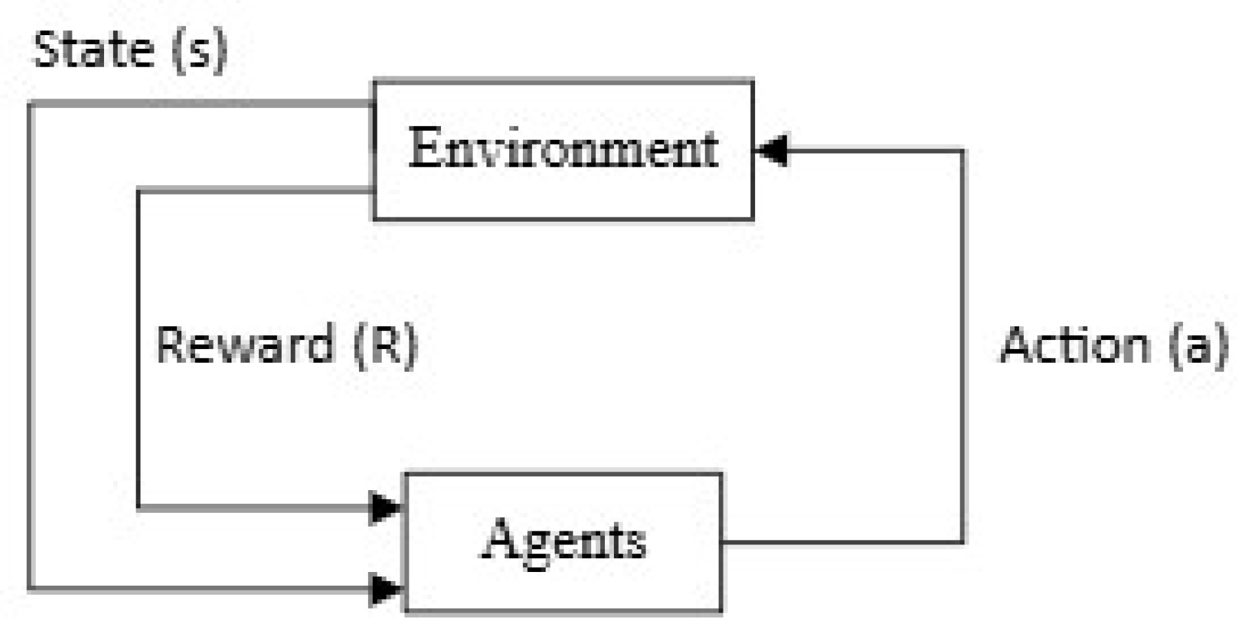
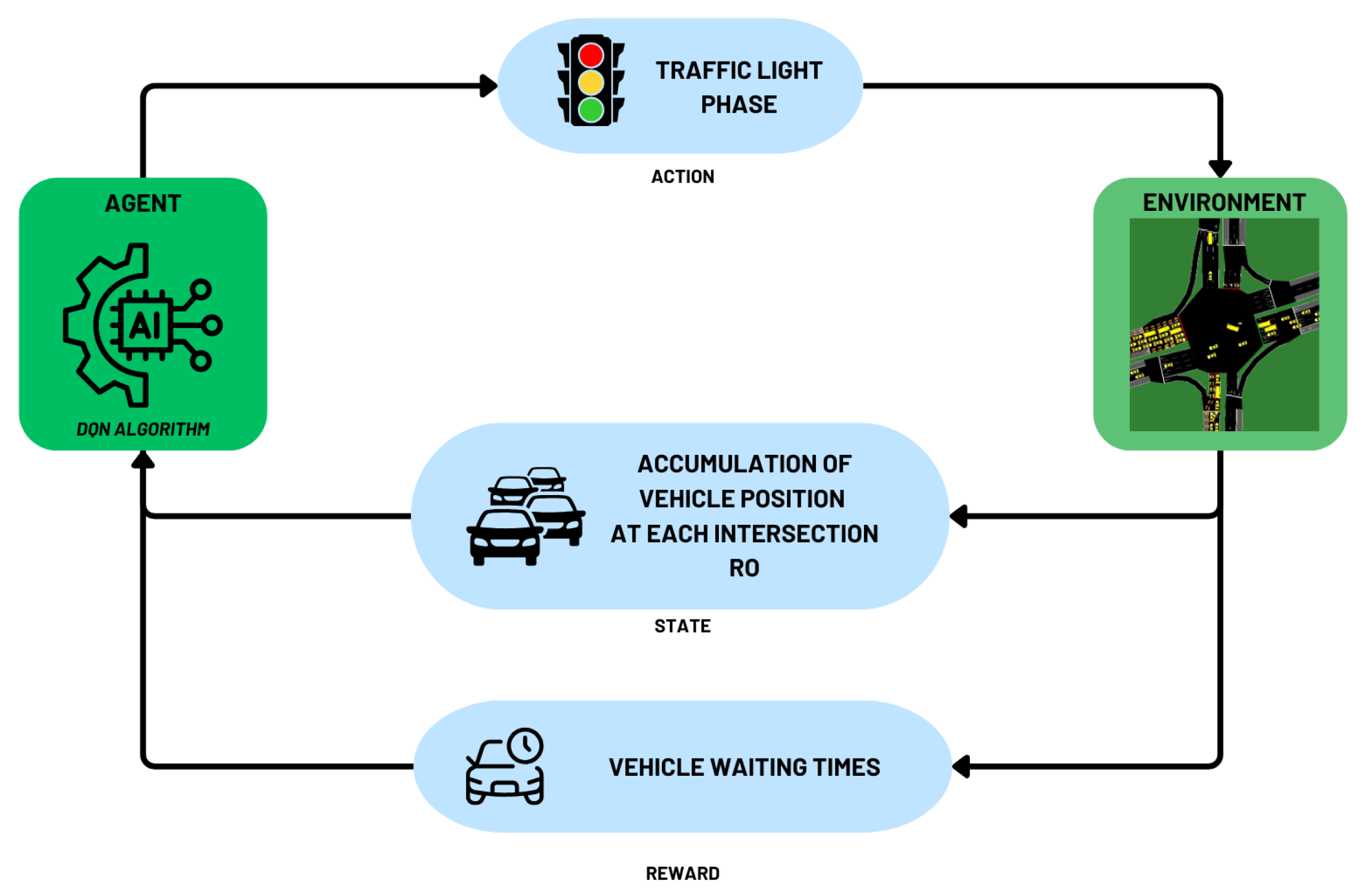
Based on several literature studies, the workflow or cycle of reinforcement learning is as follows, as shown in Figure 1.
In TSC, RL provides a flexible and adaptive approach to managing traffic flow. Traditional methods often rely on static rules or configuration on the traffic light settings [28], which may not effectively handle the ever-changing traffic conditions. RL systems, however, learn and adapt in real-time, optimizing traffic light phases based on current traffic data. This adaptability leads to reduced congestion, shorter wait times, and lower vehicle emissions.

2.4. Deep Q-Learning Network (DQN)

Recent research on RL for TSC has shown substantial promise in reducing urban traffic congestion through both simulations and real-world applications [17,29]. One notable study proposed a novel RL-TSC method that optimizes signal sets for each cycle length, effectively reducing average queue lengths by up to 11.4% in a real-world demonstration in Seoul, highlighting the practical applicability of such approaches [29].
Additionally, multi-agent deep Q-network (MADQN) approaches have been shown to reduce total travel time in high-traffic scenarios. This effectiveness was evidenced in a case study conducted in Sunway City, Malaysia, where the integration of MADQN significantly improved traffic flow compared to traditional methods [30].
Further investigation into Q-learning and DQN frameworks has revealed their effectiveness in improving safety and stability in dynamic traffic scenarios. Simulations with these frameworks indicated increased average velocities and reduced lane utilization rates, with DQN model enhancing average velocities with around 10% and decreasing lane utilization rates with around 30% in comparison to Q-learning. [31].
The implementation of Deep Q-network (DQN) as an adaptive traffic controller also has been tested in Jakarta, known for its congestion. DQN uses a reinforcement learning algorithm with an exponential reward function based on vehicle density distribution at intersections. The results show that DQN can increase vehicle throughput to 56,384 vehicles, outperforming conventional control methods like Webster, max-pressure, and uniform control. This increase indicates that DQN can reduce congestion and improve traffic productivity in Jakarta, making it a promising direction for future development of traffic control systems [32].
This research develops and evaluates a Deep Q-Network (DQN) model for optimizing traffic signal control at an isolated intersection in a partially observable environment with connected vehicles. The paper introduces a new state representation and reward function tailored for traffic signal control, along with a detailed network architecture and tuned hyper-parameters. The model’s performance is evaluated through numerical simulations across various scenarios, both under full detection conditions and partial detection with varying proportions of connected vehicles. The results are used to establish detection rate thresholds that yield acceptable and optimal performance. This research provides an effective solution for traffic signal optimization under limited detection conditions, leveraging connected vehicle technology [33].
Moreover, an improved DQN algorithm specifically designed for isolated intersections has shown substantial benefits. In a virtual simulation of a typical intersection in Xi’an, this method reduced vehicle waiting times by 26.7% and decreased queue lengths, thereby significantly enhancing intersection efficiency and overall road performance [34].
These findings collectively underscore the promise of DQN-based methods in effectively managing urban traffic congestion in discrete action, offering superior performance over traditional control methods and paving the way for more intelligent and adaptive traffic management systems [35].

2.4.1. DQN Formula

Q-value is calculated as Equation (1) as follows [31,36]
Q ( s t , a t ) Q ( s t , a t ) + α r t + 1 + γ max a Q ( s t + 1 , a ) Q ( s t , a t )
where:
  • Q ( s t , a t ) is the Q-value for state s t and action a t
  • α is the parameter that determines how much new data supersedes the existing information.
  • r t + 1 is The reward obtained after taking an action a t in a particular state is the reward received after taking action in state s s t .
  • γ is the discount factor that controls the importance of future rewards
  • s t + 1 is the state after taking action a t
  • max a Q ( s t + 1 , a ) is the maximum Q-value for state s t + 1 over all possible actions a
Equation (1) describes how the Q-value for a given state-action pair ( s t , a t ) is updated based on the observed reward r t + 1 and the maximum expected future reward max a Q ( s t + 1 , a ) . The learning rate α specifies how much new data replaces the existing information, while the discount factor γ specifies the significance of future payoffs.

2.4.2. Q-Value Calculation

The process of updating the Q-value Q ( s t , a t ) in Q-Learning begins by initializing the Q-value Q ( s , a ) for all state-action pairs ( s , a ) . This is commonly done using random values, frequently zero. Next, an action a t is selected in the current state s t using an epsilon-greedy policy, which strikes a balance between exploration (choosing random actions) and exploitation (choosing the best-known actions). After taking action a t in state s t , the reward r t + 1 and the new state s t + 1 are observed.
To update the Q-value, the highest Q-value for the new state s t + 1 across all possible actions a is calculated:
max a Q ( s t + 1 , a )
This step determines the maximum anticipated future reward that can be achieved from the new state s t + 1 . Afterward, the target value for the update is computed:
y t + 1 = r t + 1 + γ max a Q ( s t + 1 , a )
The target value y t + 1 represents the immediate reward plus the discounted maximum future reward, which serves as a reference for updating the Q-value for the current state-action combination.
The Q-value Q ( s t , a t ) is then updated by the Q-Learning update rule:
Q ( s t , a t ) Q ( s t , a t ) + α y t + 1 Q ( s t , a t )
By substituting the target value y t + 1 from the previous equation into the Q-Learning update rule, we get:
Q ( s t , a t ) Q ( s t , a t ) + α r t + 1 + γ max a Q ( s t + 1 , a ) Q ( s t , a t )
This update adjusts the Q-value Q ( s t , a t ) towards the target value, where the difference y t + 1 Q ( s t , a t ) is scaled by the learning rate α .
The entire process is repeated for each time step t + 1 , t + 2 , and t + n , until the Q-values converge, indicating the agent has learned the optimal policy.

3. Proposed System

3.1. Current Traffic Condition

The traffic light at the Kiaracondong intersection, particularly at the Soekarno Hatta-Ibrahim Adjie junction, has gained online notoriety due to its lengthy waiting times, earning nicknames like "the faith tester" and "Indonesia’s longest red light.". This intersection is often manually controlled by the Area Traffic Management System (ATCS) officers. This allows for the adjustment of light durations to alleviate congestion.
The Kiaracondong light cycle lasts 420 seconds, with 180 seconds for eastbound, 50 seconds for southbound, 110 seconds for westbound , and 80 seconds for northbound traffic. In cases of severe congestion, ATCS officers can extend green light durations to ease traffic. During peak morning hours (6:00-9:00 AM) and afternoon hours (3:00-6:00 PM), eastbound and westbound traffic is especially heavy, with more or less 50,000 vehicles in three hours. This leads to inevitable delays, as only 550 vehicles can pass through each 180-second cycle.
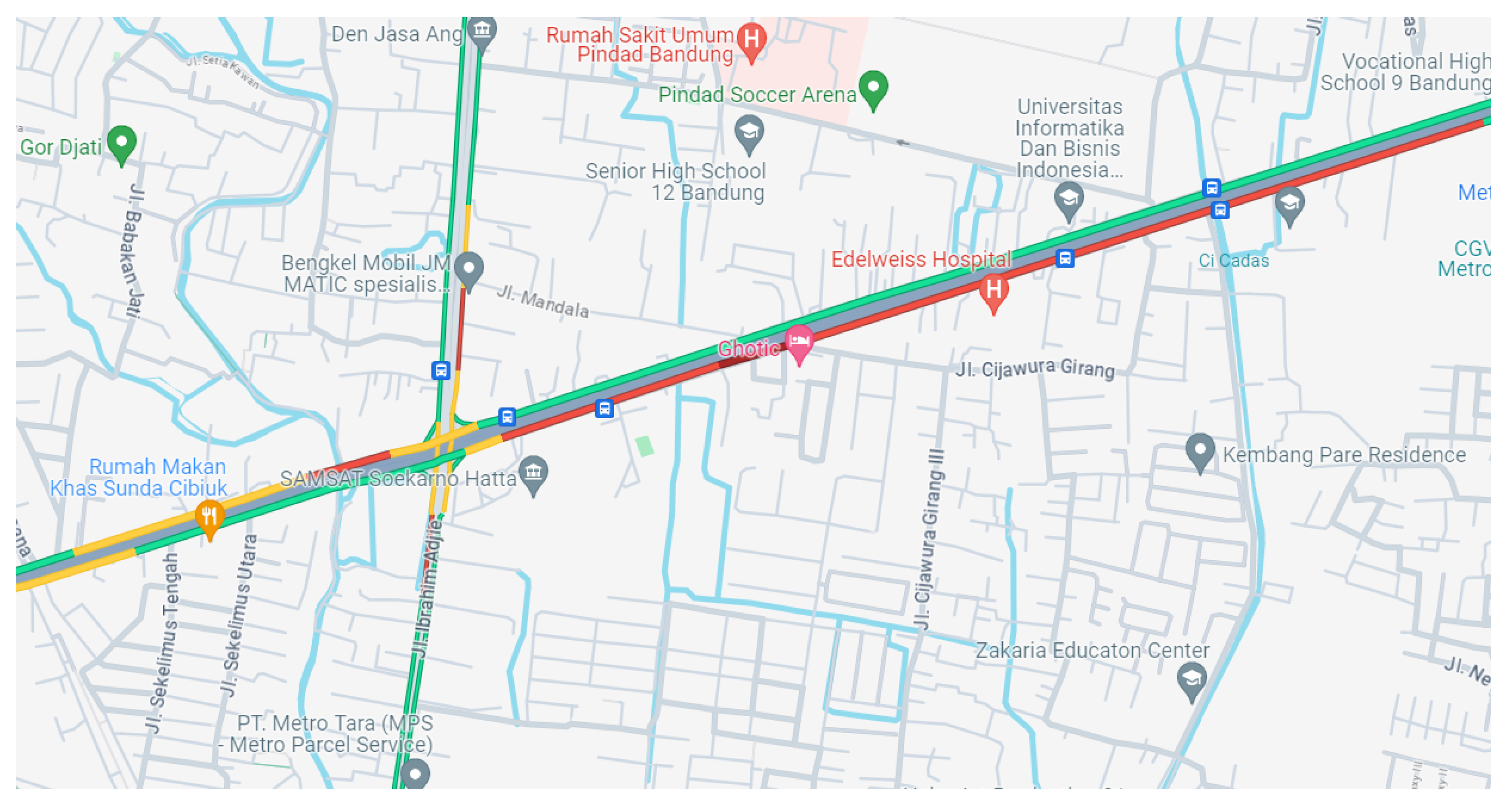
The intersection experiences the highest saturation levels as shown in Figure 2, necessitating intervention to manage the congestion. The Soekarno Hatta-Ibrahim Adjie junction is a critical meeting point for vehicles from East and South Bandung heading towards the city center, exacerbating traffic volumes. Furthermore, Bandung’s limited road capacity and high vehicle volume, particularly private cars, contribute significantly to daily traffic jams. The public is urged to use public transportation to mitigate congestion.
During rush hours, as illustrated in Figure 2, traffic congestion can extend up to 2 km on one leg of the intersection alone, indicating severe inefficiency in traffic management at this junction.
Due to this situation, this study investigates ways to reduce congestion. The system we propose will be explained in the System Design.

3.2. Research Gap

This research focuses on the Kiaracondong-Ibrahim Adjie intersection, addressing a critical research gap. Previous studies have not incorporated both simulations of exclusive two-wheeled vehicle lanes and Deep Q-Network (DQN) algorithms on the SUMO platform for this specific intersection. Earlier research has primarily employed alternative algorithms, such as multi-agent reinforcement learning (MARL) in Jakarta intersection [32], fuzzy logic [37], and traditional static control methods [28]. While these studies have made significant contributions, the integration of exclusive two-wheeled vehicle lanes and the application of DQN in traffic signal control within the SUMO simulation environment at the Kiaracondong-Ibrahim Adjie intersection remains unexplored. This study aims to fill this gap by investigating the impact of these additions on traffic efficiency and safety, providing a novel approach to urban traffic management.

3.3. System Design

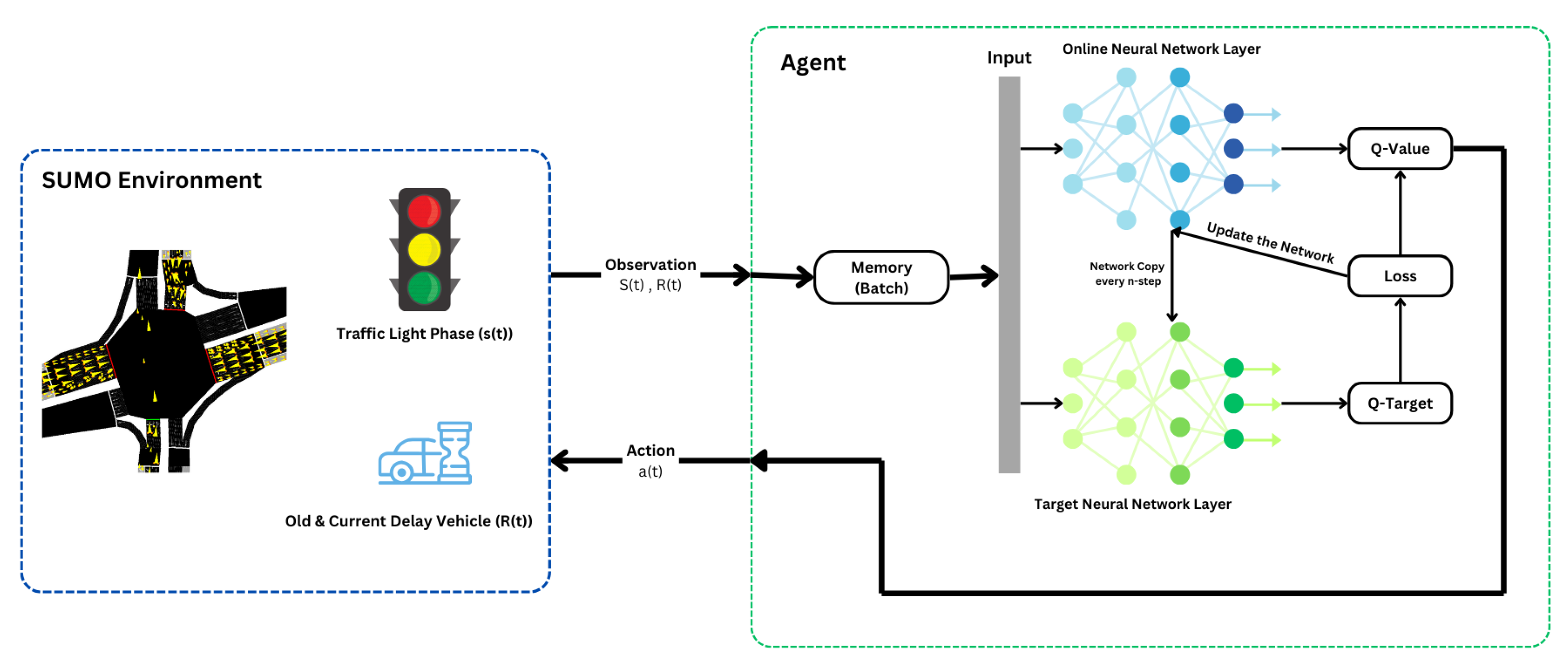
In this section, we developed a traffic light phase control system that implements additional two-wheeled vehicle lane and the Deep Q-Network (DQN) algorithm to optimize traffic distribution at intersections as shown on Figure 3. This system consists of several key components that work synergistically to achieve the goal of reducing congestion and improving traffic efficiency. The environment serves as a representation of a real-world intersection where vehicles move and are regulated by the traffic light system. Information about the position of vehicles on each road leading to the intersection is collected and used as a state representing the environmental condition at a given time.
Each state consists of spatial information about the position of vehicles in discrete cells dividing the roads leading to the intersection. The DQN algorithm receives this state and calculates the reward based on vehicle waiting times, which is used as a metric to evaluate the system’s performance in reducing congestion. This reward is used to update the algorithm’s policy, enabling it to take more optimal actions in the future.
The DQN algorithm generates actions in the form of traffic light phases (red, yellow, green) applied at the intersection. These actions aim to reduce vehicle waiting times and improve overall traffic flow. The system operates iteratively, where each action taken by the algorithm affects the environment, resulting in a new state and new reward for the next iteration.
The results of implementing this system demonstrate that using a reinforcement learning approach, traffic light phase control can be dynamically optimized according to real traffic conditions. This approach offers an adaptive and effective solution to traffic control problems, focusing on realism and ease of implementation, unlike previous methods that used information-rich states but were difficult to implement in reality.

3.3.1. Environment Design

This study involves configuring the SUMO (Simulation of Urban Mobility) environment to simulate traffic conditions at the Kiaracondong-Ibrahim Adjie intersection in Bandung, Indonesia. The simulation includes key parameters such as vehicle separation, simulation and data collection time steps, and lane widths to ensure realistic traffic modeling. Traffic light phase configurations are based on real-world data from ATCS Bandung, focusing on peak traffic periods to optimize flow. Additionally, dedicated exclusive two-wheeled vehicle lanes are designed according to Southeast Asian traffic standards.
SUMO Environment Configuration
Figure 4. The intersection of Kiaracondong and Ibrahim Adjie features a roundabout with four arms: west, east, north, and south. Dedicated exclusive two-wheeled vehicle lanes, marked in grey, provide a safe and continuous path through the roundabout, separate from 4-wheel or more vehicle lanes. Traffic signals at each entry point manage the flow, enhancing overall safety and efficiency.
Preprints 115069 g004
In this study, the configuration parameters of SUMO (Simulation of Urban Mobility) as shown on Table 4 were adjusted based on literature reviews to ensure realistic and relevant simulations of actual traffic conditions at the Kiaracondong-Ibrahim Adjie intersection. Initially, The minimum recommended separation between vehicles has been set at 1.5m. This parameter is essential to avoid collisions and ensure traffic safety, aligning with studies highlighting the importance of proper lane configurations for safety and efficiency [18].
Next, the simulation time step was set at every 1 second, allowing SUMO to update the state of vehicles and the environment responsively. This brief interval is essential for real-time TSC using RL algorithms [29]. For data collection, the interval was set at every 5 seconds. This interval ensures that minor changes in traffic conditions can be detected and evaluated promptly, supporting more accurate and in-depth analysis.
The best path selection was used to ensure that SUMO determines the most efficient vehicle paths based on current traffic conditions. This approach is important to create realistic and accurate simulations in measuring the impact of changes in traffic signal settings and two-wheeled vehicle lane configurations [30]. The regular lane width was set at 3.2m, reflecting the standard width for four-wheeled vehicle lanes, which is important for maintaining traffic safety and smooth flow.
Finally, the two-wheeled vehicle lane width was set at 3m. This determination is based on previous research that indicates the optimal width for exclusive two-wheeled vehicle lanes to reduce traffic density and improve safety [20,22]. The wider two-wheeled vehicle lane helps separate the flow of motorcycles from larger vehicles, reducing accidents and improving overall traffic efficiency.
With these configuration parameters, the SUMO simulation is expected to reflect the actual traffic conditions at the Kiaracondong-Ibrahim Adjie intersection, Bandung, Indonesia. This allows for accurate analysis of the impact of implementing exclusive two-wheeled vehicle lanes and Reinforcement Learning-based traffic signal control in reducing queue lengths and vehicle waiting times.
Traffic Light Phase Configuration
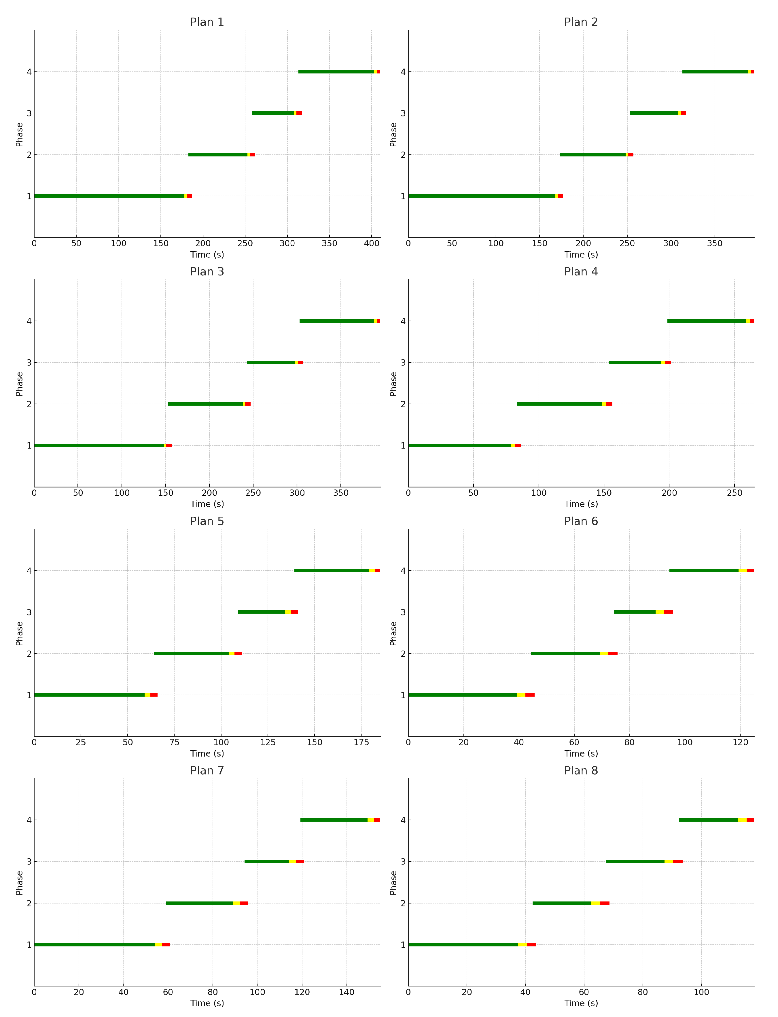
The traffic light plan data was collected from field configuration data provided by ATCS Bandung, which manages traffic control. There are 8 plans in operation for the traffic light settings at the Kiaracondong-Ibrahim Adjie intersection as shown on Figure 5. The plan changes are based on traffic density as agreed upon by ATCS Bandung. This study focuses on periods of maximum activity from early morning hours between 6:00 AM and 9:00 AM, as well as the late afternoon hours between 3:00 PM and 6:00 PM. During these periods, ATCS has determined that Plan 1 will be implemented from 6:00 AM to 9:00 AM, and Plan 3 will be applied from 3:00 PM to 6:00 PM. Consequently, the testing for both RL and Non-RL programs will employ Plan 1 and Plan 3.
The Table 5 illustrates the duration of green, yellow, and red phases for each plan and direction. It is important to note that the green light duration varies for each plan and direction, ensuring flexibility and adaptation to different traffic conditions. However, the yellow light duration is consistently set at 3 seconds and the red light duration is set at 2 seconds across all plans and directions. This consistency in the yellow and red light durations helps to maintain safety and predictability in traffic signal timings.
The Figure 5 is a visual representation of the traffic light duration data shown in Table 5. Each diagram in the image illustrates the traffic light duration plans for eight different plans (Plan 1 to Plan 8).
In each diagram, the horizontal axis represents time in seconds (s), while the vertical axis represents the traffic light phases. There are four phases represented by numbers 1 to 4 on the vertical axis. The green color on the lines indicates the duration of the green light, while the red color indicates the duration of the red light.

3.3.2. Agent Configuration

There are three elements agents are used in this section: state, action, and reward.
State, The representation of the state of a traffic intersection in terms of cell density using SUMO (Simulation of Urban Mobility) can be explained as follows. Initially, the simulation retrieves a list of vehicle IDs present in the environment using SUMO functions. For each vehicle, the position within its lane and the lane’s identifier are obtained. The lane position is then converted into a distance from the traffic light by subtracting the lane position from 750, which is considered the maximum length of the cell, indicating a highly congested road. This distance is used to map the vehicle to a specific cell representing a smaller segment of the road. The lane in which the vehicle is located is identified by checking the lane ID and mapping it to a corresponding lane group (north, west, south, east). Each lane group is assigned an index (0 to 3). The cell index is determined based on the distance from the traffic light, dividing this distance into several intervals. For example, a distance of 0-6m may be assigned cell index 0, a distance of 6-11m may be assigned cell index 1, and so on, up to a distance of 400-750m assigned cell index 9. The vehicle’s position is calculated by combining this lane group index with the cell index, resulting in a unique number within the range of 0 to 39. If the lane group is valid (with an index between 0 and 3), the position in the ’state’ array corresponding to the vehicle’s position is set to 1, indicating that this cell is occupied by a vehicle. The determination of the cell index lengths is the result of multiple experiments to achieve a satisfactory reward response, as shown in Figure 11. This function ultimately returns the ’state’ array, which indicates the cell density at the intersection and can be utilized for additional traffic analysis.
Figure 6. Cell Index Representation.
Preprints 115069 g006
Action, In the traffic simulation by using SUMO, actions act as simulation output that into the environment and will change the phase of traffic light continously. actions are selected and executed iteratively at each simulation step. The current state of the intersection is first collected to assess the positions and numbers of vehicles in various road segments. Based on this state, an action is chosen using an epsilon-greedy policy, which allows the model to either explore random actions or exploit the best action based on model predictions. If selected action is distinct from the preceding one, yellow light is initially activated to ensure a safe transition before switching to next green light. Green light duration is then determined, and the corresponding green light phase is activated. During each simulation step, reward is calculated based on the change in total vehicle waiting time at the intersection. Data regarding the state, action, reward, and next state is stored in memory to train the model at the end of the episode. This process enables the model to gradually learn to optimize traffic flow by reducing waiting times and queue lengths at the intersection.
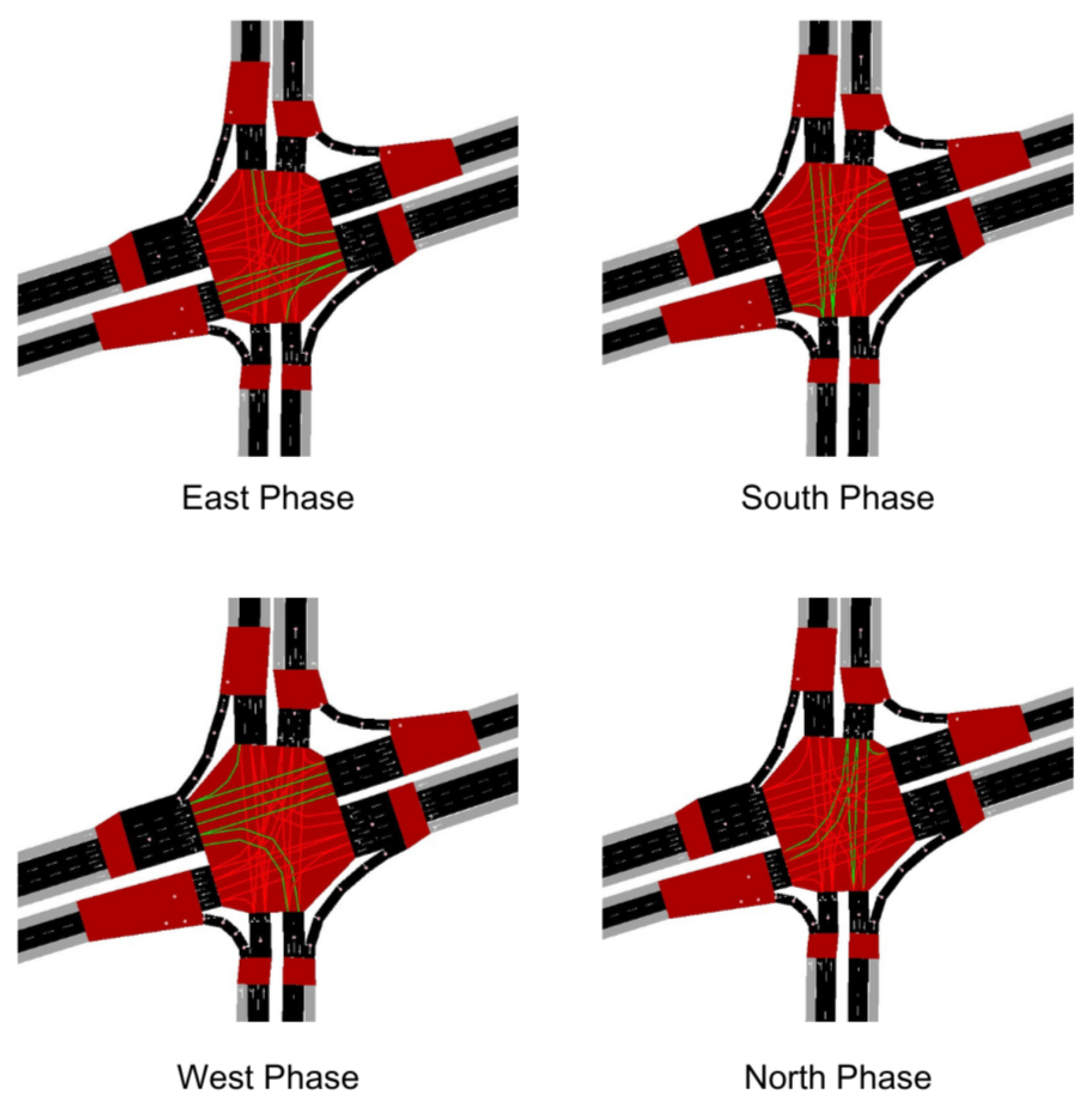
Figure 7. The Four Phases of Kiaracondong-Ibrahim Adjie Intersection.
Preprints 115069 g007
Reward, Reward calculation process is performed at each simulation step to assess the effectiveness of the actions taken. Total waiting time at the intersection is first collected, accounting for the time vehicles spend stopped on the incoming roads. The reward is determined as the distinction between the earlier total waiting time and the present total waiting time. Reduction in total waiting time results in a positive reward, indicating an improvement in traffic flow, while an increase leads to a negative reward. This reward reflects how well the action has mitigated congestion and enhanced traffic flow. This reward data, along with the state, action, and next state, is stored in memory to train the model at the end of the episode, enabling the model to learn from experience and improve future traffic light control decisions. The reward computation in the traffic simulation is based on total WT at the intersection. Key variables employed in the calculation are described as follows:
  • W t : Total cumulative waiting time at time t.
  • W t 1 : Total cumulative waiting time at time t 1 .
  • r t : Reward at time t.
The reward on each simulation step is determined by the change in the total waiting time from the past time step ( t 1 ) to the present time step (t):
r t = W t 1 W t
If the waiting time decreases, fewer vehicles are waiting. then r t will be positive, indicating that the action taken is beneficial. Conversely, if the cumulative waiting time increases, r t will be negative, indicating that the action taken is detrimental.
The accumulated negative reward over one episode is calculated by summing all the negative rewards.
Let R neg be the accumulated negative reward over one episode, then:
R neg = t = 1 T min ( r t , 0 )
where T is steps for one episode. State of the intersection is represented as a vector of cell densities, where each cell corresponds to a specific segment of the incoming lanes. The action space consists of different traffic light phases that can be activated, each corresponding to a specific direction (e.g., east, west, north, south).

4. Experiments

4.1. Two-Wheeled Vehicle Lane Configuration

The design of the two-wheeled vehicle lane in this study is grounded in prior research that emphasizes the road configurations in various Southeast Asian countries. This research indicates that the recommended width for exclusive two-wheeled vehicle lanes should be between 1m and 3m, depending on the specific traffic conditions prevalent in the region. Southeast Asia, with its unique traffic patterns and high volume of two-wheeled vehicles, necessitates such dedicated lanes to ensure safety and efficiency [23].
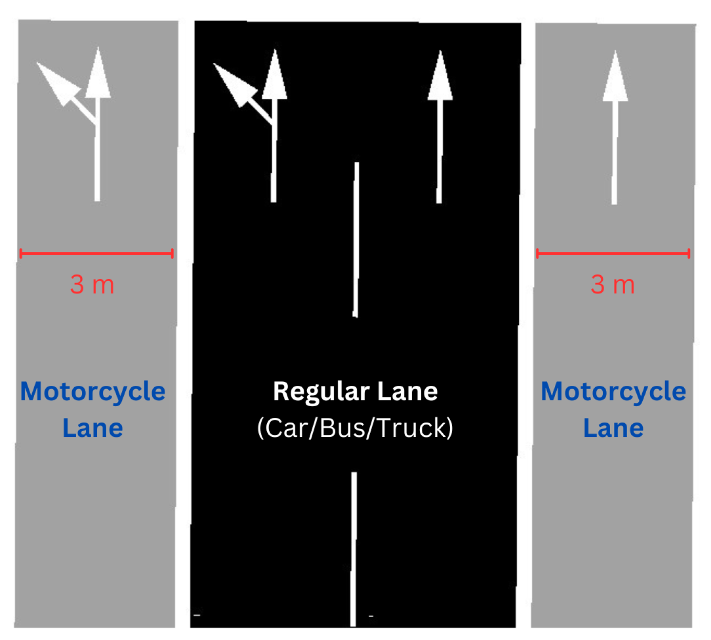
In this study, we have opted for the maximum width of 3m as the standard as shown on Figure 8. This decision is particularly influenced by the traffic conditions at the Kiaracondong-Ibrahim Adjie intersection, a critical arterial road known for its extremely high traffic density, in this case more than 2000 motorcycle per hour passed the intersection, so we used 3m width for the configuration [23]. This intersection frequently experiences long queues and significant congestion, which can severely impact overall traffic flow and safety. By adopting the maximum lane width, we aim to accommodate the heavy volume of motorcycles and other vehicles more effectively, thereby reducing congestion and enhancing the overall movement of traffic. The broader lane provides ample space for motorcycles to maneuver safely, even during peak traffic hours, which is essential for minimizing accidents and improving traffic efficiency in one of the busiest areas of the city.
In Figure 8, the configuration of the exclusive two-wheeled vehicle lanes has been carefully designed to ensure optimal traffic flow and safety. Each lane is precisely set to a width of 3m. The northern, western, and eastern road, are main arterial roads, there are two two-wheeled vehicle lanes located on both the right and left sides. This dual-lane setup accommodates the high traffic volume typical of these primary routes. In contrast, the southern side, being a secondary arterial road, features only a single two-wheeled vehicle lane due to its lower traffic capacity. This strategic arrangement of lanes, tailored to the specific demands of each road, not only maximizes the efficiency of motorcycle traffic but also enhances overall road safety by providing ample space for maneuvering.

4.2. DQN Implementation

Figure 9 is the integration of a SUMO environment with a reinforcement learning (RL) agent to optimize traffic light control. In the SUMO environment, the traffic light phase s t and vehicle delay r t are observed, representing the state and reward, respectively. The RL agent receives these observations, processes them through an online neural network to estimate Q-values, which predict future rewards for specific actions, and updates these estimates using a target neural network for stability. The agent’s experiences, which include various states, actions, rewards, and the resulting states, are saved in a memory buffer. The agent’s experiences are then sampled in batches to train the neural network.
The loss is calculated as the difference between the predicted Q-values and the target Q-values, and this loss is backpropagated to improve the network’s accuracy. The agent then selects the best action a t relying on the Q-values, adjusting the traffic light phases to minimize vehicle delays and improve queue length and waiting times at the intersection (environment). This continuous feedback loop allows the RL agent learning and applying efficient traffic management strategies, showcasing potential of RL in enhancing urban traffic systems.
Table 6. Terminology List.
Parameter Name Symbol
Current State s t
Next State s t + 1
Action a t
Reward r t + 1
Learning Rate α
Discount Factor γ
Q-value Q ( s , a )
QL Queue Length
WT Waiting Times
DQN Deep Q-learning Network
In a Q-Learning program, several crucial parameters are used to effectively train an agent within a dynamic environment. The Current State ( s t ) represents the agent’s state within the environment at a spesific time t. This state provides the agent with the necessary information about the environment, which is essential for decision-making. After the agent’s action, the environment transitions to Next State ( s t + 1 ), reflecting state of the environment after the action has been taken. The action taken by the agent, referred to as Action ( a t ), is determined based on a policy that the agent follows, aiming to maximize its cumulative reward.
The Reward ( r t + 1 ) is immediate feedback received by the agent upon shifting to next state, offering a measure of the effectiveness of the action taken. This reward guides the agent’s learning process, assisting it in discerning which actions lead to favorable outcomes. To update its knowledge, the agent employs the Learning Rate ( α ), a parameter that dictates the speed at which new information is incorporated into the existing knowledge base. A higher learning rate implies rapid adaptation to new experiences, while a lower rate results in slower adaptation.
A critical parameter is Discount Factor ( γ ) that influences the agent’s decision-making process by determining the significance of future rewards. As the discount factor approaches 1, the agent places greater emphasis on future rewards, encouraging long-term planning. Conversely, a lower discount factor prioritizes immediate rewards. The Q-value (Q(s,a)) is a function that estimates the expected utility of performing a specific action in a given state, providing guidance to the agent in selecting actions that maximize its long-term cumulative reward.
Collectively, these parameters enable the Q-Learning algorithm to iteratively refine the agent’s policy. The agent learns from each interaction with the environment, updating its Q-values to reflect the estimated benefits of actions in various states. Over time, this process allows the agent to develop an optimal policy that maximizes its total reward, thereby navigating the environment both efficiently and effectively. This iterative learning approach is foundational to the success of reinforcement learning techniques in dynamic and uncertain environments.

4.3. SUMO Simulation

SUMO is a traffic simulation tool known for its flexibility, detailed modeling, and real-time capabilities, making it ideal for testing traffic management and vehicular communication strategies. Two main files are essential for SUMO simulations:
  • Network file (“.net.xml”): Describes the road network, including roads, intersections, lanes, and speed limits.
  • Routes file (“.rou.xml”): Defines vehicle routes, including types, routes, and departure times.
These files are referenced in a configuration file (“.sumocfg”), which sets the simulation’s parameters. Furthermore, programming languages can interface with SUMO via its TraCI (Traffic Control Interface) API, allowing for real-time control and the integration of machine learning algorithms. This enhances traffic management, reduces congestion, and enables the testing of autonomous vehicle systems.
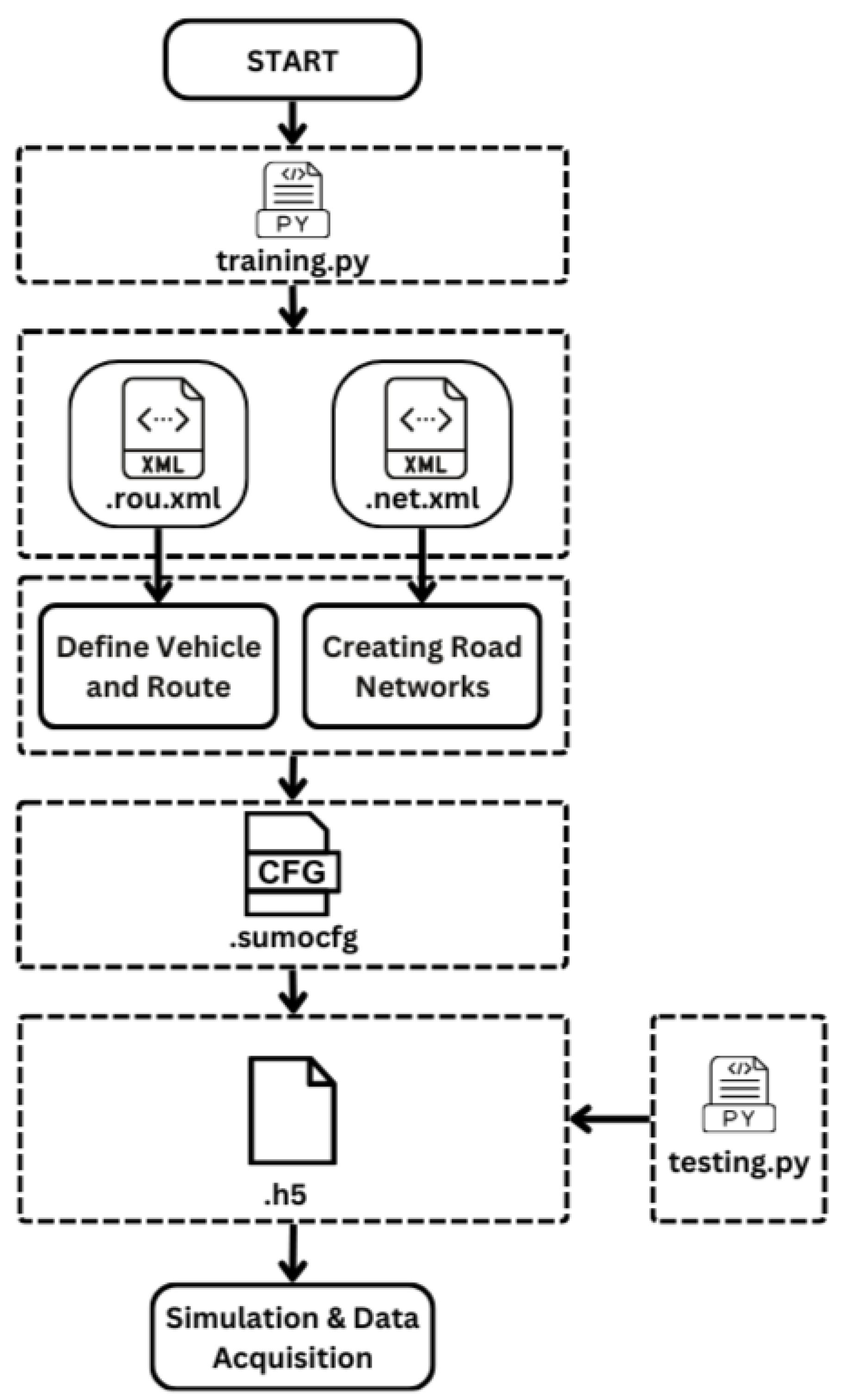
Flow of Simulation on Figure 10 explains the steps involved in setting up and running a simulation using SUMO. First, the process begins by running the Python script training.py, which works with existing setup files rou.xml and net.xml. The rou.xml file defines the vehicles and their routes within the simulation, including vehicle types, quantities, departure times, and routes. Meanwhile, the net.xml file describes the road network, including the layout of streets, intersections, traffic lights, and other infrastructure.
Next, these files are used to define the simulation configuration in the .sumocfg file. The SUMO configuration file (.sumocfg) sets the overall parameters for the simulation, such as the simulation duration, step length, and the files to be used. Once the configuration is complete, the simulation is run based on these settings, and various data points such as vehicle positions, speeds, and waiting times are collected during the simulation. The collected data is then stored in an .h5 file, which is suitable for storing large datasets.
The final step involves data analysis using another Python script, testing.py, which is used to analyze the simulation results. This script may perform various analyses, including performance metrics, visualization, or validation against real-world data. Thus, this process as a whole describes the workflow for setting up, running, and analyzing a traffic simulation using SUMO.

4.4. DQN Training Process

4.4.1. DQN Training Configuration

Based on Figure 5, the plans executed during rush hours are Plan 1 and Plan 3. These plans are implemented to manage the high traffic volumes typically experienced during these times. The specific durations for each phase of the traffic signals—green, yellow, and red—are critical for ensuring smooth traffic flow and minimizing congestion. The detailed durations for each direction (East, West, South, and North) and for each type of phase are summarized in Table 5. The table offers a concise depiction of the timing settings employed to enhance traffic control at the Kiaracondong-Ibrahim Adjie intersection during high-traffic periods. This information will be utilized for both training and evaluation purposes.
RL training is a process in where an agent learns to make an best decisions through action with the environment. In the context of traffic management, this agent aims to reduce vehicle wait times at intersections by optimizing traffic light phases. The RL agent is trained to take actions based on the present state and receive feedback as rewards, reflecting how well these actions achieve the desired goals. In this study, data for training RL was obtained from raw datasheets of the ATCS Bandung city over three months. This data includes the number of vehicles coming from the west, east, north, and south. The training process was conducted over 100 episodes with the following parameters, as shown in Table 7.
Number of layers: This parameter refers to the number of hidden layers in the neural network used for training the reinforcement learning model. More layers can capture more complex patterns, but they also require more computational resources.
Layer width: This indicates the number of neurons in each hidden layer of the neural network. A wider layer can capture more features of the input data, improving the model’s learning capacity.
Batch size: The batch size is the number of training samples used in one iteration before updating the model parameters. A larger batch size can lead to more stable updates, but it requires more memory.
Learning rate: The learning rate is a hyperparameter that controls how much to change the model in response to the estimated error each time the model weights are updated. A smaller learning rate means the model is updated slowly, which can lead to better convergence but requires more training epochs.
Training epochs: The number of epochs is the number of complete passes through the entire training dataset. More epochs allow the model to learn better, but too many can lead to overfitting.
epsilon start: This is the initial value of epsilon in epsilon-greedy policy, which controls the exploration-exploitation trade-off in reinforcement learning. A higher epsilon encourages exploration.
epsilon end: This is the minimum value of epsilon to which it decays. Lower epsilon encourages exploitation, where the agent uses its learned policy more than exploring new actions.
epsilon decay: This parameter determines the rate at which epsilon decreases from epsilon start to epsilon end. A slower decay means the agent will explore more before converging to a stable policy.
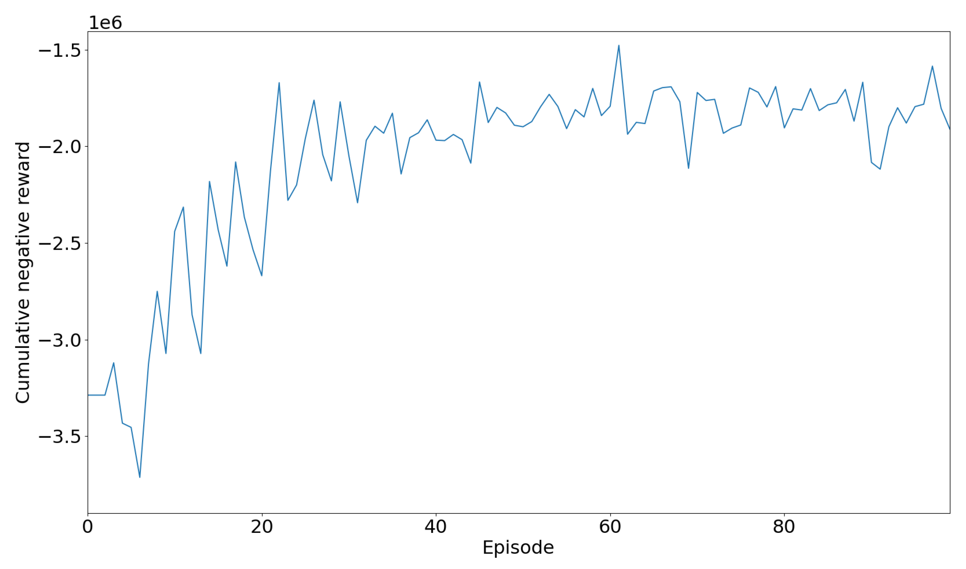
The parameters in Table 7 were obtained from an experimental with change the parameters one by one until achieving a positive trend reward output as shown on Figure 11.
Figure 11. Training Reward Plot.
Preprints 115069 g011

4.4.2. Training Result

Figure 11 illustrates the cumulative negative reward obtained during the training process of a Deep Q-Network (DQN) algorithm over a series of episodes. Initially, the cumulative negative reward exhibits a marked increase, indicative of the agent’s initial struggle to perform optimally as it explores the action space and learns the environment dynamics. This phase is characterized by substantial negative rewards, reflecting the agent’s trial-and-error learning approach.
As training progresses, the cumulative negative reward begins to oscillate, showing significant fluctuations around a gradually increasing trend. This behavior is emblematic of the exploration and exploitation trade-off inherent in RL algorithms, where the agent oscillates between trying new actions and exploiting known strategies that yield better outcomes. Towards the later episodes, the cumulative negative reward trend appears to stabilize slightly, suggesting that agent is learning in avoiding actions and resulting in high negative rewards and is approaching a more optimal policy. However, the persistent fluctuations indicate that the learning process is not entirely stable, and further training or hyperparameter tuning may be required to achieve more consistent performance.
The trend analysis reveals that during the initial episodes (0 to around 20), the cumulative negative reward increases significantly, reflecting poor performance as the agent explores the environment. From episode 20 to around 60, the reward fluctuates but generally trends upwards, indicating that the agent’s performance is improving with experience. After episode 60, the fluctuations continue, but the trend stabilizes, hinting at some level of convergence.
The significant reward fluctuations, particularly in the middle episodes, can be attributed to the agent balancing exploration of new actions and exploitation of learned policies. These fluctuations underscore the dynamic nature of the learning process in DQN algorithms.
In terms of performance evaluation, the overall increase in the cumulative negative reward suggests that the agent is learning to reduce negative outcomes over time. The stabilization towards the later episodes indicates that the agent is approaching an optimal policy, although further training might be necessary to achieve more consistent performance. This comprehensive analysis of the DQN algorithm’s learning trajectory highlights both the progress made and the challenges remaining in optimizing the agent’s performance.
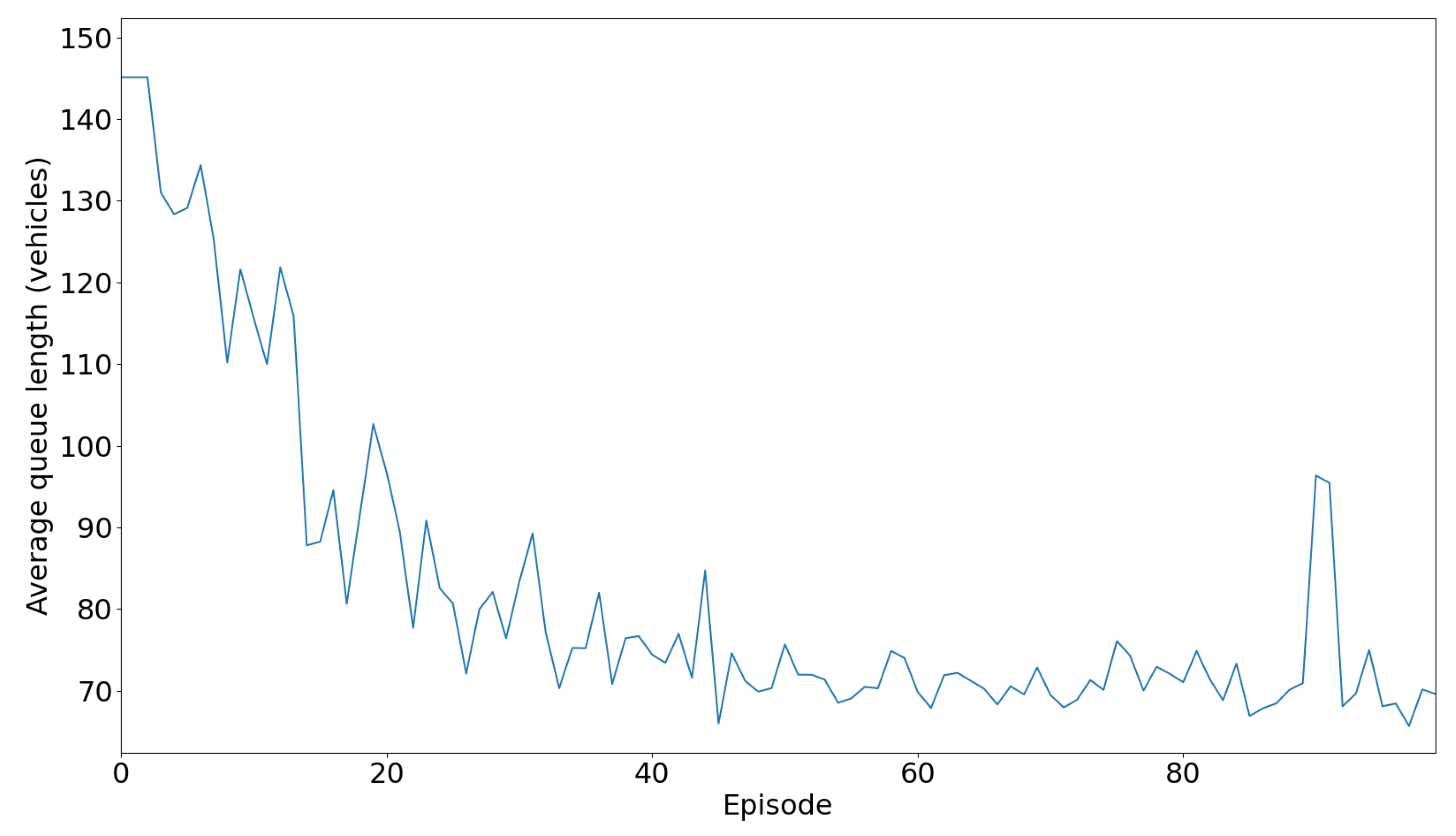
Figure 12 illustrates the average length of queue at traffic intersections over a series of episodes during the training of a Deep Q-Network (DQN) algorithm. Initially, the average queue length is high, starting at approximately 150 vehicles and gradually decreasing to around 90 vehicles within the first 20 episodes, reflecting the agent’s initial inefficiency in managing traffic.
As training progresses, between episodes 20 and 60, the average queue length continues to decrease and fluctuates around 80 vehicles, indicating the agent’s improvement in traffic signal control. After episode 60, the average queue length stabilizes around 70-80 vehicles, with occasional spikes, suggesting that the agent has developed a more consistent and effective policy.
The fluctuations in average queue length, especially in the initial and middle episodes, highlight the agent’s exploration and exploitation process, experimenting with different signal timings to find the most effective approach.
This performance evaluation aligns with the cumulative negative reward analysis. The high average queue length in the initial episodes correlates with high negative rewards, indicating initial inefficiency. As training progresses, the decrease in average queue length and negative rewards suggests the agent’s improved traffic management. Stabilization in the later episodes corresponds with a stable cumulative negative reward trend, indicating the agent’s convergence towards an optimal policy.
Overall, the DQN algorithm effectively learns and optimizes traffic signal control strategies over time, leading to reduced queue lengths and negative rewards, improved traffic flow, and minimized congestion.
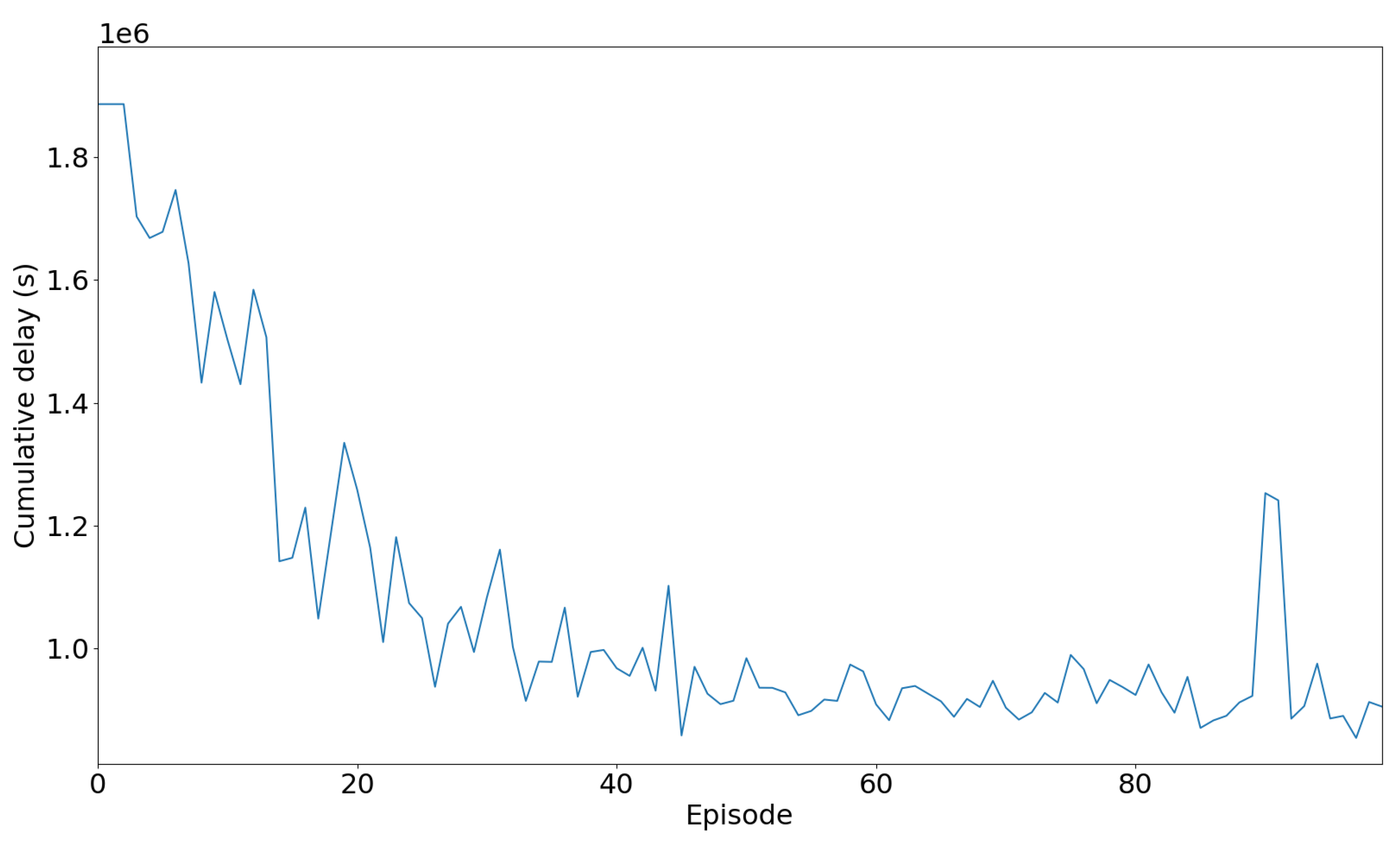
Figure 13 illustrates the cumulative delay in seconds experienced by vehicles over a series of episodes during the training of a Deep Q-Network (DQN) algorithm. Initially, the cumulative delay is high, starting at around 1.8 million seconds, indicating significant waiting times for vehicles. As the training progresses, there is a noticeable and substantial decrease in cumulative delay, demonstrating the DQN agent’s learning and adaptation to optimize traffic flow. By the later episodes, the cumulative delay stabilizes around 1 million seconds, with only minor fluctuations. This decrease and eventual stabilization in cumulative delay indicate that the agent has developed an effective strategy for managing traffic signals, leading to more efficient traffic flow and significantly reduced vehicle waiting times. Overall, the DQN algorithm successfully learns to minimize traffic delays, showing clear improvements in traffic management efficiency over the training period.

4.5. DQN Testing Process

The next step involves testing the performance of the trained RL model using the generated training.h5 file from training process. Testing phase is to assess the RL model’s effectiveness in reducing vehicle the WT value and the QL value at intersections compared to a non-RL system. During testing, data on QL and WT are collected from all directions of the intersection. QL and WT for car lanes and two-wheeled vehicle lanes are calculated separately to allow for a detailed comparison between the RL and non-RL systems. The QL value is measured by number of vehicles waiting at each intersection approach, while WT value is the total time vehicles spend in the queue before passing through the intersection. This data is continuously gathered over the testing period to provide comprehensive information.
Testing phase is critical to evaluate the functioning of trained RL-model, encapsulated in the training.h5 file, which represents the culmination of the previous training process. This phase aims to assess the model’s efficiency in controlling traffic signals and minimizing vehicle delays at intersections compared to a system that does not utilize reinforcement learning.
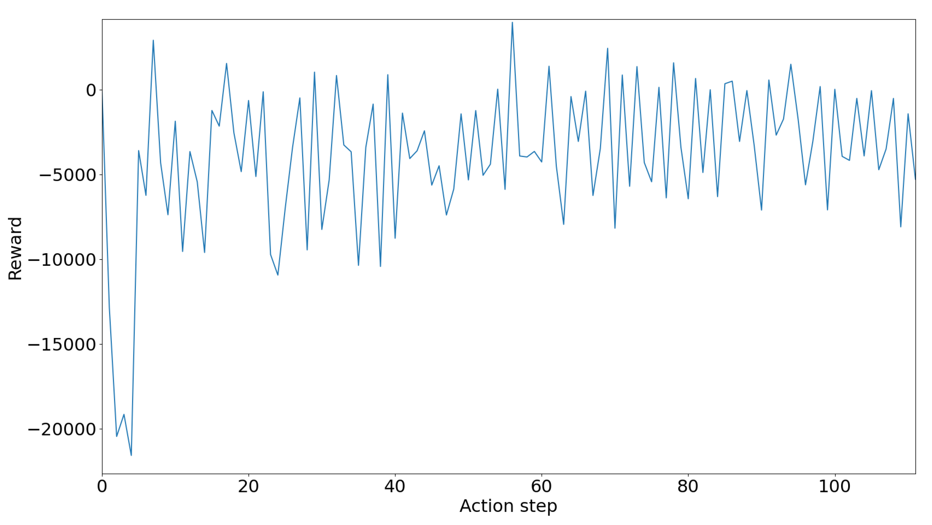
The provided graph on Figure 14 illustrates the reward trend over a series of action steps during the testing phase. Initially, the reward starts at a significantly negative value, around -20,000, indicating some suboptimal actions as the model adjusts to the testing environment. As the action steps progress, the rewards fluctuate considerably, reflecting the dynamic nature of traffic conditions and the RL model’s responses to these variations. Despite these fluctuations, the overall reward trend stabilizes closer to zero as the number of action steps increases. This stabilization suggests that the RL model is generally performing better, learning to optimize traffic signals effectively, and reducing wait times more consistently.
The fluctuating but generally stabilizing rewards indicate that the RL model, trained using the training.h5 file, can manage traffic signals effectively. The initial negative rewards are part of the adjustment process, and as the model continues to take actions, it adapts to the traffic conditions, resulting in more optimal traffic management. In summary, the testing results demonstrate that the RL model can improve traffic light management efficiency, as evidenced by the reward trends. Despite some initial and occasional suboptimal actions, the model generally converges towards better performance, reducing vehicle wait times and managing traffic flow more effectively. These insights are crucial for comparing the RL model’s performance against a non-RL system and understanding the potential benefits of implementing RL-based traffic management in real-world scenarios.

5. Results & Discussion

5.1. Experiments Result

There are ten parameters used in this study to collect data, with each parameter representing a different condition and type of data:
  • QL-Reg-Current
  • QL-Reg-No RL
  • QL-Reg-With RL
  • QL-ML-No RL
  • QL-ML-With RL
  • WT-Reg-Current
  • WT-Reg-No RL
  • WT-Reg-With RL
  • WT-ML-No RL
  • WT-ML-With RL
The explanation of each subparameter of these parameters is provided in Table 8.
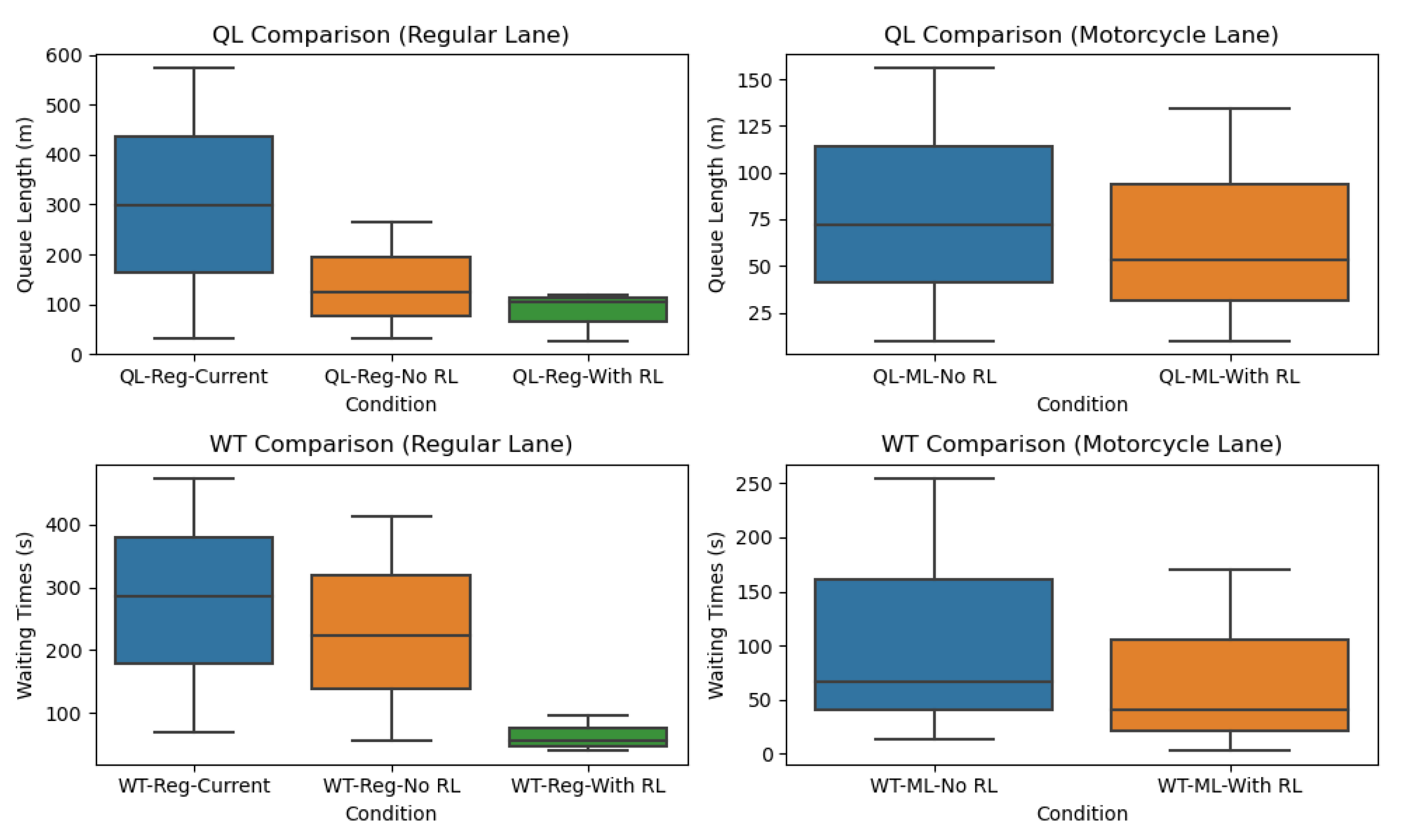
During the testing process, ten parameters previously explained were used. These parameters were analyzed to observe the impact of implementing two-wheeled vehicle lanes and the DQN algorithm compared to previous conditions. The analysis not only examined changes from the current state to the final state but also compared the current conditions with conditions after adding two-wheeled vehicle lanes without the DQN algorithm. Additionally, comparisons were made between two-wheeled vehicle lanes without DQN and with DQN, as well as the current conditions with those incorporating both two-wheeled vehicle lanes and RL as shown on Figure 15.
The box plots in Figure 15 provide a detailed comparative analysis of Queue Length (QL) and Waiting Times (WT) across two different lane types: Regular Lane and two-wheeled vehicle lane, under varying conditions. These plots enable a deeper understanding of the traffic dynamics and the effect of reinforcement learning (RL) control on traffic management.
The first subplot (QL-Comparison in Regular Lane) focuses on the queue lengths in regular lanes under three specific conditions. The data indicates that the highest queue lengths are observed under current conditions, labeled as QL-Reg-Current, with an average queue length of 297.9m, a minimum of 30m, and a maximum of 574m. Comparatively, when reinforcement learning control is not applied, marked as QL-Reg-No RL, there is a noticeable decrease in queue lengths to an average of 124.9m, with a minimum of 30m and a maximum of 264m. This scenario depicts the traffic situation where traditional traffic management techniques are employed, excluding advanced RL methods. The shortest queue lengths are achieved with RL control using Deep Q-Network (DQN), designated as QL-Reg-With RL, with an average of 104.58m, a minimum of 27m, and a maximum of 119.4m. This condition demonstrates the effectiveness of RL in optimizing traffic flow and reducing congestion significantly in regular lanes. The RL approach leads to an average queue length reduction of 193.32m compared to the current conditions and 20.32m compared to the traditional methods.
The second subplot (QL-Comparison in two-wheeled vehicle lane) presents the comparison of queue lengths in two-wheeled vehicle lanes under two conditions. Without the application of RL control, referred to as QL-ML-No RL, longer queue lengths are evident, with an average of 72m, a minimum of 10m, and a maximum of 156m. This situation reflects the conventional traffic management approach that does not utilize advanced RL techniques. In contrast, when RL control using DQN is implemented, indicated as QL-ML-With RL, there is a substantial reduction in queue lengths to an average of 53m, a minimum of 10m, and a maximum of 134m. This outcome showcases the capacity of RL to efficiently manage motorcycle traffic, thereby minimizing delays and enhancing the overall traffic flow. The RL approach results in an average queue length reduction of 19m.
The third subplot (WT-Comparison in Regular Lane) focuses on waiting times in regular lanes under three different conditions. The current waiting times, marked as WT-Reg-Current, are the longest, with an average waiting time of 284.85 seconds, a minimum of 70 seconds, and a maximum of 474.3 seconds, highlighting the inefficiencies in the existing traffic management system. When RL control is not applied, represented by WT-Reg-No RL, the waiting times decrease to an average of 223.4 seconds, with a minimum of 55 seconds and a maximum of 414 seconds, showing some improvement over the current conditions but still lacking the efficiency of RL methods. The shortest waiting times are recorded under RL control using DQN, labeled as WT-Reg-With RL, with an average of 55.6 seconds, a minimum of 40 seconds, and a maximum of 95 seconds. This scenario underscores the superior performance of RL in reducing waiting times, thereby improving the overall traffic efficiency in regular lanes. The RL approach leads to an average waiting time reduction of 229.25 seconds compared to the current conditions and 167.8 seconds compared to the traditional methods.
The fourth subplot (WT-Comparison in two-wheeled vehicle lane) compares the waiting times in two-wheeled vehicle lanes under two conditions. Longer waiting times are observed without RL control, indicated as WT-ML-No RL, with an average of 66.62 seconds, a minimum of 14 seconds, and a maximum of 255 seconds. This scenario reflects the limitations of traditional traffic management systems in handling motorcycle traffic efficiently. Conversely, the implementation of RL control using DQN, marked as WT-ML-With RL, results in decreased waiting times to an average of 40 seconds, a minimum of 3 seconds, and a maximum of 170 seconds. This demonstrates the effectiveness of RL in optimizing the flow of motorcycle traffic, significantly reducing delays. The RL approach results in an average waiting time reduction of 26.62 seconds.
These detailed numerical reductions highlight the impact of RL in managing traffic more effectively compared to current and traditional traffic management systems.
Overall, the application of reinforcement learning control using DQN proves to be highly effective in reducing both queue lengths and waiting times in both regular and two-wheeled vehicle lanes. The analysis reveals that the current conditions in regular lanes exhibit the highest queue lengths and waiting times compared to other conditions, emphasizing the need for advanced traffic management solutions. In two-wheeled vehicle lanes, RL control shows a marked improvement in managing traffic flow, highlighting its potential in enhancing traffic efficiency.
The box plots provide a summary of the overall QL and WT at all intersection approaches. These plots, lower boundary represents the minimum values (min), the upper boundary denotes the maximum values (max), and the body of the box plot illustrates the average values (mean). This detailed analysis offers a comprehensive understanding of traffic conditions and highlights the significant improvements achieved through the application of reinforcement learning control. Figure 15 clearly demonstrates the substantial impact of reinforcement learning control on enhancing traffic flow efficiency.
The percentage change is calculated using the following formula:
Percentage Change = V f V i V i × 100
where:
  • V i represents the initial average value.
  • V f denotes the final average value.
By using Equation (8), the summarized results can be effectively presented in the form of a table as follows:
Overall, as shown in Table 9, Table 10, Table 11, Table 12, Table 13, Table 14, Table 15 and Table 16. The implementation of DQN and two-wheeled vehicle lane consistently reduced both queue lengths (QL) and waiting times (WT) across all conditions.

5.2. Discussion

The experiment results demonstrate a significant reduction in both queue lengths and waiting times under conditions where Reinforcement Learning (RL) is applied, specifically using the Deep Q-Network (DQN) algorithm, in both regular and two-wheeled vehicle lanes. These findings can be explained scientifically through several key mechanisms.
The DQN algorithm is designed to learn optimal traffic signal control strategies by continuously interacting with the traffic environment. It employs a reward-based system to maximize traffic flow and minimize congestion. By leveraging this approach, DQN dynamically adjusts traffic signal timings to respond to real-time traffic conditions, leading to more efficient traffic management. This improvement is achieved through state-action mapping, where DQN maps current traffic conditions to traffic signal adjustments via a neural network. This allows the model to predict the most effective actions to take, significantly reducing the average queue length in regular lanes from 297.9m to 104.58m, a decrease of 64.89%. Additionally, the introduction of exclusive two-wheeled vehicle lanes segregates motorcycles from regular lanes, reducing overall congestion in both lane types. RL further optimizes the flow within these exclusive two-wheeled vehicle lanes, decreasing average queue lengths from 72m to 53m, a reduction of 26.39%.
Regarding waiting times, the DQN algorithm optimizes the duration of green, yellow, and red lights based on real-time traffic data. This dynamic adjustment minimizes waiting times by reducing idle periods at intersections, leading to a substantial decrease in average waiting times in regular lanes from 284.85 seconds to 55.6 seconds, an 80.49% reduction. Unlike static traffic control systems, RL adapts in real-time to changing traffic patterns. This continuous learning process ensures that traffic signals are always set to the most efficient timings, accommodating fluctuations in traffic volumes and patterns. This adaptability results in a reduction of average waiting times in two-wheeled vehicle lanes from 66.62 seconds to 40 seconds, a 39.96% decrease. The advantage of RL over traditional methods lies in its ability to improve through experience. By interacting with the traffic environment, the DQN algorithm learns from previous actions and outcomes, refining its strategy over time to achieve better results, leading to more efficient traffic signal control and reduced congestion.
The DQN algorithm utilizes a neural network to approximate the optimal policy for traffic signal control, relying on a reward function that penalizes long queues and waiting times while rewarding smoother traffic flow. By continuously updating its policy based on observed state-action-reward transitions, the DQN algorithm improves its decision-making process, resulting in more effective traffic management. Additionally, the separation of two-wheeled vehicle lanes allows for more specialized control strategies tailored to the specific dynamics of motorcycle traffic, further enhancing the overall efficiency of the traffic system. The ability of RL to adapt to real-time traffic conditions and learn from historical data makes it a powerful tool for modern traffic management systems, significantly outperforming traditional static methods.
Overall, the implementation of RL using DQN demonstrates a marked improvement in traffic efficiency, as evidenced by the significant reductions in queue lengths and waiting times. This scientific approach underscores the potential of advanced machine learning algorithms in optimizing urban traffic management.
Despite the promising results, this study has several limitations that need to be addressed. First, the simulations were conducted in a controlled environment, which may not fully capture the complexities and variabilities of real-world traffic conditions. Factors such as unexpected events, weather conditions, and human driver behaviors were not included in the model, which could affect the performance of RL algorithms in practice.
Additionally, the study focused primarily on queue lengths and waiting times as performance metrics. Other important factors such as fuel consumption, emissions, and overall travel time were not considered. Future research should incorporate these variables to provide a more comprehensive evaluation of the benefits of RL-based traffic signal control.
Moreover, the implementation of RL in real-world traffic systems requires significant investments in infrastructure, including the installation of advanced sensors and communication networks. The feasibility and cost-effectiveness of such implementations need to be thoroughly investigated.
6. Conclusions

The results demonstrate that the implementation of Reinforcement Learning (RL) using the Deep Q-Network (DQN) algorithm significantly reduces both queue lengths (QL) and waiting times (WT) across various traffic conditions. Specifically, ten parameters were analyzed to assess the impact of introducing exclusive two-wheeled vehicle lanes and applying RL.
In regular lanes, the application of RL reduced the average queue length from 297.9m to 104.58m, representing a decrease of 64.89%. Without RL, the reduction was only 58.07%. Similarly, in two-wheeled vehicle lanes, RL reduced the average queue length from 72m to 53m, a decrease of 26.39%.
For waiting times in regular lanes, RL application reduced the average waiting time from 284.85 seconds to 55.6 seconds, achieving an 80.49% decrease. Without RL, the reduction was only 21.60%. In two-wheeled vehicle lanes, RL decreased the average waiting time from 66.62 seconds to 40 seconds, a reduction of 39.96%.
These reductions are primarily attributed to the efficiency of the DQN algorithm in optimizing traffic signal control by dynamically adjusting signal timings based on real-time traffic conditions. The segregation of motorcycle traffic from regular lanes further contributes to the reduction in congestion and enhancement of traffic flow efficiency.
Overall, the study highlights the substantial benefits of applying RL in traffic management, showcasing its potential to significantly improve urban traffic conditions by reducing both queue lengths and waiting times across all analyzed scenarios. The data clearly indicate that RL, specifically using DQN, is a powerful tool for optimizing traffic signal control and improving overall traffic efficiency.

Author Contributions

Conceptualization, E.H.; methodology, E.H.; software, F.A.M.; validation, E.H., and F.A.M.; formal analysis, E.H. and F.A.M.; investigation, E.H. and F.A.M.; resources, E.H. and F.A.M.; data curation, F.A.M; writing—original draft preparation, F.A.M.; writing—review and editing, E.H. and F.A.M.; visualization, F.A.M.; supervision, E.H.; project administration, E.H.; funding acquisition, LPDP Scholarship. All authors have read and agreed to the published version of the manuscript.

Funding

This research was funded by Endowment Fund for Education Agency (LPDP) Scholarship grant number LOG-2167/LPDP.3/2023. https://lpdp.kemenkeu.go.id/en/

Institutional Review Board Statement

Not applicable.

Informed Consent Statement

Not applicable.

Data Availability Statement

The data presented in this study are available on request from the corresponding author. The data are not publicly available due to permission from owner.

Acknowledgments

We would like to express our sincere gratitude to the LPDP (Lembaga Pengelola Dana Pendidikan) Scholarship Committee for their generous funding and support of this research. Their financial assistance has been pivotal in enabling the successful completion of this study. We also appreciate the encouragement and belief in the potential impact of our work.

Conflicts of Interest

The authors declare no conflict of interest. The funders had no role in the design of the study; in the collection,analyses, or interpretation of data; in the writing of the manuscript, or in the decision to publish the results.

References

  1. Badan Pusat Statistik. Perkembangan Jumlah Kendaraan Bermotor Menurut Jenis (Unit), 2023.
  2. Sutton R., S.; Barto, A. G. Reinforcement Learning Definition. In Reinforcement Learning:An Introduction; Sutton R., S., Barto, A. G, Eds.; MIT Press: London, England, 2018. [Google Scholar]
  3. Le, N.; Rathour, V.S.; Yamazaki, K. Deep reinforcement learning in computer vision: a comprehensive survey. Artif Intell Rev 2022, 55, 2733–2819. [Google Scholar] [CrossRef]
  4. Datta, S..; Li, Y.; Matthew, M.; Ren, Y.; Shickel, B.; Ozragat, T; Rashidi, P. Reinforcement learning in surgery. Surgery 2021, 170, 329–332. [Google Scholar] [CrossRef] [PubMed]
  5. Silver, D. A General Reinforcement Learning Algorithm That Masters Chess, Shogi, and Go Through Self-play. Science 2018, 362, 1140–1144. [Google Scholar] [CrossRef] [PubMed]
  6. Bernstein, A.V.; Burnaev, E.V.; Kachan, O.N. Reinforcement Learning for Computer Vision and Robot Navigation. Machine Learning and Data Mining in Pattern Recognition 2018, 10935, pp–258. [Google Scholar]
  7. L. Wang.; Z. Pan.; J. Wang. A Review of Reinforcement Learning Based Intelligent Optimization for Manufacturing Scheduling. Complex System Modeling and Simulation 2021, 1, 257–270. [CrossRef]
  8. Zachariah, B; Ayuba, P; Damuut, L. Optimization of Traffic Light Control System of An Intersection Using Fuzzy Inference System. Science World Journal.
  9. Biea, Y.; Jia, Y.; Ma, D. Multi-agent Deep Reinforcement Learning Collaborative Traffic Signal Control Method Considering Intersection Heterogeneity. Transportation Research Part C 2024, 164. [Google Scholar] [CrossRef]
  10. Savithramma, R; Sumathi, R; Sudhira, H. A Comparative Analysis of Machine Learning Algorithms in Design Process of Adaptive Traffic Signal Control System. 1st International Conference on Artificial Intelligence, Computational Electronics and Communication System (AICECS) 2022, 2161. [Google Scholar]
  11. Chunliang, W; Zhenliang, M; Inhi, K. Multi-Agent Reinforcement Learning for Traffic Signal Control: Algorithms and Robustness Analysis. 2020 IEEE 23rd International Conference on Intelligent Transportation Systems (ITSC).
  12. Zhongqing, Su; Congduan, Li; Inhi, K. Dynamic Route Guidance System Based on Real-time Vehicle-Road Collaborations with Deep Reinforcement Learning. 2023 IEEE 98th Vehicular Technology Conference (VTC2023-Fall), 2023; 1–5.
  13. Wei, H; Zheng, G; Gayah, v; Li, Z. A Survey on Traffic Signal Control Methods. arXiv 2020, arXiv:1904.08117.
  14. Ding, Z. , Y., Yuan, H., Dong, H. Reinforcement Learning Definition. In Introduction to Reinforcement Learning; Dong, H., Ding, Z., Zhang, S., Eds.; Springer: Singapore, 2020. [Google Scholar]
  15. Krajzewicz, D. SUMO definition. In Traffic Simulation with SUMO – Simulation of Urban Mobility; Barceló, J., Ed.; Springer: New York, 2010. [Google Scholar]
  16. P. A. Lopez et al. Microscopic Traffic Simulation using SUMO. 2018 21st International Conference on Intelligent Transportation Systems (ITSC), 2575–2582.
  17. Krajzewicz, D.; Erdmann, J.; Behrisch, M.; Bieker-Walz, L. Recent Development and Applications of SUMO - Simulation of Urban MObility. International Journal On Advances in Systems and Measurements 2012, 3&4. [Google Scholar]
  18. Ibrahim, M.; Hamid, H.; Hua, L.; Voon, W. Evaluating the effect of lane width and roadside configurations on speed, lateral position and likelihood of comfortable overtaking in exclusive motorcycle lane. Accident Analysis and Prevention 2018, 111, 63–70. [Google Scholar] [CrossRef] [PubMed]
  19. Hsu, T.; Wen, K. Effect of Novel Divergence Markings on Conflict Prevention Regarding Motorcycle-involved Right Turn accidents of Mixed Traffic Flow. Journal of Safety Research 2019, 69, 167–176. [Google Scholar] [CrossRef] [PubMed]
  20. Le, T.; Nurhidayati, Z. A Study of motorcycle lane Design in Some Asian Countries. Sustainable Development of Civil, Urban and Transportation Engineering Conference 2016, 142, 292–298. [Google Scholar] [CrossRef]
  21. Mama, S.; Taneerananon, P. Effective Motorcycle Lane Configuration Thailand: A Case Study of Southern Thailand. ENGINEERING JOURNAL 2015, 20. [Google Scholar] [CrossRef]
  22. Sukamto, S.; Priyanto, S. Planning and Design of motorcycle lanes in Yogyakarta :: Case study on Janti Road, Yogyakarta. System and Transportation Engineering 2009. [Google Scholar]
  23. Idris, M. KRITERIA LAJUR SEPEDA MOTOR UNTUK RUAS JALAN ARTERI SEKUNDER. Puslitbang Jalan dan Jembatan 2010, 27. [Google Scholar]
  24. Lee, H; Han, Y; Kim, Y. Reinforcement Learning for Traffic Signal Control: Incorporating A Virtual Mesoscopic Model for Depicting Oversaturated Traffic Conditions. Engineering Applications of Artificial Intelligence 2023, 126, 107005. [CrossRef]
  25. Rasheed, F; Yau, K; Low, Y. Deep Reinforcement Learning for Traffic Signal Control Under Disturbances: A Case Study on Sunway city,Malaysia. Future Generation Computer Systems 2020, 109, 431–445. [CrossRef]
  26. Ouyang, C; Zhan, Z; Lv, F. A Comparative Study of Traffic Signal Control Based on Reinforcement Learning Algorithms. World Electric Vehicle Journal 2024, 15, 246. [CrossRef]
  27. Fuad, M.R.T.; Fernandez, E.O.; Mukhlish, F.; Putri, A.; Sutarto, H.Y.; Hidayat, Y.A.; Joelianto, E. Adaptive Deep Q-Network Algorithm with Exponential Reward Mechanism for Traffic Control in Urban Intersection Networks. Sustainability 2022, 14, 14590. [CrossRef]
  28. Qi, F; He, R; Yan, L; Yao, J; Wang, P; Zhao, X. Traffic Signal Control with Deep Q-Learning Network(DQN) Algorithm at Isolated Intersection. 2022 34th Chinese Control and Decision Conference (CCDC) 2022. [CrossRef]
  29. Vidali, A; Crociani, L; Vizzari, G; Bandini, S. A Deep Reinforcement Learning Approach to Adaptive Traffic Lights Management. CSAI- Complex Systems & Artificial Intelligence Research Center, 2019; https://www.semanticscholar.org/paper/A-Deep-Reinforcement-Learning-Approach-to-Adaptive-Vidali-Crociani/9c1abe22641981f9caadb8074c7878ef7bb9d81a#citing-papers.
  30. Kanis, S.; Samson, L.; Bloembergen, D. Back to Basics: Deep Reinforcement Learning in Traffic Signal Control. arXiv 2021, arXiv:2109.07180.
  31. Liu, B.; Ding, Z. A Distributed Deep Reinforcement Learning Method for Traffic Light Control. Neurocomputing 2022, 490, 390–399. [CrossRef]
  32. Noaeen, M.; Niak, A.; Goodman, L.G.; Crebo, J.; Abrar, T.; Abad, Z.S.H.; Bazann, A.L.; Bar, F. Reinforcement Learning in Urban Network Traffic Signal Control: A Systematic Literature Review. International Journal of Intelligent Transportation Systems Research 2023, 21, 192–206. [CrossRef]
  33. Noaeen, M.; Niak, A.; Goodman, L.G.; Crebo, J.; Abrar, T.; Abad, Z.S.H.; Bazann, A.L.; Bar, F. Reinforcement Learning in Urban Network Traffic Signal Control: A Systematic Literature Review. Expert Systems with Applications 2022, 299, 116830. [CrossRef]
  34. Chu, T.; Wang, J.; Codeca, L.; Li, Z. Multi-Agent Deep Reinforcement Learning for Large-Scale Traffic Signal Control. IEEE Transactions on Intelligent Transportation Systems 2020, 21, 1086–1095. [CrossRef]
  35. Guzman, J.A.; Pizarro, G.; Nunez, F. A Reinforcement Learning-Based Distributed Control Scheme for Cooperative Intersection Traffic Control. IEEE Access 2023, 11, 57037–57045. [CrossRef]
  36. Studyana, M.D.; Sjafruddin, A.; Kusumantoro, I.P.; Soeharyadi, Y. A Fuzzy logic model for traffic signal intersection. AIP Conf 2018, 1, 060020. [CrossRef]
  37. Harahap, E.; Darmawan, D.; Fajar, Y.; Ceha, R.; Rachmiatie, A. Modeling and simulation of queue waiting time at traffic light intersection. Journal of Physics: Conference Series 2019, 1188, 012001. [CrossRef]
Figure 1. Reinforcement Learning cycle.
Preprints 115069 g001
Figure 2. Current condition at Kiaracondong-Ibrahim Adjie intersection during rush hours.
Preprints 115069 g002
Figure 3. Proposed Framework.
Preprints 115069 g003
Figure 5. Visualization for each plan on traffic light plan configuration by ATCS Bandung.
Preprints 115069 g005
Figure 8. Proposed two-wheeled vehicle lane.
Preprints 115069 g008
Figure 9. DQN Architecture.
Preprints 115069 g009
Figure 10. Flow of Simulation.
Preprints 115069 g010
Figure 12. Average Length of Queue Plot.
Preprints 115069 g012
Figure 13. Accumulative Delay(Waiting Times) Plot.
Preprints 115069 g013
Figure 14. Reward Testing Plot.
Preprints 115069 g014
Figure 15. Comparison between Queue Length (QL) and Waiting Times (WT) across different conditions and lane types based on Maximum, Minimum, and Average Values.
Preprints 115069 g015
Table 1. Study of two-wheeled vehicle lane configuration in Asian Countries.
Country Width
Malaysia 2 - 3.5 m
Thailand 2 - 4 m
Taiwan 0.8 - 2.3m
Jakarta 2 - 3 m
Table 2. Lane Width and Motorcycle Volume per Hour [23].
Lane Width Motorcycle Volume/Hour
2.00m (6.60ft) 1000-1500
2.50m (8.25ft) 1500-2000
3.00m (9.90ft) 2000 and above
Table 3. Average Volume on Roads in several roads in Indonesia [23].
Road Segment Average Volume/Hour
Jalan Soekarno-Hatta (Cibiru-Samsat), Bandung 3.501
Jalan Soekarno-Hatta (Samsat-Cibiru), Bandung 3.459
Lingkar Utara Yogyakarta (Timur), Yogyakarta 1.592
Lingkar Utara Yogyakarta (Barat), Yogyakarta 1.262
Jalan Soekarno-Hatta (Samsat-Buahbatu), Bandung 2.224
Jalan Soekarno-Hatta (Buahbatu-Samsat), Bandung 2.163
Jalan Dr. Junjunan (Pasupati-Tol), Bandung 3.260
Jalan Dr. Junjunan (Tol-Pasupati), Bandung 2.481
Table 4. SUMO Configuration.
Parameter Name Symbol
Minimum safe distance between vehicle 1.5m
Simulation time step 1s
Data Collection time step 5s
Path Selection best
Regular Lane Width 3.2m
Motorcyclane Width 3m
Table 5. Duration of Green, Yellow, and Red Phases for Each Plan and Direction.
Plan East West South North
Plan 1 Green : 180 Green : 70 Green : 50 Green : 90
Plan 2 Green : 170 Green : 75 Green : 55 Green : 75
Plan 3 Green : 150 Green : 85 Green : 55 Green : 85
Plan 4 Green : 80 Green : 65 Green : 40 Green : 60
Plan 5 Green : 55 Green : 40 Green : 25 Green : 40
Plan 6 Green : 40 Green : 25 Green : 15 Green : 25
Plan 7 Green : 55 Green : 30 Green : 20 Green : 30
Plan 8 Green : 38 Green : 20 Green : 20 Green : 20
Table 7. RL-Training Parameters.
Training Parameters Value
Number of layers 4
Layer width 400
Batch size 100
Learning rate 0.0005
Training epochs 800
epsilon start 1.0
epsilon end 0.01
epsilon decay 0.995
Table 8. Parameters explanation.
Parameter Explanation
QL Queue Length
WT Waiting Times
Reg-Current Current intersection conditions in the regular lane
Reg-No RL Conditions without RL in the regular lane after adding the two-wheeled vehicle lane
Reg-With RL Conditions with RL in the regular lane
ML-No RL Conditions without RL in the two-wheeled vehicle lane (defined as ML(Motorcycle Lane)
ML-With RL Conditions with RL in the two-wheeled vehicle lane (defined as ML(Motorcycle Lane)
Table 9. Queue Length Percentage Change in Regular Lane Between Current Condition and After Adding a two-wheeled vehicle lane without RL
Start Condition End Condition Average of Start Condition Value ( V i ) Average of End Condition Value ( V f ) Percentage Change
QL-Reg-Current QL-Reg-No RL 297.9 124.9 -58.07%
Table 10. Queue Length Percentage Change in Regular Lane Between Current Condition and After Adding a two-wheeled vehicle lane with RL
Start Condition End Condition Average of Start Condition Value ( V i ) Average of End Condition Value ( V f ) Percentage Change
QL-Reg-Current QL-Reg-With RL 297.9 104.58 -64.89%
Table 11. Queue Length Percentage Change in Regular Lane After Adding a two-wheeled vehicle lane between with RL and without RL
Start Condition End Condition Average of Start Condition Value ( V i ) Average of End Condition Value ( V f ) Percentage Change
QL-Reg-No RL QL-Reg-With RL 124.9 104.58 -16.26%
Table 12. Queue Length Percentage Change in two-wheeled vehicle lane Only Between with RL and without RL
Start Condition End Condition Average of Start Condition Value ( V i ) Average of End Condition Value ( V f ) Percentage Change
QL-ML-No RL QL-ML-With RL 72 53 -26.39%
Table 13. Waiting Times Percentage Change in Regular Lane Between Current Condition and After Adding a two-wheeled vehicle lane without RL
Start Condition End Condition Average of Start Condition Value ( V i ) Average of End Condition Value ( V f ) Percentage Change
WT-Reg-Current WT-Reg-No RL 284.85 223.4 -21.60%
Table 14. Waiting Times Percentage Change in Regular Lane Between Current Condition and After Adding a two-wheeled vehicle lane with RL
Start Condition End Condition Average of Start Condition Value ( V i ) Average of End Condition Value ( V f ) Percentage Change
WT-Reg-Current WT-Reg-With RL 284.85 55.6 -80.49%
Table 15. Waiting Times Percentage Change in Regular Lane After Adding a two-wheeled vehicle lane between With RL and Without RL
Start Condition End Condition Average of Start Condition Value ( V i ) Average of End Condition Value ( V f ) Percentage Change
WT-Reg-No RL WT-Reg-With RL 223.4 55.6 -75.11%
Table 16. Waiting Times Percentage Change in two-wheeled vehicle lane Only Between with RL and without RL
Start Condition End Condition Average of Start Condition Value ( V i ) Average of End Condition Value ( V f ) Percentage Change
WT-ML-No RL WT-ML-With RL 66.62 40 -39.96%
Disclaimer/Publisher’s Note: The statements, opinions and data contained in all publications are solely those of the individual author(s) and contributor(s) and not of MDPI and/or the editor(s). MDPI and/or the editor(s) disclaim responsibility for any injury to people or property resulting from any ideas, methods, instructions or products referred to in the content.
Copyright: This open access article is published under a Creative Commons CC BY 4.0 license, which permit the free download, distribution, and reuse, provided that the author and preprint are cited in any reuse.
Prerpints.org logo

Preprints.org is a free preprint server supported by MDPI in Basel, Switzerland.

Subscribe

© 2024 MDPI (Basel, Switzerland) unless otherwise stated