Visualizing Plant Responses: Novel Insights Possible through Affordable Imaging Techniques in the Greenhouse

Global climatic pressures and increased human demands create a modern necessity for efficient and affordable plant phenotyping unencumbered by arduous technical requirements. The analysis and archival of imagery have become easier as modern camera technology and computers are leveraged. This facilitates the detection of vegetation status and changes over time. Using a custom lightbox, an inexpensive camera, and common software, turfgrass pots were photographed in a greenhouse environment over an 8-week experiment period. Subsequent imagery was analyzed for area of cover, color metrics, and sensitivity to image corrections. Findings were compared to active spectral reflectance data and previously reported measurements of visual quality, productivity, and water use. Results indicate that Red Green Blue-based (RGB) imagery with simple controls is sufficient to measure the effects of plant treatments. Notable correlations were observed for corrected imagery, including between a percent yellow color area classification segment (%Y) with human visual quality ratings (VQ) (R = -0.89), the dark green color index (DGCI) with clipping productivity in mg d-1 (mg) (R = 0.61), and an index combination term (COMB2) with water use in mm d-1 (mm) (R = -0.60). The calculation of green cover area (%G) correlated with Normalized Difference Vegetation Index (NDVI) (R = 0.91) and its RED reflectance spectra (R = -0.87). A CIELAB b*/a* chromatic ratio (BA) correlated with Normalized Difference Red-Edge index (NDRE) (R = 0.90), and its Red-Edge (RE) (R = -0.74) reflectance spectra, while a new calculation termed HSVi correlated strongest to the Near-Infrared (NIR) (R = 0.90) reflectance spectra. Additionally, COMB2 significantly differentiated between the treatment effects of date, mowing height, deficit irrigation, and their interactions (p < 0.001). Sensitivity and statistical analysis of typical image file formats and corrections that included JPEG (JPG), TIFF (TIF), geometric lens correction (LC), and color correction (CC) were conducted. Results underscore the need for further research to support image corrections standardization and better connect image data to biological processes. This study demonstrates the potential of consumer-grade photography to capture plant phenotypic traits.

Keywords:

Turfgrass Research

;

Plant Phenotyping

;

Imagery

;

Consumer Camera

;

Cover Quantification

;

Color Analysis

;

Image Processing

;

Image Corrections

;

Agricultural Innovation

Subject:

Biology and Life Sciences - Agricultural Science and Agronomy

Supplementary Material

supplementary.zip (593.39KB )

1. Introduction

Anthropogenic interaction with vegetative presence is germane for both physical and aesthetic health [1,2]. Within this context, people primarily gain awareness of the environment through visual perception [3], and the photographic camera is an instrument that can be considered to extend this fundamental human sense [4,5,6]. Modern cameras have evolved to offer robust optical detection, available in consumer-grade products such as the GoPro Hero 12 (GoPro Corporation, SanMateo, CA, USA) or Sony Alpha 9 (Sony Corporation New York, NY, USA) among many others. This benefit is largely attributed to the considerable and sustained investments in academic and commercial optical research which drive advancement for camera products at leading manufacturers [7] such as Canon (Canon Corporation, Melville, NY, USA) and Nikon (Nikon Corporation, Melville, NY, USA). As a result, optoelectronic camera technology provides one of the most sophisticated consumer-available sensor products [8,9,10,11].

Current digital photographic camera technology enables efficient capture of gridded spectral reflectance data in the form of a 2-D perspective map that accurately represents real-world physical features. The subjects of photography may encompass vegetation, where Red, Green, and Blue color (RGB) foliar reflectance is linked to both subjective visual quality and the underlying productive photosystem pigmentation [12,13,14]. Therefore, optical cameras can be expected to provide wide utility in the measurement of plant canopy status and change. They can detect characteristics such as the area of green biomass cover and can resolve subtle color differences presented by plant tissues [15,16,17]. However, the acquisition of scientific data is more widely utilized [18,19,20,21] when it is not only of adequate descriptive quality, but also inexpensive and easy to produce, with understandable controls that involve generic parts.

Cameras have been used in various applications, such as to measure industrial parts [22], assess soil moisture [23], for plant phenotyping [24,25,26,27,28] to measure disease [29], predation effects [30], senescence [31], salt tolerance [32], drought response [33], percent green area of cover [34,35,36,37,38], to make fertilizer recommendations [39], measure grass-legume overyield [40], fruit analysis [41], and linking phenotype to genotype [42,43,44,45]. However, premier research methods often involve expensive sensing equipment (https://terraref.org/), complex experimental facilities (https://www.plantphenomics.org.au/), and robust data corrections that use specialized software and advanced mathematical calculations [46,47,48,49]. Improvement in the interpretation of multi-environment data with biological understanding is warranted to effectively scale plant phenotyping across its many applications [50]. The straightforward use of the consumer camera in plant phenotyping plays a role in support of this goal.

Imagery used for plant phenotyping is a common practice because it can increase data precision, speed, and consistency over traditional manual plant assessments [51]. Additionally, it can offer increased spatial and statistical power over single electronic point measurement collections [52,53]. Innovators in high-throughput plant phenotyping often use sophisticated engineering and sensing technology to generate complex datasets that require advanced handling, corrections, and analysis [54,55,56]. This approach is effective in addressing research questions, but it usually has a limited scope of application and may necessitate a team of experts or expensive equipment acquisitions [57,58,59,60]. Support for high throughput plant phenotyping could be enhanced by a simpler approach that utilizes a consumer-grade camera with limited controls. The inherent complexity of current camera technology offers a promising approach to data generation. It can effectively address research questions, albeit with some trade-offs because it operates at a smaller scale and with reduced throughput. However, it also comes with reduced costs and lower technical requirements potentially making it useful across many applications. The modality of simple image-based phenotyping is most suitable for students, commercial managers, or professional researchers conducting experiments of limited size. The use of modern cameras with simple controls can enable detection of plant cover area and color qualities, and although outside the scope of this paper, it opens opportunity for further spatial analysis using shape parameters.

Grasses constitute a substantial component of the Earth’s plant community [61,62,63,64], and turfgrasses are the primary vegetative cover in many places humans interact [65,66]. They cover approximately 2% of the continental United States [67], or for instance 30% of metropolitan Albuquerque New Mexico [68]. Assessment of turfgrass canopy is an essential aspect of the relationship between humans and plants to effectively gain ecosystem services through sustainable resource utilization. The visual quality ratings of turfgrass is a traditional procedure that follows standardized guidelines (https://www.ntep.org/, [69]). Although there is a constraint for a single expert observer to increase accuracy and minimize data variance, human visual quality ratings of turfgrass (VQ) as a practice [69,70] is useful because it includes broad subjective information apparent to the complexity of human sensory perception and the cognitive expertise of the expert. Separately, NDVI is a well-regarded remotely sensed normalized difference ratio measure of the Red (RED) and Near-Infrared (NIR) spectral reflectance which detects presence of green biomass [71,72,73,74,75]. NDVI has been successful in many applications to resolve plant cover [76,77,78], plant nitrogen status [79], plant vigor [80,81], and other attributes of vegetation, including chlorophyll content [82,83], influence of drip irrigation [84] and deficit irrigation [85]. Consequently, VQ and NDVI are both typical assessors of turfgrass that can be used in different environmental conditions and management scenarios [86].

Imaging is useful in turfgrass research to detect the area of green cover and changes in plant establishment over time [87]. This is often achieved by counting green classified pixels and calculating a percentage of green presence [88,89,90,91]. The process is enabled by compute and can be partially automated using programming scripts or recorded macros [35]. Once data is digitized in silico, many additional and more advanced opportunities for processing and analysis become available [92,93,94,95,96,97]. However, there is an initial need to connect and contextualize image-based data with separate and reliable measures of the plant phenotype. Vegetation metrics calculated from a single set of image data are automatically dependent to some extent, and without a reference they do not provide a measure of alignment with the underlying biological phenomena. Therefore, isolated analysis of an individual plant image collection may not account for biases induced by the camera, photographic exposure, environmental variations, or computational process. However, once verification of a specific camera profile response to the plant phenotype trait is obtained, subsequent image data may hold increased independent value and no longer require related attribution. This idea extends to the image correction process implemented post-collection and includes the image file format. Understanding how a specific lossy file compression like JPEG (Joint Photographic Experts Group), image geometric lens distortion correction (LC), and color correction (CC) may affect phenotypic detection ability relative to various image-based calculations would ensure experimental control and improve discovery potential.

The purpose of this research is to evaluate whether a modern consumer-grade camera when used with simple image controls, could provide data representative of the information derived from conventional phenotyping metrics such as visual quality (VQ), biomass productivity, water use, and independently measured multi-spectral reflectance. The study also examines to what extent two typical image file formats and two common corrections may affect the results. Authors employ the premise that expert-assessed turfgrass VQ and NDVI can be reference measurements that enable data comparison and evaluation of image-based turfgrass metrics [98,99,100,101].

2. Materials and Methods

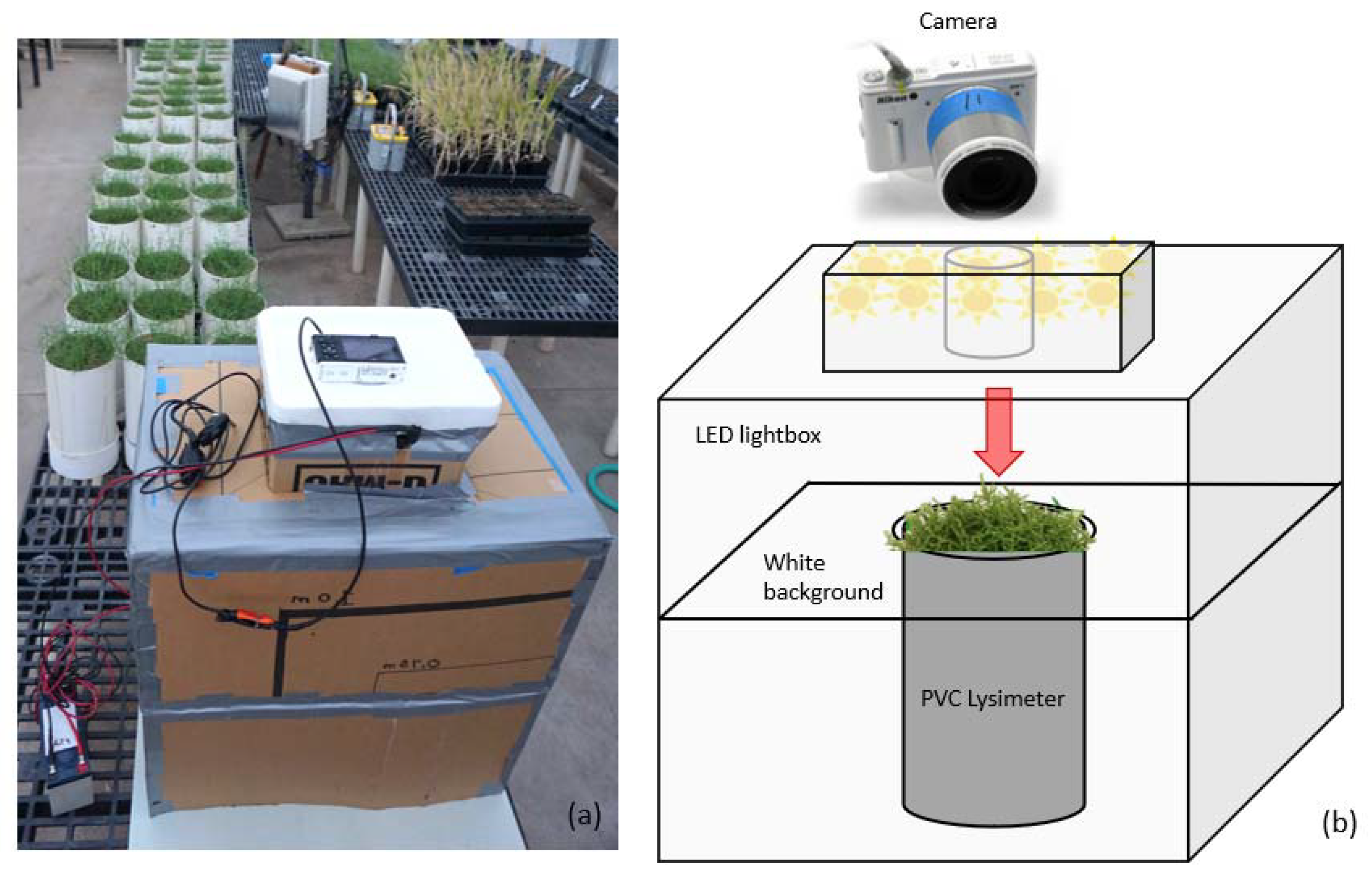
An economical (< $1000) Nikon N1 aw1 DSLR action camera with 11 to 27.5 mm f 3.5 to 5.6 NIKKOR lens and custom-made LED lightbox were used to investigate 72 custom PVC lysimeters (15.2 cm diameter × 30.5 cm depth) growing ‘TifTuf’ bermudagrass (Cynodon dactylon × C. transvaalensis Burt Davy) in two separate greenhouses during the autumn season of 2023, at the U.S. Aird-Land Agricultural Research Center (ALARC) in Maricopa, Arizona, USA. The lysimeters were divided into two runs and treated with four mowing heights (2.5, 5.0, 7.5, and 10.0 cm), three water application levels [(100 × ETa (actual evapotranspiration), 65 × ETa, and 30 × ETa)], and evaluated for visual quality, clipping productivity (biomass), and water use of the 100 × ETa treatment (gravimetric loss). The primary experiment is described in detail in Hejl et al. [102] along with major results. Information regarding the growth setup and environmental measurement are provided in Appendix A. The camera image exposure was controlled by locking manual settings as described below. Image file format, lens distortion, and color correction were tested. The Holland Scientific RapidScan CS-45 product (Holland Scientific, Lincoln, NE, USA), was used, to acquire RED, Red-Edge (RE), and NIR spectral components at 670, 730, and 780 nm wave lengths, respectively. The active reflectance values were collected concatenate with images to provide a camera-independent measurement of the plant's optical signature. Collection of the three spectral bands allowed the calculation of NDVI and NDRE, where both are related, however, NDVI is more common and typical to assess canopy cover but can saturate at higher leaf area index values, while NDRE is considered more sensitive to plant nitrogen and chlorophyll status and incorporates information from the spectral inflection point along the RE region [103,104,105]. Tables of calculated values were managed using MS Excel Version 2401 (Microsoft Corporation Redmond, WA, USA), and statistical analysis was conducted in JMP 15.2.0 (SAS Institute, Cary, NC, USA) software, but a permutation ANOVA technique [106] was implemented in the R programming language (R Core Team 2021) as aovperm from the permuco package.

The custom lightbox design was based on a modification of the well-regarded 2001 approach of Richardson and Karcher [107], and the 2016 Zhang et al. design [108] that incorporates LED lights, each of which employs a portable photographic studio for digital image-based phenotyping of turfgrass. The rudimentary prototype lightbox used in this paper measures 57 (L) × 40 (W) × 74 (H) cm. It was constructed from 0.5 cm thick repurposed cardboard, assembled with tape, and equipped with an internal horizontal image backdrop that fit flush around the 16 cm diameter lysimeter top (182.4 cm2). The camera was positioned with lens protruding into a 24 (L) × 24 (W) × 14 (H) cm upper box containing LEDs. The camera lens was 27 cm distant from the lysimeter and pointed downward from the top of the box through an 11 (L) × 20 (W) × 6 (H) cm polystyrene camera cradle with a 7 cm hole that was 6 cm deep to fit the form of the lens. White printer poster paper was used as a generic, hue-neutral light reflector to cover the inside surfaces of the box. The box was wide enough so that the camera view of the lysimeter top and background would not extend to its sides; therefore, only the lysimeter top and white backdrop were in camera view. For each image sample, the box and one lysimeter were placed on a 60 (L) × 55.5 (W) cm light-colored paper poster board, which was positioned on the greenhouse bench to provide a consistent material foundation.

Photographic illumination was provided by an inexpensive generic 12-volt light emitting diode (LED) strip (Desvorry branded) consisting of 300 individual 6000 K white color lights. The light strip was affixed to the top of the box inside the perimeter around and just above the camera lens. Many LED lights were used for illumination to support light diffusion and reduce of shadows. Change in lighting due to the duration of LED activation was detected, as measured by a pyranometer positioned at the height of the lysimeter top inside the lightbox. The overly inexpensive light source decreased in intensity from 16 to 8 watts m 2 over 360 seconds, described by equation 1:

R a d i a t i o n = 0.00005 \times {S e c o n d s}^{2} - 0.0309 \times S e c o n d s + 16.494

(1)

(coefficient of determination, R² = 0.95), with a steady state of 8 watts m-2 after 360 seconds (standard deviation, STD = 0.537). Therefore, the LEDs were only activated immediately before each lysimeter image sample and then turned off to mitigate fluctuations in brightness. The approach reduced measured illumination variance, resulting in an average of 16 watts m 2 (STD = 0.482) across twelve test runs. Each test run consisted of 7 to 15 seconds of illumination with 60 seconds of de-energized time in between. This scenario was representative of the typical timing for lysimeter data collection of just over one minute per lysimeter.

The camera was set to “manual” acquisition mode with a “manual” exposure, no exposure bias, no flash, and “pattern” focus metering. “Standard color” was selected with no “Active D lighting”. The camera exposure was set to 100 ISO with an aperture of F-Stop 3.5 and a shutter speed of 1/320 second. An 11 mm focal length (equivalent to 29 for a 35 mm crop factor) was used, and the adjustable zoom lens was taped in position. A custom white balance was sampled and recorded on the camera by using the white poster paper placed inside the box and illuminated by the LEDs. The camera viewfinder displayed a circular graphic that was about the same size as the lysimeter top when visualized on the screen. This feature was utilized to verify straightness of camera angle and support geometric consistency between images. The camera display helped verify the time each image was taken and ensured that no settings were accidentally changed between image collections. A custom remote trigger was used to manually activate automatic focus and acquire images. High-resolution 4608 × 3072-pixel JPEG and 4548 × 3012-pixel Nikon NEF (RAW) image file formats were obtained (approximately 5.9 and 12.3 MB in size respectively). This equated to a measurement resolution close to 11 pixels per mm. Three 24-bit sRGB image replicates and one RapidScan composite reflectance measurement were taken consecutively for each lysimeter sample. Average values obtained from the imagery were used for comparison with the individual VQ and NDVI lysimeter point measurements. Lysimeters were imaged approximately every other week for eight weeks. Image processing was conducted on a Dell Latitude 5420 laptop with an i7-1185G7 1.8 GHz CPU and 16 GB of RAM (Dell Technologies Inc., Round Rock, TX, USA) running Microsoft Windows 11 Pro 22H2 64-bit OS (Microsoft Corporation, Redmond, WA, USA). This computer represents a typical consumer-grade product, with the Python 3.12 software (Python Software Foundation, Beaverton, OR, USA) that is commonly used in lower-division academic settings. Jupyter Lab and Notebook software (Project Jupyter, New York, NY, USA) were run using an Anaconda 2.5.0 installation (Anaconda Inc., Austin, TX, USA) and included the Pandas, Numpy, Scipy, OpenCV, PIL, Scikit-Image, Matplotlib, and Seaborn modules. When RAW imagery was used in the Python process, files were initially converted to TIFF (Tagged Image File Format) without compression using Irfan Skiljan’s IrFanView 4.59 (IrFanView, Lower Austria, Austria), which resulted in a file size of 40.1 MB. All imagery was converted to an 8-bit memory depth when processing in Python to reduce computational overhead. An 8-bit image can still display up to 16.7 million colors using 0-255 value tuples. It took approximately 60 seconds to process a single image file on the small laptop computer, regardless of the file type.

Figure 1. The lightbox is shown in greenhouse #1 (panel a, left side) with the camera installed on top. The remote trigger with switch and the 12-volt power supply with 7.5 Ah SLA battery and wires are visible on the left and bottom left side. The lightbox diagram (panel b, right side) illustrates the placement of LED lights and demonstrates how a lysimeter would be inserted into the box and photographed against the white background.

Color correction was performed before application of lens correction using the PerfectColor program from Evan Lund of Evens Oddities (https://www.evenlund.com/). This program was freely available and allowed batch correction of images using the 2014 standard X-Rite Color Checker Classic (24) Legacy panel. It used lookup tables (LUT) generated from a camera profile reference image of the color checker panel that was captured inside the lightbox. Color checker reference values were provided by Babel Color (https://babelcolor.com/), and RawTherapee was used to sample and compare color values using its Lockable Color Picker tool. Image color values were also measured using ImageJ 1.54c for reference and comparison [109]. ImageJ is an open-source Java program credited to Wayne Rasband and contributors, in association with the National Institutes of Health, USA. The software offers powerful image processing and analysis functions.

Lens correction was performed after color correction using Python Discorpy 1.6.0, which can correct radial and perspective distortion by utilizing a grid pattern reference image. Graph paper was photographed inside the lightbox to provide the input pattern. The software calculated polynomial correction coefficients specific to the camera setup. Correction results showed linear grid uniformity of graph paper control images upon manual review. Corrections were batch applied to the experiment sample images. Separately, lens vignette correction was performed in RawTherapee using the settings of 48 strength and 45 radius for JPEG images, and 45 strength and 45 radius for TIFF images.

Color classification areas were determined based on pixel values and a binary mask to segment regions of interest in the original image. The selected classification areas were analyzed as a fraction of the total image area. They represented a manually assessed range for the total living plant material cover, the percentage of yellow senescent or chlorotic plant material, and a generic green color plant material. Details are provided below and in Table 1. The bespoke living plant material cover segment was used to calculate the image discrete color qualities within that area segment. Individual color scalar components were generated across several color spaces. Several basic calculations were conducted to evaluate vegetation indices from existing literature, and custom relationships were also formulated based on linear correlation with NDVI and green cover area. Due to the large number of different calculated terms evaluated (280), only the most relevant metrics that best correlated with VQ and NDVI were selected to report in this paper. Although NDVI was collected at the same time as image metrics, VQ was not. There was an average difference of 2.2 days (STD = 0.92) between the assessment of VQ and the collection of image metrics.

The RGB color space is common in imagery [111], where the R term indicates the intensity of Red, the G term intensity of Green, and the B term intensity of Blue colors. The three terms added together indicate a brightness value. The Hue-Saturation-Value (HSV) color space can be derived from RGB values. It separates the color components into a single angle of Hue (H) ranging from 1 to 360 (or another value range of different graduation). Saturation (S) indicates the linear lightness of the Hue color, and Value (V) indicates the linear brightness. Saturation and Value are typically measured on a scale of 1-100 (or 1 to 255 for 8-bit imagery). A Value of 0 represents black, while a Saturation of 0 indicates gray without any color. Percent living plant cover classification segmentation (%C) was conducted using the HSV color space. Where Hue (on a scale of 1 to 180) ranged from ≥ 27 to ≤ 90, Saturation (on a scale of 0 to 255) ranged from ≥ 60 to ≤ 255, and all brightness Values were included (on a scale of 0 to 255). The generic green fraction (%G) included Hue ≥ 30 and ≤ 60. Green fractional cover was previously reported by Casadesus to support wheat research [112]. Yellow area classification (%Y) involved Hue ≥ 16 to ≤ 26. Both %G and %Y used the same Saturation and brightness Value designations as %C (Table 1).

The Python-based image analysis used in this paper was modeled on the approach exemplified in the TurfAnalyzer (TA) software. TA is a freely available software tool developed by Douglas Karcher in collaboration with Pennington Seed, Inc., and Nexgen Turf Research LLC. [113] based on the progressions of Karcher and Richardson [35,110] who originally used SigmaScan macros to measure turfgrass. It enables analysis of JPEG images for percent green cover and dark green color index (DGCI) and has been used in many experiments [114,115,116,117,118,119,120]. The default color values for TA were included in the Python analysis. These values were determined by converting the full Hue range from 1 to 360 and the Saturation and brightness Value ranges from 1 to 100 in TA to a Hue range of 1 to 180 and Saturation and brightness Value ranges from 0 to 255 for the OpenCV commands, respectively. To better understand the compute process and verify data quality, calculated image values such as mean cover area classifications and DGCI were compared between the two software outputs and found to be equal. However, the more intricate Python approach was selected in this research due to the desire for enhanced process control, the capability to conduct full-resolution computations on TIFF format files, the option to export individual pixel values if wanted, the ability to export additional statistical values for each image, the need for additional calculations involving customized relationships between metrics, and the option to visualize and export individual values, histograms, or index calculations as separate charts.

¹ A comprehensive range of Hue angles was selected for the fraction of living cover area (%C) classification segment, to include lower quality yellow-green living plant material, through the range of green color to higher-quality green living plant material and into any blue-green material (although no blue-green plant material was present). This broad range was chosen to be inclusive of all the living plant material. Selection of the generic green color area (%G) centered around hue angle 45 and was intended to select only healthy vegetation with high chlorophyll and nitrogen contents. The fraction of senesced yellow plant material (%Y) selection included color values below those of the %C, but also excluded the shades of Red and brown colors which indicated soil (the threshold was positioned between the color overlap of brown leaves and brown soil). The three classified color fractions included all brightness Values but used a Saturation threshold of about 24% to ensure that selected pixels contained a color intensity which excluded the white background and bright reflection points. These classification parameters were derived from an iterative process of manual selection and evaluation detailed in the discussion section.

Figure 2. An example lysimeter uncorrected image and three masked views. Experiment treatment 30% water and 5.0 cm mow height is shown in an image taken on 10/26/2023 (Week 2) with associated 0.61 NDVI and 7.0 VQ (panel a, upper left), 97.8% of the lysimeter area covered in live green material (%C) segment (panel b, upper right), resulting in 0.280 DGCI, 0.400 HSVi and 7.010 COMB2 calculation values, with 31.1% yellow (%Y) plant cover (panel c, lower left), and 59.0% green (%G) cover fraction (panel d, lower right).

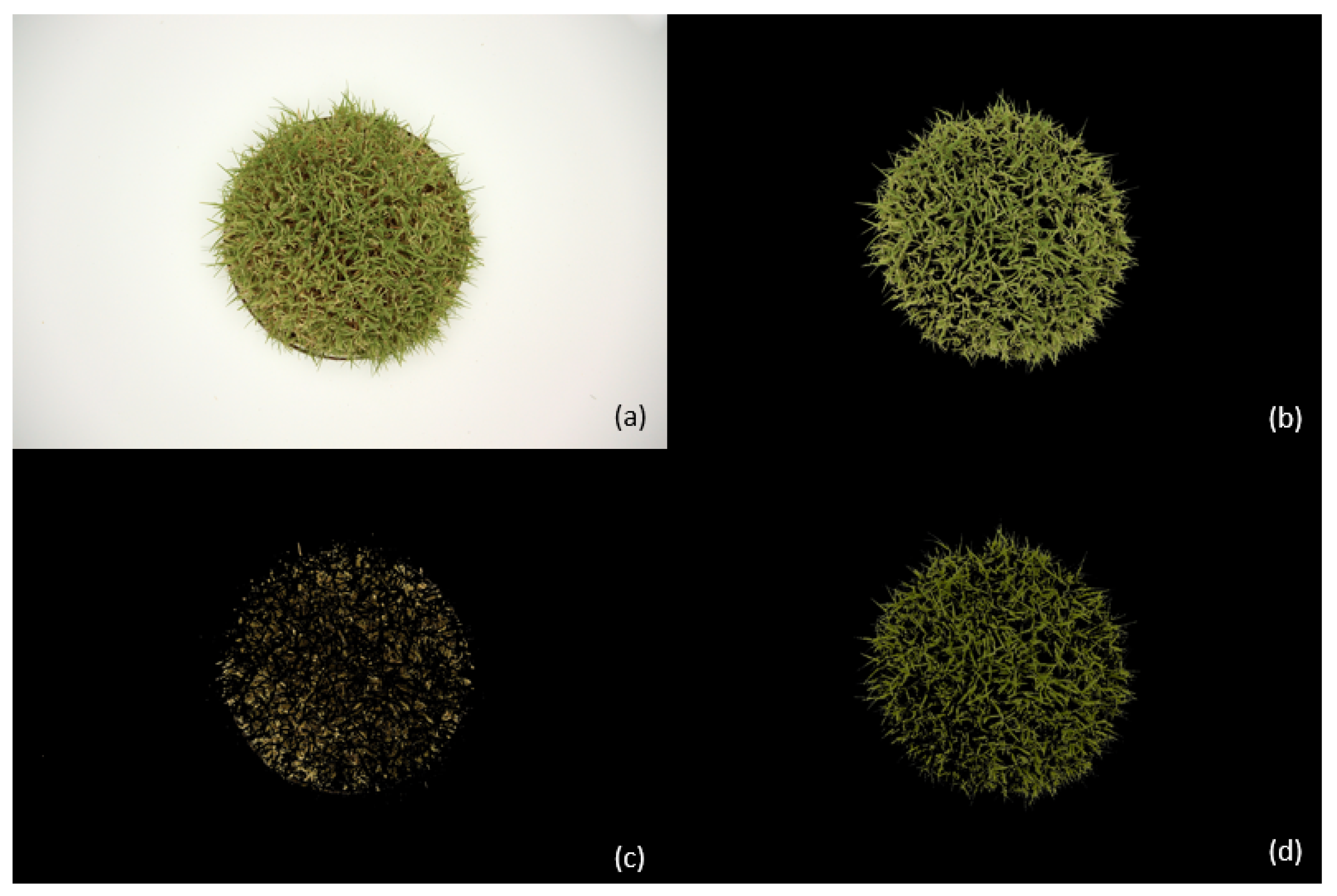
² The upper left (panel a) displays the original 2-D view image sample for a 5 cm mow height and low water treatment. The hue-neutral white background is adjacent to the lysimeter perimeter, with grass leaves extending outward. The lower left (panel b) depicts the HSV-based primary color segmentation of all living plant cover area. This comprehensive range of yellow-green to blue-green %C classification accurately includes all illuminated living plant material and was used as the basis for calculating color qualities in subsequent calculations. The upper right (panel c) shows the %Y fractional area of senescence with plant relevant Hue angles below the %C parameter but above soil. The lower right (panel d) shows the %G cover segmentation of healthy plant material.

This paper evaluated the RGB-based COMB2 calculation from [121], where three vegetation indices were combined for a model intended to be more sensitive to vegetation changes and less affected by soil background. It uses the Excess Green index, which is designed to enhance detection of green vegetation, equation 2:

E x G = 2 \times g - r - b

(2)

from [122], where r, g, and b values are normalized Red, Green, and Blue, the Color Index of Vegetation Extraction index designed to enhance green color for vegetation segmentation, equation 3:

C I V E = 0.441 \times R e d - 0.911 \times G r e e n + 0.385 \times B l u e + 18.78745

(3)

from [123], and the Vegetation Extraction Index designed to emphasize green reflectance, equation 4:

V E G = \frac{g}{(r^{0.667}) \times (b^{\frac{1}{0.667}})}

(4)

from [124], where r, g, and b values are normalized Red, Green, and Blue, and the alpha value of 0.667 was taken from [125] as a generic camera factor. These indices are combined to create equation 5:

C O M B 2 = 0.36 \times E x G + 0.47 \times C I V E + 0.17 \times V E G

(5)

Color spaces beyond the standard RGB and HSV were used. CIE 1976 Lab* (CIELAB) values were calculated with OpenCV, and individual color and brightness scalars were evaluated separately, as well as in relation to each other using various equations. The CIELAB coordinate system was adopted by the International Commission on Illumination (CIE) in 1976 [126] as a color space with increased uniformity relative to human visual perception [127,128]. The CIELAB color space is useful in many applications [129,130,131,132,133] because its colors use the standard observer model for device independency. The CIELAB color space achieves increased human perceptual uniformity because equal Euclidean distances in the color space corresponds to equal perceived color differences. The CIELAB L* term represents lightness, but essentially, the a* term represents a green-to-red color dimension axis, and the b* term represents a blue-to-yellow color dimension axis. This paper uses the color opponent axis ratio of b* to a* (BA), intended to emphasize plant health indications of green and yellow pigment status, and authors are not aware of other phenotyping papers using this ratio although Wanono [134] investigated the ratio of a* to b* to detect leaf nitrogen. A higher BA ratio could signify chlorosis, senescence, or water stress, while a lower value could indicate presence of chlorophyll, nitrogen or increased water use efficiency.

An additional image-based equation was created to compare with standard DGCI. The unconventional Hue difference illumination ratio, or HSVi, equation 6:

H S V i = H - (\frac{S}{V}) \times 40^{- 1} - 0.3

(6)

This equation utilizes the HSV color space, where the simple ratio of Saturation and Value was subtracted from Hue, and the result was shifted and offset to scale roughly into a range of 0 to 1. By considering the saturation-to-value ratio we capture a relative color intensity, and so as brightness increases the saturation impact reduces. A higher ratio indicates more vivid color relative to brightness. This nuanced HSVi approach modulates Hue angle as a function of color purity and attenuates the positive effect of Hue using lighting to discriminate minor plant features. Therefore, context is important for interpretation, because a larger HSVi result may indicate healthy but less dense vegetation with higher reflectance, while lower values may indicate stressed or the presence of very dark green vegetation.

Calculated metrics were summarized in tables and related to the experimental class structure. To test the effects of experimental treatments, response variables were assessed using a robust permutational multivariate analysis of variance (permANOVA). Non-parametric permutation ANOVA models are useful in environmental analysis to better handle complex data [135,136,137]. Neither the VQ nor the NDVI data in this paper use camera technology. Therefore, VQ data reported previously and NDVI measurements were chosen as independent references to compare with the image-based data [36,138,139]. The authors are unaware of other published works detailing the sensitivity of file format and image corrections (JPEG, TIFF, LC, and CC) on phenotypic image calculations for plant phenotyping.

Image-based metrics were calculated and compared with reference measurements to test the effects of a file format with standard JPEG compression (JPG), NEF (RAW) to lossless TIFF conversion (TIF), and image adjustments for geometric lens correction (LC), and color correction (CC). Pearson’s correlation coefficient (R) and coefficient of determination (R²) values were calculated, and the image metrics that best corresponded to each reference measurement were selected for reporting. A sensitivity analysis of calculated metrics was conducted to assess the impact of file format and image corrections. Significant differences were tested and a comparison of treatment effects on image metrics, VQ, and NDVI was performed using non-parametric Kruskal-Wallis median test and Dunn’s ranked test with JPEG as control. In a similar approach, the coefficient of variation was evaluated to investigate the effects of file format and image correction on replicate images. An NDVI time series overview for the original experiment is presented for the first time in this paper, and time series data for two image-based color metrics are offered to show comparative differences in behavior over the course of the experiment.

3. Results

The %Y quantifies a pixel-based segment of percent cover across the lysimeter top area for yellow-colored senescent plant material (Table 2). Lower values of yellow can indicate higher quality turfgrass. The %G area pixel-based fraction indicates the portion of healthy green plant material. DGCI describes the color of turfgrass, where higher values indicate a darker green turfgrass [140]. The HSVi calculation is akin to DGCI as it also describes plant color. HSVi is nuanced, where higher values can indicate a higher quality of green for turfgrass, but context is important for interpretation. The BA ratio of the b* and a* color scalars also represents a nuanced relationship where higher values indicate more yellowness relative to redness and lower values indicate more blueness relative to greenness.

3.1. Linear Correlation between Variables

Linear correlation and percent variance explanation of the image calculations was analyzed. This involved the continuous variables Visual Quality (VQ), grass clipping production (mg d^-1), water use (mm d^-1), NDVI, NDRE, NIR, RED, and RE (Table 2). Results show that %Y cover area correlated most strongly with VQ, the calculation of DGCI correlated strongest with mg, COMB2 correlated most strongly with mm, %G correlated strongest with NDVI as well as RED, BA correlated most strongly with NDRE, and RE, and HSVi correlated strongest with NIR. However, there was no clear trend in correlations regarding the effects of the image corrections or file format.

² Data suggests that selected image-based calculations correlate with VQ, clipping production (mg d^-1), water use (mm d^-1), and spectral reflectance values. However, the image format and correction process only sometimes improved resultant correlations. The uncorrected TIF and JPG LC for %G classification area exhibited the strongest correlation with NDVI and RED respectively, but there was a nominal 0.000 and 0.001 respective difference in R² between the uncorrected TIF and JPG LC with JPG for each. The relationship between BA with NDRE, and RE showed strongest correlation, but R² only improved by 0.004 for NDRE and 0.003 for RE over the uncorrected JPG. %Y and VQ was similar, where the JPG LC CC showed the strongest correlation, but the R² was only 0.005 higher than the uncorrected JPG. DGCI TIF CC correlated best with productivity, but the correction showed only minor differences in R² with a 0.098 increase. Likewise, the HSVi TIF CC correlated strongest with the NIR but the R² only increased 0.014. One metric, COMB2, exampled a big improvement with TIF LC CC. The COMB2 had the strongest correlation with water use where it exhibited an R² value 0.310 higher than its uncorrected JPG counterpart. Therefore, it would be improbable to apply none, all, or any individual correction procedure and consistently achieve the highest correlation results across this variety of image-based calculations.

3.2. Effects of Image Corrections on Calculated Metrics

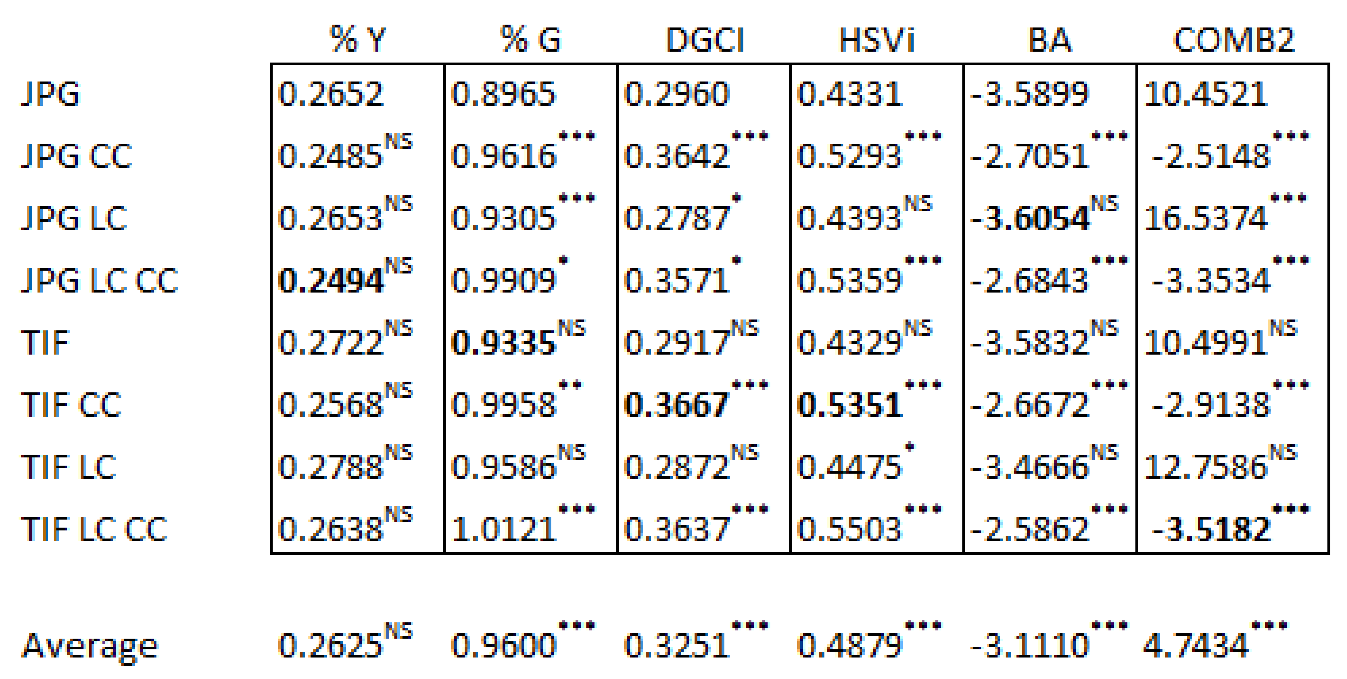
³ The TIFF file format and three correction types were compared against the uncorrected JPEG format to assess their impact on median values for six image-based metrics. Results are mixed regarding the significant effects and the magnitude of the correlations with reference measurements. There was a significant difference among all the median values of calculated metrics, except for %Y, even though the JPG LC CC shifted the median value of %Y by 1.6%. TIF format without correction shifted the %G median by 3.7%, but it was not significant. Similarly, JPG LC shifted the BA median by 0.906, but it was not significant. However, TIF LC did significantly shift medians for DGCI and HSVi, by 0.075 and 0.102 respectively. Most striking was the effect of corrections on COMB2, where TIF LC CC significantly shifted the median by -13.97 (or 133.7%). Corrections for four of the six metrics that resulted in the highest or lowest median values did not correlate strongest with their associated reference measurements; however, DGCI TIF CC resulted in the highest median value, and it correlated most with productivity (Table 2), while COMB2 TIF LC CC resulted in the lowest median value, and it correlated strongest with water use (Table 2). Median values did tend to improve along their relative scales with CC. However, there was no clear trend across all the metrics. Therefore, this data supports the idea that neither the file format nor any specific image correction consistently improved model power for these image-based calculated metrics.

Table 3. Medians and significant difference for file format and correction effects utilizing a one-way Chi-square approximation of the non-parametric Kruskal-Wallis test, and Dunn’s joint ranks test with Bonferroni adjustment using the JPEG file format as control. Bold font indicates the correction for each metric variable which correlated best with its associated reference measurement (Table 2). Significant difference in median values is noted as, not significant, p ≤ 0.05, p ≤ 0.01, and p ≤ 0.001, by symbols, NS, *, **, and *** respectively.

3.3. Detection of Experiment Treatment Effects

⁴ A robust non-parametric permutation-based ANOVA was chosen to handle the skewed and complex environmental variables. Results indicate the effect size and likelihood of significant treatment effects on image metrics and reference measurements. Mowing height had a significant impact on all variables and was primarily explained by VQ. The irrigation effect was significant for all variables and was also primarily explained by VQ. All variables were significantly affected by Date, where the HSVi and DGCI prominently explained the Date effect, followed by BA. A substantial portion of the overall effect size for NDVI, %G, and %Y was also attributed to the Date, indicating detection of the autumn seasonal trend towards biological dormancy. The interaction between mowing height and water was significant for all variables except DGCI, and was best explained by COMB2, although this interaction category had the most unexplained variance overall. The interaction effect of mowing height by date was significant for all variables except VQ and DGCI, and was best explained by COMB2 with a medium effect size. The irrigation-by-date interaction was significant for all variables except DGCI and HSVi, where VQ provided the best explanation followed by %Y. The three-way interaction effect was significant for all variables except VQ and %G, but was explained most by COMB2, indicating the most sensitivity to experimental treatment interactions with this combination index variable.

These results suggest that the different metrics play distinct roles in resolving various aspects of the biological information signal. The mean values were significantly different for all treatment effects, suggesting potential utility for detecting variations in irrigation quantity, mowing height, changes over time, and their interactions. The COMB2 variable may have outperformed NDVI with higher categorical effects significance, but the ηp2 and F-values were highest for %Y. The low effect sizes for the interaction of mowing height and irrigation suggest that the dynamics of this treatment merit further investigation. Additional tables of the p-values and F-values used to create Table 4 are provided (Appendix A) to offer more precise probability values of significant differences and additional model fit measures.

3.4. Image Corrections Effect on Replicates

⁵ Three replicate images were initially taken in rapid succession for each of the 316 lysimeter samples. A coefficient of variation (CV) was calculated for each image metric and with each image correction, and the CV values were averaged across all collections for each file type and correction. The average values of CV were compared to the correlations (Table 2) and ANOVA (Table 3) results.

Significant differences in image correction effects were observed in the average CV values between replicated images for all metrics except %Y and BA using the Kruskal-Wallis test of medians and Dunn’s test with JPG as control. The JPG LC CC for the %Y correlated best with VQ (Table 2), even though TIF LC CC had the lowest CV. The %G TIF data correlated best with NDVI and RED reflectance (Table 2), even though TIF LC CC lowest CV and a noticeable difference for CC with reduced CV was evident. The DGCI TIF CC best correlated with productivity (Table 2), even though the uncorrected JPG and TIF formats showed lower CV values and there was an increased CV with LC visible. HSVi calculation in TIF CC imagery correlated best with NIR reflectance (Table 2), even though the TIF and JPG had lower CV values and a general increase in CV with CC was visible. The JPG LC BA calculation best correlated with NDRE and RE reflectance (Table 2), even though the uncorrected JPG had the lowest CV. The COMB2 calculation of JPG LC imagery correlated best with water use, even though the uncorrected TIF had the lowest CV and there was generally a higher CV with corrections.

Table 5. Coefficient of variation (CV) for replicate images are compared across file format and image corrections. The median CV values for selected calculated metrics across each image correction are tested for significant difference using a one-way Chi-square approximation of the non-parametric Kruskal-Wallis test of medians, and Dunn’s joint ranks test with Bonferroni adjustment and the JPEG file format as control. Bold values note the image correction that resulted in the highest correlation between the image-based calculation variable and its associated reference (Table 2). Significant difference in median value is noted as, not significant, p ≤ 0.05, p ≤ 0.01, and p ≤ 0.001, by symbols, NS, *, **, and *** respectively.

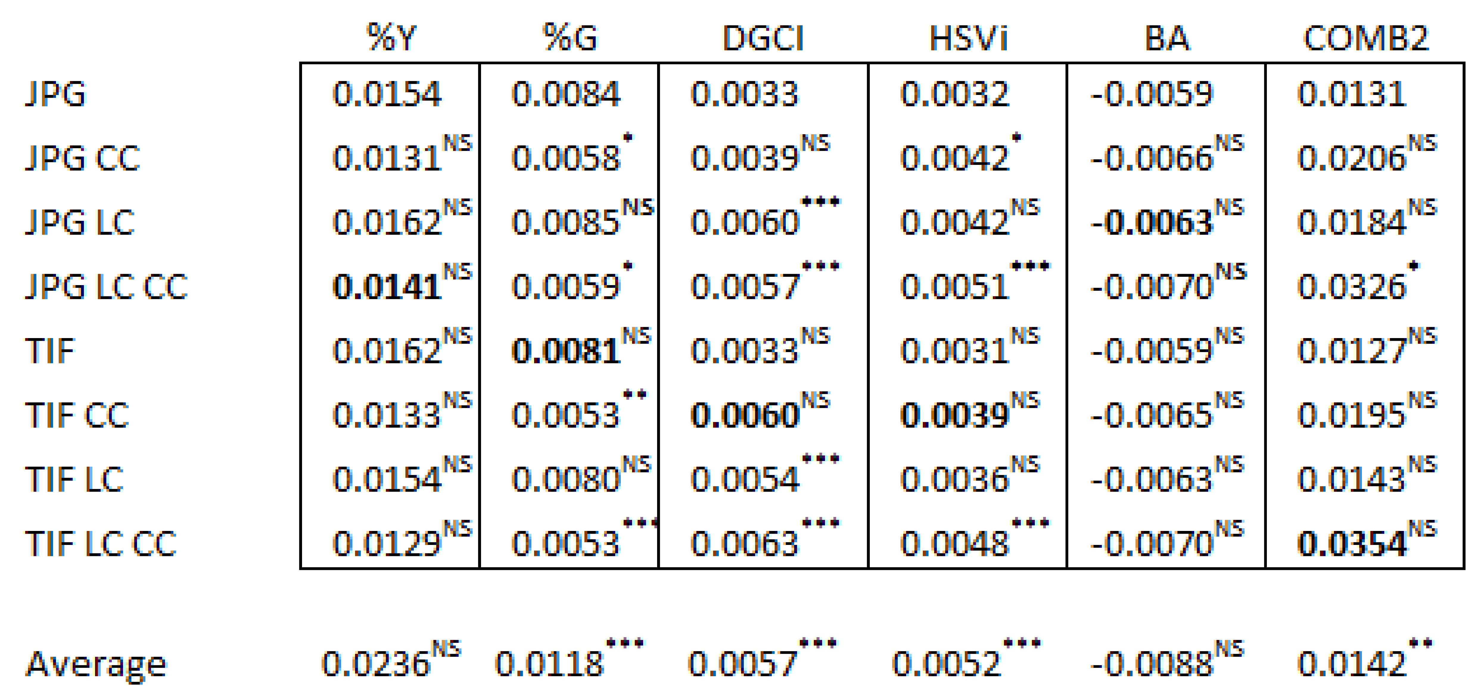
Image corrections significantly affected the median CV of image replicates in four out of the six metrics. However, the median CV of the image replicates for each calculated metric did not explain the subsequent model fit. Higher values of CV did not result in reduced explanatory capacity. Yet the uncorrected JPEG file format showed a CV lower than the overall average for each metric. These results demonstrate a weak relationship between the dispersion in replicates and subsequent correlation with reference measurements. Therefore, the median dispersion of image values from replicates did not indicate a better model fit or better explain the reference measurements for these six calculated metrics. The analysis of CV also did not consistently identify a specific image format or correction method that led to higher or lower data dispersion. This result supports the notion that the effects of the image corrections applied are present, but they are difficult to parameterize and explain across multiple and varied image-based calculations.

3.5. Time Series Charts for Three Metrics, NDVI, %Y, and COMB2

³ NDVI was not previously reported by Hejl [102] and is shown here (Figure 3) to illustrate the utility of this common measurement, which was used as a reference for evaluating the imagery data in this paper. Treatments are displayed in a time series throughout the autumn season experiment. A general downward trend in NDVI was evident, but several treatments exhibited increased NDVI over the first third of the experiment before decreasing thereafter. At the beginning of the experiment, the shorter mowing heights automatically had a decreased presence of green biomass, resulting in lower NDVI values compared to taller heights. As the experiment progressed and the irrigation deficit treatment intensified, shorter mowing heights were able to sustain their green biomass presence longer. In the lowest irrigation treatment, the relative NDVI values ranged from largest to smallest, corresponding to the heights from shortest to tallest. The middle irrigation treatment also exhibited this effect, but with less pronouncement, where NDVI values became comparable by the end of the experiment. The full irrigation treatment exhibited the highest NDVI values overall, and taller mowing heights were more effective in preserving green biomass when given adaquate water. The NDVI values for the fully irrigated plants were generally arranged from taller to shorter heights, except for the shortest height, which had the second highest NDVI values and was comparable to the tallest full irrigation treatment. Results suggest that green biomass presence may be prolonged under reduced water availability with shorter mowing heights. Additionally, a moderate reduction in water availability may have a limited effect on NDVI regardless of mowing height. However, the largest green biomass as measured by NDVI can be expected with higher mowing heights and full demand replacement water applications.

⁴ VQ was previously reported by Hejl in 2024 [102]. Therefore, a time series of the senesced plant indication %Y area segment is shown as a proxy, by experimental treatments as calculated from the JPG LC CC image set (Figure 4). This proxy had the highest correlation with VQ, an R² of 0.79 (Table 2) and demonstrated the highest effects size (Table 4). The %Y was scaled as a percentage of the top inside area of the lysimeter. Values could exceed 100% if yellow-colored leaves covered the lysimeter area and extended beyond the perimeter of the lysimeter top. The classification of the %Y showed a more consistent trend than the NDVI, basically increasing for all treatments across the experimental period. However, shorter mow heights generally resulted in less yellow presence. Unexpectedly, the 7.5 cm mow height showed more %Y than the 10 cm height for both the highest and middle irrigation levels indicating a possible microclimate, root system, or nutrient allocation impact. Results suggest that image-based classification of the fractional yellow area can be an effective metric for assessing visual quality in turfgrass. It can also differentiate mow height effect when water is significantly reduced.

⁵ COMB2 data is presented in time series to show the different behavior of this color metric over time, as compared to NDVI and %Y, because it most correlated with water use (Table 2), and because it showed significant difference for all experimental effects (Table 4). A complex and nuanced response is evident using this combination of vegetation indices. Higher COMB2 values suggest healthier vegetation and more biomass. This can be seen in first half of the experiment where values decline as plants tended to decrease in quality over the experiment. However, these results are difficult to interpret because unlike NDVI and %Y (Figure 3 and Figure 4), there are larger COMB2 initial treatment differences that converge as the experiment progressed perhaps indicating the effects of season, and the lowest irrigation with the two taller mow heights increased over the experiment, even though their color quality decreased perhaps indicating change in canopy density. The initial separation regarding mow height groupings evident across the irrigation levels may suggest distinct canopy structures. Another consideration is that the image correction effect was very large for this metric (Table 3), where different corrections changed the correlations with different reference measurements (Table 2). Nevertheless, statistical significance with treatment effects results suggests an information contribution from the COMB2 color term with TIF LC CC application, therefore further study is warranted.

Additional time series charts for the metrics of %C, %Green, DGCI, HSVi, NDRE, NIR, RED and RE metrics are provided in the supplimental.

4. Discussion

To assist researchers, students, and managers, the authors propose a practical approach that includes accessible camera controls for collecting relevant image-based plant phenotyping data. Locked manual photographic exposure settings that balance a lower ISO, moderately higher F-Stop, and lastly a higher shutter speed should be selected based on the camera’s response to the overall lighting intensity of the target environment. Next, it is important to measure and set a customized white balance for the specific spectral intensity of the ambient illumination, rather than relying on a pre-set color temperature. Consider that a RAW file format allows post-processing of the total camera-generated data. Yet a lossless TIFF file format will retain all the image pixel color values. On the other hand, while the JPEG format is lossy, high-resolution imagery could mitigate the effects of compression loss and may therefore be acceptable for plant phenotyping functions. Although image data corrections are important to consider [141], they can be challenging to implement, and their effects could be difficult to quantify and report. Therefore, it may be acceptable to rely solely on modern camera technology with simple exposure controls and achieve sufficient image data quality to perform basic plant phenotyping for advancement of scientific knowledge. However, in some instances, such as with the calculation of COMB2 in this paper, image corrections induced significant effects strong enough to change result interpretations. To overcome possible gaps in knowledge, transparent standardized protocols and detailed metadata is needed that includes cross or independent validations, and robust statistical analysis utilizing sample replicates or controls.

Utilizing a simple camera-based plant phenotyping approach, the highest R² values were observed in the relationship between VQ with %Y area classification, and NDVI with %G area classification (Table 2). Traditionally, the evaluation of turfgrass has focused only on green color areas. However, our findings reveal that presence of yellow, which demonstrated congruence with human perception of quality and significant treatment effects, offers insight to assess the relative presence of green biomass in turfgrass. Casadesus [142] introduced a “Green” and “Greener” segmentation in wheat, incorporating some yellow into the “Green” classification. By introducing a dedicated yellow cover class, such as the %Y metric employed in our study, the yellow stems and senesced plant material is captured and quantified more comprehensively. A more complete classification system that includes the readily observable visual cue of yellow may allow for greater precision in evaluating the composition and health of turfgrass which could improve phenotyping analyses.

Further research is warranted to clarify the COMB2 term in relation to plant biological status because the detected treatment effects significance with image corrections (Table 4) suggests a utility of this color calculation to support understanding of plant phenotypic traits, but COMB2 behaved differently than traditional terms like NDVI (Figure 5 and Figure 3). Although the COMB2 calculation may provide some phenotypic detection capability, it does not predict water use. Similarly, although DGCI correlated strongest with mg clipping production (Table 2), the relationship was not robust enough to explain most of the variation in reference measurements. The BA ratio correlated most with NDRE and RE reflectance, while the novel term HSVi correlated most with the NIR spectral reflectance component (Table 2). Therefore, calculation of BA or HSVi may be useful to roughly estimate respective RE or NIR spectral reflectance when only color camera data is available. The BA ratio may serve to emphasize yellowness relative to redness and provide an indication of chlorophyll content or plant health, but authors did not find reference to this ratio in plant phenotyping literature so additional research is warranted. HSVi showed stronger correlation with NDVI than DGCI (Table 2). Therefore, variations in this illumination modulated Hue angle determined by HSVi may help detect pigmentation status or tissue health across the biomass area or over time. However, because authors are not aware of other research using the HSVi image calculation for plant phenotyping, additional research is needed to determine biological significance.

This paper demonstrates how image acquisition using consumer cameras with simple controls enables not only standard calculations of traditional metrics like the green area or DGCI, but also facilitates additional calculations like bespoke yellow area, HSVi or BA which may be valuable in the description of plant phenotypes. Although it could be possible to avoid image corrections and still achieve acceptable results when simple exposure controls are used, the application of appropriate image corrections before calculation of image metrics will likely generate the most useful information. However, the varied and mixed correction effects results in this paper suggest further research is necessary to precisely identify the best methods to maximize corrections utility in image-based plant phenotyping.

Though the simple image-based approach in this paper used to identify basic cover and color features was successful, limitations persist, and several improvements can be made. First, to enhance color accuracy and consistency in subsequent investigations, the illumination source will be upgraded to a professional-grade LED option with a high color rendering index [143,144], such as exemplified in the Waveform Lighting Absolute Series ^TM product line. Second, considering that the camera selected was released in 2013, a more modern camera may incorporate improved technology and increase the quality of the base data. Third, although no errors were detected, adjusting the camera lens aperture 3.5 F-Stop to a higher setting of around f/8 to f/11 would elongate focal depth of field, decrease lens vignette artifacts, optimize lens sharpness, and reduce chromatic aberration without inducing major diffraction. Fourth, improved computational pipelines capable of handling RAW-based imagery [145] are anticipated to become more widely available and easier to use in the future. While uncompressed TIFF format imagery was processed in the Python pipeline used in this study, larger files are more challenging to manage, and there is less software support for uncompressed file formats compared to the common JPEG form. Yet handling all the image information generated by the camera exposure is expected to improve data quality. Likewise, advancements in color correction [146,147,148] software are expected to become more accessible over time. The authors plan to obtain a license and use the Adobe Lightroom commercial software (and they may use the Python color-checker-detection library) to make color corrections in future experiments. A more robust color correction procedure could enhance data quality. Given the high image resolution capabilities of modern cameras, JEPG compression of high-resolution imagery may be acceptable for proximal measurement [149,150,151,152]. Although camera and lighting limitations are expected to introduce some level of error [153], a careful assessment is necessary to determine whether inherent camera-induced representational errors are acceptable. The value of corrections should be weighed against their implementation costs and the potential introduction of new error sources. Refinement of the corrections methodology is essential. This study used a sensitivity approach to compare the effects of eight individual image types on six image metric correlations with eight reference measurements, including VQ and NDVI. The study indicates that %Y, BA, and HSVi have the potential to differentiate the effects of experimental treatments in addition to the more traditional %G and COMB2. However, it also highlights challenges in quantifying the effects of image corrections across diverse metrics.

The effectiveness of color corrections and other image adjustments to enhance data quality for a specific plant phenotyping collection is ambiguous. While corrections are sometimes made, evidence of improvement may be lacking [154,155]. There are well-developed theoretical best practices for corrections [156,157,158,159,160,161], but additional guidance could be provided to quantify the effects of image data adjustments under various real-world conditions. This would help understanding and determination of which imagery correction procedures are necessary in a particular circumstance. For instance, Chopin demonstrated that their camera profile for proximal field imagery was better fitted using a least squares quadratic transformation rather than linear [162]. Despite the challenges posed by a diverse range of camera products, application spaces, and vegetative variability, clear standards for operations specific to various applications would be of benefit to users. The provision of clearer guidelines and empirical evidence to describe the effects of image adjustments would allow practitioners to make more informed decisions, ultimately enhancing the quality and reliability of plant phenotyping data.

The findings in this paper show that the image corrections applied resulted in inconsistent outcomes. While correlations with reference measurements generally improved with image corrections, improvements were often minor and sometimes negative. Only %Y showed no significant effect from the TIFF file format or the image corrections, while CC did cause large significant differences in COMB2, BA, DGCI and HSVi (Table 3). The mean coefficient of variation for replicates was significantly affected by corrections for %G, DGCI, HSVi and COMB2 (Table 5). The optimal combination of file format and image corrections improved R² values for five out of the six image metrics but resulted in less than 2% improvement. However, COMB2 was improved by 31% (Table 2). This suggests that the application of all standard image corrections may not automatically improve plant phenotyping results, and yet lack of best file format and correction implementation could lead to oversight of crucial relationships. An improved statistical evaluation using a larger and more diverse set of images and reference measurements, including the observation of additional plants beyond TifTuf over a longer period is needed to gain deeper understanding of the image adjustments effects and inform best practices. Furthermore, the inclusion of more robust phenotyping equipment to provide thermal, hyperspectral, florescence and structural information would better contextualize the potential of the traditional camera.

Dynamic selection is an easy way to determine and verify color-based cover classification areas. These areas can be parametrically refined using gradient-based selection masks, included in TurfAnalyzer software and common in commercial image editing applications like Adobe Photoshop. By manipulating the criterion control, users can update a selection on the display of an evaluation image and visually assess whether the proper regions of interest are captured. This dynamic process enables users to determine if a particular image metric is responding to an intended color or feature while ensuring that unwanted colors and features are excluded. A similar computational process can be developed with Python scripts and was used for this paper. Given the variability in illumination conditions and camera-specific factors such as sensor characteristics and color processing algorithms, it is recommended to perform iterative visual assessment and adjustment of segmentation parameters to ensure accurate identification and selection of target chromatic values in the image data. This process certifies that correct regions are selected based on the predefined parameter set. Related, the export of a validation image, which consists of the intersection between the original image pixels and the selection mask (including its inversion) enables a zoomed-in view for more detailed inspection of feature transition edges. Detailed scrutiny, perhaps to the limit of the pixel resolution, can reveal whether the target feature area has been fully segmented by the classification parameters employed. TurfAnalyzer software outputs image files that display mask intersection results. However, these images are of reduced resolution and do not depict the original pixels themselves. The Python approach used in this paper enabled the extraction of full-resolution pixel selections output to individual image files that could be closely evaluated.

As part of the exploration process, consideration was given to the Python-based plant phenotyping research software PlantCV (https://plantcv.danforthcenter.org/). Despite its provisions for color correction and many analysis functions, its design did not align with the generic approach of this investigation. Traditional PlantCV operation requires a specific color correction panel to be present in each image, which can pose a geometric obstacle inside a compact lightbox. Although having a dedicated correction reference panel in each image provides for superior batch correction compared to using only one reference image for an entire set, the production and processing of dedicated correction panel views increases complexity, reduces the usable image analysis view space, and may not overcome errors due to inconsistent illumination across a single image. Professional software, such as Adobe Photoshop and Lightroom, are often used to color-correct imagery [163,164,165,166]. However, these tools were not utilized in this study absent their commercial license. Therefore, although color correction is advantageous for comparing imagery taken at different times, in different illumination scenarios, and from different cameras, the benefit of color correction must be weighed against the additional complexity it introduces. Moreover, there is a possibility that color correction can introduce errors that may be difficult to quantify. Thus, the decision to implement color correction should be made judiciously, considering its potential positive impact and the trade-offs involved.

Achieving geometric regularity in images through lens distortion correction is a common enhancement, but it may be challenging to implement. An improved lens correction process could aid higher-quality data results in plant phenotyping [167]. Although the Lensfun database of lens artifacts was available for the Nikon lens used, authors found the correction to be insufficient even after a second manual adjustment was included. This may be due to minor manufacturing imperfections unique to the specific lens used. While RawTherapee (Creative Commons 4.0), GIMP (Crunchbase Company, Charlotte, NC, USA), and Pablo d’ Angelo’s Hugin software (https://hugin.sourceforge.io/) were employed for lens correction, the Python Discorpy package emerged as the most effective solution, offering well-documented tutorials. However, further refinements may still be possible. For example, nominal changes were observed for Hue angles (0.002%) between JPG and JPG LC, while more substantial alterations occurred for Saturation (decreased by 3.8%) and Value (increased by 11.6%). This equated to an increase in RGB (Red by 12.2%, Green by 11.6%, and Blue by 14.7%), therefore LC brightened as well as geometrically corrected images. Consequently, the accuracy of the corrections, a potential new source of error, the added challenge in making corrections for each camera setup, and a subsequent benefit from LC must be balanced together. A straightforward LC result verification is needed to better understand the extent to which LC may improve or degrade a particular imagery set. Separately, the related lens vignette was easy to correct using the RawTherapee software. The resultant brightness gradient from image edge to lysimeter edge across the white background could be sampled to verify basic brightness uniformity. Noting that the artifact effect was negligible for our dataset, other phenotyping images may require additional steps to account for vignetting. Despite challenges, image corrections are expected to improve the accuracy and reliability of resultant data. This calls for continued exploration and refinement of correction methodologies across the diverse imaging setups used in plant phenotyping.

Although a lightbox with many LEDs can provide consistent illumination to facilitate the capture of extensive gridded optical data [168,169,170], its usage imposes major limitations on sample throughput. Inserting each individual lysimeter into the lightbox for imaging was considerably slower (approximately 60 seconds) than the VQ assessment (approximately 3 seconds) or NDVI measurement (approximately 15 seconds). Although a robotic high-throughput plant phenotyping greenhouse can address this restriction [171,172,173,174,175,176], its adoption comes at substantial monetary and complexity cost, albeit more generic versions are being developed [177]. Some experiments have imaged multiple greenhouse plants outside the lightbox omitting robotics [154], but the ambient illumination is likely more varied across each image. Even when a color correction panel is present within each image collected, inconsistent lighting across the entire image can compromise the accuracy of color correction. Hence, improved methods may entail consistent illumination [178] and enable plants to be imaged without the need for relocation.

Optical cameras only measure in the RGB color spectrum (approximately 420 to 700 nm). Beyond this range lies spectral information that is significant for researchers but surpasses the detection capacity of standard cameras. Consequently, the optical camera alone cannot detect the complete spectral reflection of vegetation. Another limitation of the camera sensor is the 2-D representation it generates. Although photogrammetric or structure-from-motion techniques can be used to amalgamate multiple images into 3-D point clouds, incorporating a second view perpendicular to the nadir would provide more plant information and allow for a basic 2.5-D model with just two images, and reduced compute requirement.

Incorporating an up-looking optical diffuser with filters that transmit the RGB frequencies of the camera detector, similar to the design of some UAS multi-spectral cameras [179] like the MicaSense Altum or RedEdge cameras (AgEagle Aerial Systems Inc., Wichita, KS, USA), which are designed specific to their spectral sensitivities, would enable a solar cosine correction [180] frame by frame onboard the camera. This may diminish the value of color correction post-processing and greatly expedite the information process while increasing data quality.

The NDVI measurement used in this paper was derived from a unique active optical sensor technology. Unlike passive sensors, this technology allows measurements in various lighting conditions. Although the instrument used provides a set of raw values and basic statistics from its high-frequency sampling, it only offers a single data point per measurement. An NDVI camera would provide additional spatial information through its pixel grid; however, considerations related to ambient light would come into play. The authors are unaware of any active NDVI camera product.

Micrometeorological measurements of the growing environment are important in plant phenotyping. At a minimum, measurement of photosynthetic radiation, along with sensible and latent heat, provides a context for plant growth (Appendix A). Even minor discrepancies between the expected environmental values, such as air temperature, and the actual values measured at the precise location of the plants, can accumulate over a growing season and impact results. There can also be short-duration events, such as loss of greenhouse controls or abrupt outside weather changes, which can affect plant growth inside a greenhouse. These events may go unnoticed without continuous environmental measurements at sufficient temporal resolution. In this study, greenhouse environments were measured at a frequency of 1Hz, ensuring a comprehensive characterization of the growing conditions. However, the plant images were only captured every two weeks. Increasing the frequency of image capture would facilitate the association of temporal growth indicators present in the imagery data with the measured environment. This would lead to a more comprehensive understanding of environmental effects on observed biological results.

5. Conclusions

A consumer-grade camera and custom-fit lightbox made from rudimentary materials were used to explore a cost-effective method for plant phenotyping. Image-based metrics were calculated using open-source software on a laptop computer and enabled the comparison of human-assessed VQ and active NDVI measurements with image data to determine phenotyping utility. Statistical analysis revealed the highest R² values for VQ and NDVI with the image-based calculations of %Y and %G areas respectively. A novel HSV color space calculation, termed HSVi demonstrated the highest R² with NIR, while the CIELAB b* to a* ratio correlated best with NDRE and RE reflectance. Even though DGCI exhibited the highest R² value for biomass productivity, it did not explain most of the variation. The COMB2 calculation showed significant experimental treatment effects, superior to VQ and comparable to NDVI but was difficult to interpret. COMB2 correlated strongest with water consumption but was not adequate to serve as a proxy. %Y displayed improved overall treatment explanatory power for the experimental effects. Guidance on photographic exposure control was provided to improve the quality of image-based phenotyping data, along with a discussion on software options, processes and limitations. This study indicates that modern camera technology is robust enough to empower plant phenotyping for research and commercial applications that involve cover and color quantification. However, the imagery did not fully describe water use or clipping productivity. Despite testing color and lens corrections and the use of uncompressed image format, no large and consistent improvement in the image-based calculations were observed. This suggests that lossless format and corrections may not always be necessary for standard plant phenotyping when modern cameras, sufficient illumination, and straightforward exposure controls are utilized. A method to quantify the effects of image corrections relative to plant phenotype is needed to determine appropriateness for resolving plant traits of interest with sufficient precision. Parameterizing the influence of corrections on image-based calculations for different phenotyping metrics would strengthen the connection between photographic digital information and plant biological processes, standardizing and enhancing phenotyping practices.

Supplementary Materials

The following supporting information can be downloaded at the website of this paper posted on Preprints.org, Figure S1: F-values and p-values for experimental effects ANOVA (Table 4), additional individual time series charts of %C, %G, DGCI, HSVi, NDRE, NIR, RED and RE metrics.

Author Contributions

Conceptualization, M.C. and R.H; methodology, M.C. and R.H.; software, M.C.; validation, M.C.; investigation, M.C. and R.H.; resources, R.H. and C.W.; data curation, M.C.; writing original draft preparation, M.C.; writing-review and editing, R.H. and D.S.; visualization, M.C.; supervision, R.H.; project administration, R.H. and C.W.; funding acquisition, R.H. and C.W. All authors have read and agreed to the published version of the manuscript.

Funding

Please add: This work funded by the United States Department of Agriculture, Agricultural Research Service, as part of National Program #215, Research Project #438136, CRIS 2020-13210-001-000D.

Institutional Review Board Statement

Not applicable.

Informed Consent Statement

Not applicable.

Data Availability Statement

Datasets and imagery are available upon request.

Acknowledgments

Julia Stiles for process quality control, John Heun for engineering support creating the remote camera trigger. Michael Roybal for information technology support and team leadership with lasting effect. Mitiku Mengistu for helpful discussions, Sharette Rockholt for experiment technical support.

Conflicts of Interest

The authors declare no conflicts of interest.

Appendix A. Description of Environmental Measurements

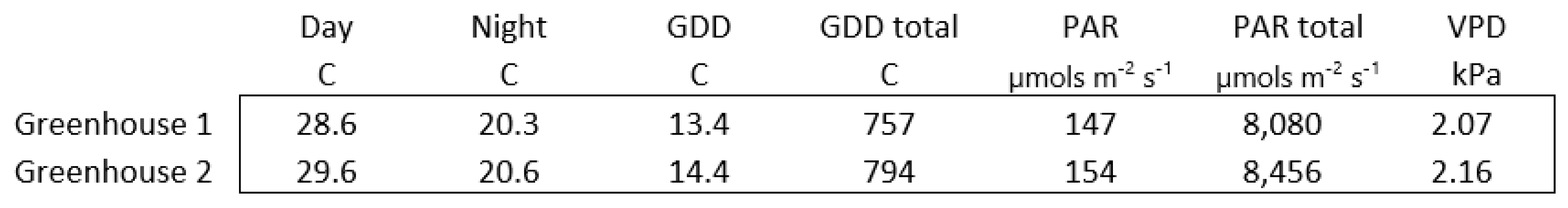
Using a simple methodological approach that involved common inexpensive products, 15.2 × 30.5 cm lysimeter cylindrical containers were assembled from schedule-40 polyvinylchloride pipe and endcaps, then filled with a 10:90 peat to sand ratio USGA (https://www.usga.org/) specification sand (sandy loam) as a growth medium. Plugs of TifTuf Bermuda sod were planted in each container and allowed to establish over a 7-week period. Greenhouse conditions were managed by a Wadsworth Control Systems (Arvada, CO, USA) aspirated temperature controller setting of 33 or 26 °C (day or night respectively). Micro-meteorological conditions were recorded using Campbell Scientific (Campbell Scientific Corporation Logan, UT, USA) data loggers (CR3000 and CR1000x respectively) in each greenhouse and included air temperature and relative humidity measured by the HC2S3 Rotronic sensor (Rotronic Instrument Corp, Hauppauge, NY, USA) nested in an RM Young ten plate solar radiation shield (R.M. Young Comp., Traverse City, MI), full-spectrum solar radiation was measured by the Apogee SP-110 pyranometer, and photosynthetically active radiation with the Apogee SQ-500 quantum sensor (Apogee Instruments, Inc., Logan, UT, USA). At trial initiation, plants were grown in two adjacent greenhouses over eight-week periods and were exposed to 13.4 and 14.4 °C average daily growing degree days (GDD using a base of 10 °C) for a total of 757 and 794 °C GDD respectively. Regarding solar energy, the plants experienced a 150-unit daily average for 4,301 total µmols m^-2 s^-1 photosynthetically active quantum flux radiation (PAR). However, across the experiment period the average daily temperature reduced from 26 to 21 and 28 to 24 °C in the two respective greenhouses, and the PAR reduced from a daily average of 194 to 137 µmols m^-2 s^-1, signifying the autumn seasonal environment.

Table A1. Summary and cummulative environemntal variables that contextualize the growing conditions.

References

J. B. Beard and R. L. Green, “The Role of Turfgrasses in Environmental Protection and Their Benefits to Humans,” J of Env Quality, vol. 23, no. 3, pp. 452–460, 1994. [CrossRef]
P. Niazi, O. Alimyar, A. Azizi, A. W. Monib, and H. Ozturk, “People-plant Interaction: Plant Impact on Humans and Environment,” jeas, vol. 4, no. 2, pp. 01–07, May 2023. [CrossRef]
I. Rehman, B. Hazhirkarzar, and B. C. Patel, “Anatomy, Head and Neck, Eye,” in StatPearls, Treasure Island (FL): StatPearls Publishing, 2024. Accessed: Jun. 14, 2024. [Online]. Available: http://www.ncbi.nlm.nih.gov/books/NBK482428/.
S. Delgado, “Dziga Vertov’s ‘Man with a Movie Camera’ and the Phenomenology of Perception,” Film Criticism, vol. 34, no. 1, pp. 1–16, 2009, Accessed: Jun. 14, 2024. [Online]. Available: https://www.jstor.org/stable/24777403.
M. Wrathall, Skillful Coping: Essays on the Phenomenology of Everyday Perception and Action. Oxford University Press, 2014.
D. Ekdahl, “Review of Daniel O’Shiel, The Phenomenology of Virtual Technology: Perception and Imagination in a Digital Age, Dublin: Bloomsbury Academic, 2022,” Phenom Cogn Sci, pp. s11097-023-09925-y, Jul. 2023. [CrossRef]
R. Sesario, Nugroho Djati Satmoko, Errie Margery, Yusi Faizathul Octavia, and Miska Irani Tarigan, “The Comparison Analysis of Brand Association, Brand Awareness, Brand Loyalty and Perceived Quality of Two Top of Mind Camera Products,” jemsi, vol. 9, no. 2, pp. 388–392, Apr. 2023. [CrossRef]
S. Goma, M. Aleksic, and T. Georgiev, “Camera Technology at the dawn of digital renascence era,” in 2010 Conference Record of the Forty Fourth Asilomar Conference on Signals, Systems and Computers, Nov. 2010, pp. 847–850. [CrossRef]
M. Esposito, M. Crimaldi, V. Cirillo, F. Sarghini, and A. Maggio, “Drone and sensor technology for sustainable weed management: a review,” Chem. Biol. Technol. Agric., vol. 8, no. 1, p. 18, Mar. 2021. [CrossRef]
C. Edwards, R. Nilchiani, A. Ganguly, and M. Vierlboeck, “Evaluating the Tipping Point of a Complex System: The Case of Disruptive Technology.” Sep. 27, 2022. [CrossRef]
X. Yue and E. R. Fossum, “Simulation and design of a burst mode 20Mfps global shutter high conversion gain CMOS image sensor in a standard 180nm CMOS image sensor process using sequential transfer gates,” ei, vol. 35, no. 6, pp. 328-1-328–5, Jan. 2023. [CrossRef]
M. Riccardi, G. Mele, C. Pulvento, A. Lavini, R. d’Andria, and S.-E. Jacobsen, “Non-destructive evaluation of chlorophyll content in quinoa and amaranth leaves by simple and multiple regression analysis of RGB image components,” Photosynth Res, vol. 120, no. 3, pp. 263–272, 2014. [CrossRef]
Y. Chang, S. L. Moan, and D. Bailey, “RGB Imaging Based Estimation of Leaf Chlorophyll Content,” in 2019 International Conference on Image and Vision Computing New Zealand (IVCNZ), Dunedin, New Zealand: IEEE, 2019, pp. 1–6. [CrossRef]
H. Zhang, Y. Ge, X. Xie, A. Atefi, N. K. Wijewardane, and S. Thapa, “High throughput analysis of leaf chlorophyll content in sorghum using RGB, hyperspectral, and fluorescence imaging and sensor fusion,” Plant Methods, vol. 18, no. 1, p. 60, 2022. [CrossRef]
P. Majer, L. Sass, G. V. Horváth, and É. Hideg, “Leaf hue measurements offer a fast, high-throughput initial screening of photosynthesis in leaves,” Journal of Plant Physiology, vol. 167, no. 1, pp. 74–76, 2010. [CrossRef]
I. A. T. F. Taj-Eddin et al., “Can we see photosynthesis? Magnifying the tiny color changes of plant green leaves using Eulerian video magnification,” J. Electron. Imaging, vol. 26, no. 06, p. 1, Nov. 2017. [CrossRef]
M. Vasilev, V. Stoykova, P. Veleva, and Z. Zlatev, “Non-Destructive Determination of Plant Pigments Based on Mobile Phone Data,” TEM Journal, pp. 1430–1442, Aug. 2023. [CrossRef]
S. Kandel et al., “Research directions in data wrangling: Visualizations and transformations for usable and credible data,” Information Visualization, vol. 10, no. 4, pp. 271–288, 2011. [CrossRef]
E. P. White, E. Baldridge, Z. T. Brym, K. J. Locey, D. J. McGlinn, and S. R. Supp, “Nine simple ways to make it easier to (re)use your data,” Ideas in Ecology and Evolution, vol. 6, no. 2, Aug. 2013, Accessed: Jun. 14, 2024. [Online]. Available: https://ojs.library.queensu.ca/index.php/IEE/article/view/4608.
A. Goodman et al., “Ten Simple Rules for the Care and Feeding of Scientific Data,” PLoS Comput Biol, vol. 10, no. 4, p. e1003542, Apr. 2014. [CrossRef]
T. U. Wall, E. McNie, and G. M. Garfin, “Use-inspired science: making science usable by and useful to decision makers,” Frontiers in Ecol & Environ, vol. 15, no. 10, pp. 551–559, 2017. [CrossRef]
D. Gašparovič, J. Žarnovský, H. Beloev, and P. Kangalov, “Evaluation of the Quality of the Photographic Process at the Components Dimensions Measurement,” Agricultural, Forest and Transport Machinery and Technologies, vol. Volume II – Issue 1, no. ISSN: 2367– 5888, 2015, [Online]. Available: https://aftmt.uni-ruse.bg/images/vol.2.1/AFTMT_V_II-1-2015-3.pdf.
G. Liu, S. Tian, Y. Mo, R. Chen, and Q. Zhao, “On the Acquisition of High-Quality Digital Images and Extraction of Effective Color Information for Soil Water Content Testing,” Sensors, vol. 22, no. 9, p. 3130, Apr. 2022. [CrossRef]
D. Chen et al., “Dissecting the Phenotypic Components of Crop Plant Growth and Drought Responses Based on High-Throughput Image Analysis,” The Plant Cell, vol. 26, no. 12, pp. 4636–4655, Jan. 2015. [CrossRef]
N. Honsdorf, T. J. March, B. Berger, M. Tester, and K. Pillen, “High-Throughput Phenotyping to Detect Drought Tolerance QTL in Wild Barley Introgression Lines,” PLoS ONE, vol. 9, no. 5, p. e97047, May 2014. [CrossRef]
Y. Wang, D. Wang, P. Shi, and K. Omasa, “Estimating rice chlorophyll content and leaf nitrogen concentration with a digital still color camera under natural light,” Plant Methods, vol. 10, no. 1, p. 36, 2014. [CrossRef]
K. M. Veley, J. C. Berry, S. J. Fentress, D. P. Schachtman, I. Baxter, and R. Bart, “High-throughput profiling and analysis of plant responses over time to abiotic stress,” Plant Direct, vol. 1, no. 4, p. e00023, 2017. [CrossRef]
Z. Liang et al., “Conventional and hyperspectral time-series imaging of maize lines widely used in field trials,” GigaScience, vol. 7, no. 2, Feb. 2018. [CrossRef]
B. Horvath and J. Vargas Jr, “Analysis of Dollar Spot Disease Severity Using Digital Image Analysis,” International Turfgrass Society Research Journal, vol. Volume 10, pp. 196–201, 2005, [Online]. Available: https://www.researchgate.net/publication/268359230_ANALYSIS_OF_DOLLAR_SPOT_DISEASE_SEVERITY_USING_DIGITAL_IMAGE_ANALYSIS.
F. G. Horgan, A. Jauregui, A. Peñalver Cruz, E. Crisol Martínez, and C. C. Bernal, “Changes in reflectance of rice seedlings during planthopper feeding as detected by digital camera: Potential applications for high-throughput phenotyping,” PLoS ONE, vol. 15, no. 8, p. e0238173, Aug. 2020. [CrossRef]
F. J. Adamsen et al., “Measuring Wheat Senescence with a Digital Camera,” Crop Sci., vol. 39, no. 3, pp. 719–724, 1999. [CrossRef]
J. Friell, E. Watkins, and B. Horgan, “Salt Tolerance of 74 Turfgrass Cultivars in Nutrient Solution Culture,” Crop Science, vol. 53, no. 4, pp. 1743–1749, 2013. [CrossRef]
J. Zhang et al., “Drought responses of above-ground and below-ground characteristics in warm-season turfgrass,” J Agronomy Crop Science, vol. 205, no. 1, pp. 1–12, 2019. [CrossRef]
E. V. Lukina, M. L. Stone, and W. R. Raun, “Estimating vegetation coverage in wheat using digital images,” Journal of Plant Nutrition, vol. 22, no. 2, pp. 341–350, 1999. [CrossRef]
D. E. Karcher and M. D. Richardson, “Batch Analysis of Digital Images to Evaluate Turfgrass Characteristics,” Crop Science, vol. 45, no. 4, pp. 1536–1539, 2005. [CrossRef]
D. J. Bremer, H. Lee, K. Su, and S. J. Keeley, “Relationships between Normalized Difference Vegetation Index and Visual Quality in Cool-Season Turfgrass: II. Factors Affecting NDVI and its Component Reflectances,” Crop Science, vol. 51, no. 5, pp. 2219–2227, 2011. [CrossRef]
B. S. Bushman, B. L. Waldron, J. G. Robins, K. Bhattarai, and P. G. Johnson, “Summer Percent Green Cover among Kentucky Bluegrass Cultivars, Accessions, and Other Poa Species Managed under Deficit Irrigation,” Crop Science, vol. 52, no. 1, pp. 400–407, 2012. [CrossRef]
A. Patrignani and T.E. Ochsner, “Canopeo: A Powerful New Tool for Measuring Fractional Green Canopy Cover,” Agronomy Journal, vol. 107, no. 6, pp. 2312–2320, 2015. [CrossRef]
S. O. Chung, M. S. N. Kabir, and Y. J. Kim, “Variable Fertilizer Recommendation by Image-based Grass Growth Status,” IFAC-PapersOnLine, vol. 51, no. 17, pp. 10–13, 2018. [CrossRef]
K. R. Ball et al., “High-throughput, image-based phenotyping reveals nutrient-dependent growth facilitation in a grass-legume mixture,” PLoS ONE, vol. 15, no. 10, p. e0239673, Oct. 2020. [CrossRef]
H. C. Wright, F. A. Lawrence, A. J. Ryan, and D. D. Cameron, “Free and open-source software for object detection, size, and colour determination for use in plant phenotyping,” Plant Methods, vol. 19, no. 1, p. 126, Nov. 2023. [CrossRef]
J. N. Cobb, G. DeClerck, A. Greenberg, R. Clark, and S. McCouch, “Next-generation phenotyping: requirements and strategies for enhancing our understanding of genotype–phenotype relationships and its relevance to crop improvement,” Theor Appl Genet, vol. 126, no. 4, pp. 867–887, 2013. [CrossRef]
B.T. Gouveia et al., “Multispecies genotype × environment interaction for turfgrass quality in five turfgrass breeding programs in the southeastern United States,” Crop Science, vol. 61, no. 5, pp. 3080–3096, 2021. [CrossRef]
M. F. McCabe and M. Tester, “Digital insights: bridging the phenotype-to-genotype divide,” Journal of Experimental Botany, vol. 72, no. 8, pp. 2807–2810, Apr. 2021. [CrossRef]
M. F. Danilevicz et al., “Plant Genotype to Phenotype Prediction Using Machine Learning,” Front. Genet., vol. 13, p. 822173, May 2022. [CrossRef]
S. A. Tsaftaris, M. Minervini, and H. Scharr, “Machine Learning for Plant Phenotyping Needs Image Processing,” Trends in Plant Science, vol. 21, no. 12, pp. 989–991, 2016. [CrossRef]
U. Lee, S. Chang, G. A. Putra, H. Kim, and D. H. Kim, “An automated, high-throughput plant phenotyping system using machine learning-based plant segmentation and image analysis,” PLoS ONE, vol. 13, no. 4, p. e0196615, Apr. 2018. [CrossRef]
J. C. O. Koh, G. Spangenberg, and S. Kant, “Automated Machine Learning for High-Throughput Image-Based Plant Phenotyping,” Remote Sensing, vol. 13, no. 5, p. 858, Feb. 2021. [CrossRef]
Z. Li, R. Guo, M. Li, Y. Chen, and G. Li, “A review of computer vision technologies for plant phenotyping,” Computers and Electronics in Agriculture, vol. 176, p. 105672, 2020. [CrossRef]
D.T. Smith, A. B. Potgieter, and S. C. Chapman, “Scaling up high-throughput phenotyping for abiotic stress selection in the field,” Theor Appl Genet, vol. 134, no. 6, pp. 1845–1866, 2021. [CrossRef]
L. Li, Q. Zhang, and D. Huang, “A Review of Imaging Techniques for Plant Phenotyping,” Sensors, vol. 14, no. 11, pp. 20078–20111, Oct. 2014. [CrossRef]
Rousseau, H. D. Dee, and T. Pridmore, “Imaging Methods for Phenotyping of Plant Traits,” in Phenomics in Crop Plants: Trends, Options and Limitations, J. Kumar, A. Pratap, and S. Kumar, Eds., New Delhi: Springer India, 2015, pp. 61–74. [CrossRef]
M. Tariq, M. Ahmed, P. Iqbal, Z. Fatima, and S. Ahmad, “Crop Phenotyping,” in Systems Modeling, M. Ahmed, Ed., Singapore: Springer Singapore, 2020, pp. 45–60. [CrossRef]
Cardellicchio; et al. , “Detection of tomato plant phenotyping traits using YOLOv5-based single stage detectors,” Computers and Electronics in Agriculture, vol. 207, p. 107757, 2023. [CrossRef]
N. Harandi, B. Vandenberghe, J. Vankerschaver, S. Depuydt, and A. Van Messem, “How to make sense of 3D representations for plant phenotyping: a compendium of processing and analysis techniques,” Plant Methods, vol. 19, no. 1, p. 60, Jun. 2023. [CrossRef]
C. Zhang, J. Kong, D. Wu, Z. Guan, B. Ding, and F. Chen, “Wearable Sensor: An Emerging Data Collection Tool for Plant Phenotyping,” Plant Phenomics, vol. 5, p. 0051, 2023. [CrossRef]
Y. Zhang and N. Zhang, “Imaging technologies for plant high-throughput phenotyping: a review,” Front. Agr. Sci. Eng., vol. 0, no. 0, p. 0, 2018. [CrossRef]
S. Das Choudhury, A. Samal, and T. Awada, “Leveraging Image Analysis for High-Throughput Plant Phenotyping,” Front. Plant Sci., vol. 10, p. 508, Apr. 2019. [CrossRef]
Department of Computer Science and IT, N.M.S. Sermathai Vasan College for Women, Madurai, India. and K. Rani, “Image Analysis Techniqueson Phenotype for Plant System,” IJEAT, vol. 9, no. 1s4, pp. 565–568, Dec. 2019. [CrossRef]
M. Kamran Omari, J. Lee, M. Akbar Faqeerzada, R. Joshi, E. Park, and B.-K. Cho, “Digital image-based plant phenotyping: a review,” Korean Journal of Agricultural Science, vol. 47(1), pp. 119–130, 2020, [Online]. Available: https://www.researchgate.net/publication/340032840_Digital_image-based_plant_phenotyping_a_review.
H. L. Shantz, “The Place of Grasslands in the Earth’s Cover,” Ecology, vol. 35, no. 2, pp. 143–145, 1954. [CrossRef]
B. F. Jacobs, J. D. Kingston, and L. L. Jacobs, “The Origin of Grass-Dominated Ecosystems,” Annals of the Missouri Botanical Garden, vol. 86, no. 2, pp. 590–643, 1999. [CrossRef]
A. R. Watkinson and S. J. Ormerod, “Grasslands, Grazing and Biodiversity: Editors’ Introduction,” Journal of Applied Ecology, vol. 38, no. 2, pp. 233–237, 2001, Accessed: Jun. 14, 2024. [Online]. Available: https://www.jstor.org/stable/2655793.
C. A. E. Strömberg, “Evolution of Grasses and Grassland Ecosystems,” Annu. Rev. Earth Planet. Sci., vol. 39, no. 1, pp. 517–544, May 2011. https://doi.org/10.1146/annurev-earth-040809-152402. [CrossRef]
S. L. Chawla, M. A. Roshni Agnihotri, P. Sudha, and H. P. Shah, “Turfgrass: A Billion Dollar Industry,” in National Conference on Floriculture for Rural and Urban Prosperity in the Scenario of Climate Change, 2018. [Online]. Available: https://www.researchgate.net/publication/324483293_Turfgrass_A_Billion_Dollar_Industry.
J. Wu and M. E. Bauer, “Estimating Net Primary Production of Turfgrass in an Urban-Suburban Landscape with QuickBird Imagery,” Remote Sensing, vol. 4, no. 4, pp. 849–866, Mar. 2012. [CrossRef]
Milesi, S. W. Running, C. D. Elvidge, J. B. Dietz, B. T. Tuttle, and R. R. Nemani, “Mapping and Modeling the Biogeochemical Cycling of Turf Grasses in the United States,” Environmental Management, vol. 36, no. 3, pp. 426–438, 2005. [CrossRef]
C. A. Blanco-Montero, T. B. Bennett, P. Neville, C. S. Crawford, B. T. Milne, and C. R. Ward, “Potential environmental and economic impacts of turfgrass in Albuquerque, New Mexico (USA),” Landscape Ecol, vol. 10, no. 2, pp. 121–128, 1995. [CrossRef]
J. V. Krans and K. Morris, “Determining a Profile of Protocols and Standards used in the Visual Field Assessment of Turfgrasses: A Survey of National Turfgrass Evaluation Program-Sponsored University Scientists,” Applied Turfgrass Science, vol. 4, no. 1, pp. 1–6, 2007. [CrossRef]
J. B. Beard, Turfgrass: Science and culture. Englewood Cliffs, NJ: Prentice Hall, 1973. [Online]. Available: https://catalogue.nla.gov.au/catalog/2595129.
A. Calera, C. Martínez, and J. Melia, “A procedure for obtaining green plant cover: Relation to NDVI in a case study for barley,” International Journal of Remote Sensing, vol. 22, no. 17, pp. 3357–3362, 2001. [CrossRef]
L. Cabrera-Bosquet, G. Molero, A. Stellacci, J. Bort, S. Nogués, and J. Araus, “NDVI as a potential tool for predicting biomass, plant nitrogen content and growth in wheat genotypes subjected to different water and nitrogen conditions,” Cereal Research Communications, vol. 39, no. 1, pp. 147–159, 2011. [CrossRef]
R. L. Rorie et al., “Association of ‘Greenness’ in Corn with Yield and Leaf Nitrogen Concentration,” Agronomy Journal, vol. 103, no. 2, pp. 529–535, 2011. [CrossRef]
M. OZYAVUZ, B. C. BILGILI, and S. SALICI, “Determination of Vegetation Changes with NDVI Method,” Journal of Environmental Protection and Ecology, vol. 16, no. 1, pp. 264–273, 2015, [Online]. Available: https://www.researchgate.net/publication/284981527_Determination_of_vegetation_changes_with_NDVI_method.
S. Huang, L. Tang, J. P. Hupy, Y. Wang, and G. Shao, “A commentary review on the use of normalized difference vegetation index (NDVI) in the era of popular remote sensing,” J. For. Res., vol. 32, no. 1, pp. 1–6, 2021. [CrossRef]
Y. Xu, Y. Yang, X. Chen, and Y. Liu, “Bibliometric Analysis of Global NDVI Research Trends from 1985 to 2021,” Remote Sensing, vol. 14, no. 16, p. 3967, Aug. 2022. [CrossRef]
T. N. Carlson and D. A. Ripley, “On the relation between NDVI, fractional vegetation cover, and leaf area index,” Remote Sensing of Environment, vol. 62, no. 3, pp. 241–252, 1997. [CrossRef]
T. R. Tenreiro, M. García-Vila, J. A. Gómez, J. A. Jiménez-Berni, and E. Fereres, “Using NDVI for the assessment of canopy cover in agricultural crops within modelling research,” Computers and Electronics in Agriculture, vol. 182, p. 106038, 2021. [CrossRef]
P. V. Lykhovyd, R. A. Vozhehova, S. O. Lavrenko, and N. M. Lavrenko, “The Study on the Relationship between Normalized Difference Vegetation Index and Fractional Green Canopy Cover in Five Selected Crops,” The Scientific World Journal, vol. 2022, pp. 1–6, Mar. 2022. [CrossRef]
M. Pagola et al., “New method to assess barley nitrogen nutrition status based on image colour analysis,” Computers and Electronics in Agriculture, vol. 65, no. 2, pp. 213–218, 2009. [CrossRef]
C. M. Straw and G. M. Henry, “Spatiotemporal variation of site-specific management units on natural turfgrass sports fields during dry down,” Precision Agric, vol. 19, no. 3, pp. 395–420, 2018. [CrossRef]
R. Hejl, C. Straw, B. Wherley, R. Bowling, and K. McInnes, “Factors leading to spatiotemporal variability of soil moisture and turfgrass quality within sand-capped golf course fairways,” Precision Agric, vol. 23, no. 5, pp. 1908–1917, 2022. [CrossRef]
S. Kawashima, “An Algorithm for Estimating Chlorophyll Content in Leaves Using a Video Camera,” Annals of Botany, vol. 81, no. 1, pp. 49–54, 1998. [CrossRef]
E. R. Hunt, P. C. Doraiswamy, J. E. McMurtrey, C. S. T. Daughtry, E. M. Perry, and B. Akhmedov, “A visible band index for remote sensing leaf chlorophyll content at the canopy scale,” International Journal of Applied Earth Observation and Geoinformation, vol. 21, pp. 103–112, 2013. [CrossRef]
M. Schiavon, B. Leinauer, E. Sevastionova, M. Serena, and B. Maier, “Warm-season Turfgrass Quality, Spring Green-up, and Fall Color Retention under Drip Irrigation,” Applied Turfgrass Science, vol. 8, no. 1, pp. 1–9, 2011. [CrossRef]
J. Marín, S. Yousfi, P. V. Mauri, L. Parra, J. Lloret, and A. Masaguer, “RGB Vegetation Indices, NDVI, and Biomass as Indicators to Evaluate C3 and C4 Turfgrass under Different Water Conditions,” Sustainability, vol. 12, no. 6, p. 2160, Mar. 2020. [CrossRef]
G. E. Bell et al., “Vehicle-Mounted Optical Sensing: An Objective Means for Evaluating Turf Quality,” Crop Science, vol. 42, no. 1, pp. 197–201, 2002. [CrossRef]
G. E. Bell, D. L. Martin, K. Koh, and H. R. Han, “Comparison of Turfgrass Visual Quality Ratings with Ratings Determined Using a Handheld Optical Sensor,” hortte, vol. 19, no. 2, pp. 309–316, 2009. [CrossRef]
D. E. Karcher and M. D. Richardson, “Digital Image Analysis in Turfgrass Research,” in Turfgrass: Biology, Use, and Management, J. C. Stier, B. P. Horgan, and S. A. Bonos, Eds., Madison, WI, USA: American Society of Agronomy, Crop Science Society of America, Soil Science Society of America, 2015, pp. 1133-1149–2. [CrossRef]
B. D. S. Barbosa et al., “RGB vegetation indices applied to grass monitoring: a qualitative analysis,” p. 675.9Kb, 2019. [CrossRef]
B. Whitman, B. V. Iannone, J. K. Kruse, J. B. Unruh, and A. G. Dale, “Cultivar blends: A strategy for creating more resilient warm season turfgrass lawns,” Urban Ecosyst, vol. 25, no. 3, pp. 797–810, 2022. [CrossRef]
D. Hahn, A. Morales, C. Velasco-Cruz, and B. Leinauer, “Assessing Competitiveness of Fine Fescues (Festuca L. spp.) and Tall Fescue (Schedonorus arundinaceous (Schreb.) Dumort) Established with White Clover (Trifolium repens L., WC), Daisy (Bellis perennis L.) and Yarrow (Achillea millefolium L.),” Agronomy, vol. 11, no. 11, p. 2226, Nov. 2021. [CrossRef]
B. Schwartz, J. Zhang, J. Fox, and J. Peake, “Turf Performance of Shaded ‘TifGrand’ and ‘TifSport’ Hybrid Bermudagrass as Affected by Mowing Height and Trinexapac-ethyl,” hortte, vol. 30, no. 3, pp. 391–397, 2020. [CrossRef]
M. D. Richardson, D. E. Karcher, A. J. Patton, and J. H. McCalla, “Measurement of Golf Ball Lie in Various Turfgrasses Using Digital Image Analysis,” Crop Science, vol. 50, no. 2, pp. 730–736, 2010. [CrossRef]
A. Walter, B. Studer, and R. Kölliker, “Advanced phenotyping offers opportunities for improved breeding of forage and turf species,” Annals of Botany, vol. 110, no. 6, pp. 1271–1279, 2012. [CrossRef]
J. B. Hu, M. X. Dai, and S. T. Peng, “An automated (novel) algorithm for estimating green vegetation cover fraction from digital image: UIP-MGMEP,” Environ Monit Assess, vol. 190, no. 11, p. 687, 2018. [CrossRef]
P. Xu, N. Wang, X. Zheng, G. Qiu, and B. Luo, “A New Turfgrass Coverage Evaluation Method Based on Two-Stage k-means Color Classifier,” in 2019 Boston, Massachusetts July 7- July 10, 2019, American Society of Agricultural and Biological Engineers, 2019. [CrossRef]
S. Xie, C. Hu, M. Bagavathiannan, and D. Song, “Toward Robotic Weed Control: Detection of Nutsedge Weed in Bermudagrass Turf Using Inaccurate and Insufficient Training Data,” IEEE Robot. Autom. Lett., vol. 6, no. 4, pp. 7365–7372, 2021. [CrossRef]
J. B. Ortiz, C. N. Hirsch, N. J. Ehlke, and E. Watkins, “SpykProps: an imaging pipeline to quantify architecture in unilateral grass inflorescences,” Plant Methods, vol. 19, no. 1, p. 125, Nov. 2023. [CrossRef]
D. J. Bremer, H. Lee, K. Su, and S. J. Keeley, “Relationships between Normalized Difference Vegetation Index and Visual Quality in Cool-Season Turfgrass: I. Variation among Species and Cultivars,” Crop Science, vol. 51, no. 5, pp. 2212–2218, 2011. [CrossRef]
H.Lee, D. J. Bremer, K. Su, and S. J. Keeley, “Relationships between Normalized Difference Vegetation Index and Visual Quality in Turfgrasses: Effects of Mowing Height,” Crop Science, vol. 51, no. 1, pp. 323–332, 2011. [CrossRef]
B.Leinauer, D. M. VanLeeuwen, M. Serena, M. Schiavon, and E. Sevostianova, “Digital Image Analysis and Spectral Reflectance to Determine Turfgrass Quality,” Agronomy Journal, vol. 106, no. 5, pp. 1787–1794, 2014. [CrossRef]
A.Haghverdi, A. Sapkota, A. Singh, S. Ghodsi, and M. Reiter, “Developing Turfgrass Water Response Function and Assessing Visual Quality, Soil Moisture and NDVI Dynamics of Tall Fescue Under Varying Irrigation Scenarios in Inland Southern California,” Journal of the ASABE, vol. 66, no. 6, pp. 1497–1512, 2023. [CrossRef]
R. W. Hejl, M. M. Conley, D. D. Serba, and C. F. Williams, “Mowing Height Effects on ‘TifTuf’ Bermudagrass during Deficit Irrigation,” Agronomy, vol. 14, no. 3, p. 628, Mar. 2024. [CrossRef]
B.Boiarskii, “Comparison of NDVI and NDRE Indices to Detect Differences in Vegetation and Chlorophyll Content,” JMCMS, vol. spl1, no. 4, Nov. 2019. [CrossRef]
F.Pallottino, F. Antonucci, C. Costa, C. Bisaglia, S. Figorilli, and P. Menesatti, “Optoelectronic proximal sensing vehicle-mounted technologies in precision agriculture: A review,” Computers and Electronics in Agriculture, vol. 162, pp. 859–873, 2019. [CrossRef]
R. K. Kurbanov and N. I. Zakharova, “Application of Vegetation Indexes to Assess the Condition of Crops,” S-h. maš. tehnol., vol. 14, no. 4, pp. 4–11, Dec. 2020. [CrossRef]
J.Frossard and, O. Renaud, “Permutation Tests for Regression, ANOVA, and Comparison of Signals: The permuco Package,” J. Stat. Soft., vol. 99, no. 15, 2021. [CrossRef]
M. D. Richardson, D. E. Karcher, and L. C. Purcell, “Quantifying Turfgrass Cover Using Digital Image Analysis,” Crop Science, vol. 41, no. 6, pp. 1884–1888, 2001. [CrossRef]
C.Zhang, G. D. Pinnix, Z. Zhang, G. L. Miller, and T. W. Rufty, “Evaluation of Key Methodology for Digital Image Analysis of Turfgrass Color Using Open-Source Software,” Crop Science, vol. 57, no. 2, pp. 550–558, 2017. [CrossRef]
M. S. Woolf, L. M. Dignan, A. T. Scott, and J. P. Landers, “Digital postprocessing and image segmentation for objective analysis of colorimetric reactions,” Nat Protoc, vol. 16, no. 1, pp. 218–238, 2021. [CrossRef]
D.E. Karcher and M. D. Richardson, “Quantifying Turfgrass Color Using Digital Image Analysis,” Crop Science, vol. 43, no. 3, pp. 943–951, 2003. [CrossRef]
M. Anderson, R. Motta, S. Chandrasekar, and M. Stokes, “Proposal for a Standard Default Color Space for the Internet—sRGB,” in The Fourth Color Imaging Conference, Society of Imaging Science and Technology, 1996, pp. 239–245. [Online]. Available: https://library.imaging.org/admin/apis/public/api/ist/website/downloadArticle/cic/4/1/art00061.
J. Casadesús and, D. Villegas, “Conventional digital cameras as a tool for assessing leaf area index and biomass for cereal breeding,” JIPB, vol. 56, no. 1, pp. 7–14, 2014. [CrossRef]
D.Karcher, C. Purcell, and K. Hignight, “Devices, systems and methods for digital image analysis,” US20220270206A1, Aug. 25, 2022 Accessed: Jun. 14, 2024. [Online]. Available: https://patents.google.com/patent/US20220270206A1/en.
M. Schiavon, B. Leinauer, M. Serena, R. Sallenave, and B. Maier, “Establishing Tall Fescue and Kentucky Bluegrass Using Subsurface Irrigation and Saline Water,” Agronomy Journal, vol. 105, no. 1, pp. 183–190, 2013. [CrossRef]
M. Giolo, C. Pornaro, A. Onofri, and S. Macolino, “Seeding Time Affects Bermudagrass Establishment in the Transition Zone Environment,” Agronomy, vol. 10, no. 8, p. 1151, Aug. 2020. [CrossRef]
M. Schiavon, C. Pornaro, and S. Macolino, “Tall Fescue (Schedonorus arundinaceus (Schreb.) Dumort.) Turfgrass Cultivars Performance under Reduced N Fertilization,” Agronomy, vol. 11, no. 2, p. 193, Jan. 2021. [CrossRef]
B.Zhao et al., “Estimating the Growth Indices and Nitrogen Status Based on Color Digital Image Analysis During Early Growth Period of Winter Wheat,” Front. Plant Sci., vol. 12, p. 619522, Apr. 2021. [CrossRef]
A. Sierra Augustinus, P. H. McLoughlin, A. F. Arevalo Alvarenga, J. B. Unruh, and M. Schiavon, “Evaluation of Different Aerification Methods for Ultradwarf Hybrid Bermudagrass Putting Greens,” hortte, vol. 33, no. 4, pp. 333–341, 2023. [CrossRef]
S. Singh et al., “Genetic Variability of Traffic Tolerance and Surface Playability of Bermudagrass (Cynodon spp.) under Fall Simulated Traffic Stress,” horts, vol. 59, no. 1, pp. 73–83, 2024. [CrossRef]
T. Glab, W. Szewczyk, and K. Gondek, “Response of Kentucky Bluegrass Turfgrass to Plant Growth Regulators,” Agronomy, vol. 13, no. 3, p. 799, Mar. 2023. [CrossRef]
M. Guijarro, G. Pajares, I. Riomoros, P. J. Herrera, X. P. Burgos-Artizzu, and A. Ribeiro, “Automatic segmentation of relevant textures in agricultural images,” Computers and Electronics in Agriculture, vol. 75, no. 1, pp. 75–83, Jan. 2011. [CrossRef]
D.M. Woebbecke, G. E. Meyer, K. Von Bargen, and D. A. Mortensen, “Color Indices for Weed Identification Under Various Soil, Residue, and Lighting Conditions,” Transactions of the ASAE, vol. 38, no. 1, pp. 259–269, 1995. [CrossRef]
T. Kataoka, T. Kaneko, H. Okamoto, and S. Hata, “Crop growth estimation system using machine vision,” in Proceedings 2003 IEEE/ASME International Conference on Advanced Intelligent Mechatronics (AIM 2003), Kobe, Japan: IEEE, 2003, pp. b1079–b1083. [CrossRef]
J.A. Marchant and C. M. Onyango, “Shadow-invariant classification for scenes illuminated by daylight,” J. Opt. Soc. Am. A, JOSAA, vol. 17, no. 11, pp. 1952–1961, Nov. 2000. [CrossRef]
T. Hague, N. D. Tillett, and H. Wheeler, “Automated Crop and Weed Monitoring in Widely Spaced Cereals,” Precision Agric, vol. 7, no. 1, pp. 21–32, Mar. 2006. [CrossRef]
R. Robertson, “The CIE 1976 Color-Difference Formulae,” Color Research & Application, vol. 2, no. 1, pp. 7–11, 1977. [CrossRef]
J. Schwiegerling, Field Guide to Visual and Ophthalmic Optics, vol. FG04. Bellingham, Washington, USA: SPIE, 2004. [Online]. Available: https://spie.org/publications/spie-publication-resources/optipedia-free-optics-information/fg04_p12_phoscoresponse?
A. Koschan and M., A. Abidi, Digital Color Image Processing, 1st ed. Wiley, 2008. [CrossRef]
J. Chopin, P. Kumar, and S. J. Miklavcic, “Land-based crop phenotyping by image analysis: consistent canopy characterization from inconsistent field illumination,” Plant Methods, vol. 14, no. 1, p. 39, 2018. [CrossRef]
J.M. Pape and C. Klukas, “Utilizing machine learning approaches to improve the prediction of leaf counts and individual leaf segmentation of rosette plant images,” Department of Molecular Genetics, Leibniz Institute of Plant Genetics and Crop Plant Research (IPK), 06466 Gatersleben, Germany, 2015. [Online]. Available: https://openimageanalysisgroup.github.io/MCCCS/publications/Pape_Klukas_LSC_2015.pdf.
S. C. Kefauver et al., “Comparative UAV and Field Phenotyping to Assess Yield and Nitrogen Use Efficiency in Hybrid and Conventional Barley,” Front. Plant Sci., vol. 8, p. 1733, Oct. 2017. [CrossRef]
J. Du, B. Li, X. Lu, X. Yang, X. Guo, and C. Zhao, “Quantitative phenotyping and evaluation for lettuce leaves of multiple semantic components,” Plant Methods, vol. 18, no. 1, p. 54, 2022. [CrossRef]
X. Xie et al., “A Novel Feature Selection Strategy Based on Salp Swarm Algorithm for Plant Disease Detection,” Plant Phenomics, vol. 5, p. 0039, 2023. [CrossRef]
W. Wahono, D. Indradewa, B. H. Sunarminto, E. Haryono, and D. Prajitno, “CIE L*a*b* Color Space Based Vegetation Indices Derived from Unmanned Aerial Vehicle Captured Images for Chlorophyll and Nitrogen Content Estimation of Tea (Camellia sinensis L. Kuntze) Leaves,” Ilmu Pertanian (Agricultural Science), vol. 4, no. 1, pp. 46–51, May 2019. [CrossRef]
R. R. De Casas, P. Vargas, E. Pérez-Corona, E. Manrique, C. García-Verdugo, and L. Balaguer, “Sun and shade leaves of Olea europaea respond differently to plant size, light availability and genetic variation: Canopy plasticity in Olea europea,” Functional Ecology, vol. 25, no. 4, pp. 802–812, 2011. [CrossRef]
S. Rasmann, E. Chassin, J. Bilat, G. Glauser, and P. Reymond, “Trade-off between constitutive and inducible resistance against herbivores is only partially explained by gene expression and glucosinolate production,” Journal of Experimental Botany, vol. 66, no. 9, pp. 2527–2534, 2015. [CrossRef]
J. C. Berry et al., “Increased signal-to-noise ratios within experimental field trials by regressing spatially distributed soil properties as principal components,” eLife, vol. 11, p. e70056, Jul. 2022. [CrossRef]
E. Fitz–Rodríguez and C., Y. Choi, “Monitoring Turfgrass Quality Using Multispectral Radiometry,” Transactions of the ASAE, vol. 45, no. 3, 2002. [CrossRef]
H.M. Aynalem, T. L. Righetti, and B. M. Reed, “Non-destructive evaluation of in vitro-stored plants: A comparison of visual and image analysis,” In Vitro Cell. Dev. Biol. - Plant, vol. 42, no. 6, pp. 562–567, 2006. [CrossRef]
A.S. Kaler et al., “Genome-Wide Association Mapping of Dark Green Color Index using a Diverse Panel of Soybean Accessions,” Sci Rep, vol. 10, no. 1, p. 5166, Mar. 2020. [CrossRef]
M.S. Brown, “Color Processing for Digital Cameras,” in Fundamentals and Applications of Colour Engineering, 1st ed., P. Green, Ed., Wiley, 2023, pp. 81–98. [CrossRef]
J. Casadesús et al., “Using vegetation indices derived from conventional digital cameras as selection criteria for wheat breeding in water-limited environments,” Annals of Applied Biology, vol. 150, no. 2, pp. 227–236, 2007. [CrossRef]
K. W. Houser, M. Wei, A. David, M. R. Krames, and X. S. Shen, “Review of measures for light-source color rendition and considerations for a two-measure system for characterizing color rendition,” Opt. Express, vol. 21, no. 8, p. 10393, Apr. 2013. [CrossRef]
W. L. Wu et al., “High Color Rendering Index of Rb 2 GeF 6 :Mn 4+ for Light-Emitting Diodes,” Chem. Mater., vol. 29, no. 3, pp. 935–939, Feb. 2017. [CrossRef]
J. Schewe, The Digital Negative: Raw Image Processing in Lightroom, Camera Raw, and Photoshop. Peachpit Pr, 2012.
S. H. Lee and J. S. Choi, “Design and implementation of color correction system for images captured by digital camera,” IEEE Trans. Consumer Electron., vol. 54, no. 2, pp. 268–276, 2008. [CrossRef]
G. D. Finlayson, M. Mackiewicz, and A. Hurlbert, “Color Correction Using Root-Polynomial Regression,” IEEE Trans. on Image Process., vol. 24, no. 5, pp. 1460–1470, 2015. [CrossRef]
V. Senthilkumaran, “Color Correction Using Color Checkers,” presented at the Proceedings of the First International Conference on Combinatorial and Optimization, ICCAP 2021, December 7-8 2021, Chennai, India, Dec. 2021. Accessed: Jun. 14, 2024. [Online]. Available: https://eudl.eu/doi/10.4108/eai.7-12-2021.2314537.
D. Okkalides, “Assessment of commercial compression algorithms, of the lossy DCT and lossless types, applied to diagnostic digital image files,” Computerized Medical Imaging and Graphics, vol. 22, no. 1, pp. 25–30, 1998. [CrossRef]
V. Lebourgeois, A. Bégué, S. Labbé, B. Mallavan, L. Prévot, and B. Roux, “Can Commercial Digital Cameras Be Used as Multispectral Sensors? A Crop Monitoring Test,” Sensors, vol. 8, no. 11, pp. 7300–7322, Nov. 2008. [CrossRef]
A. Zabala and, X. Pons, “Effects of lossy compression on remote sensing image classification of forest areas,” International Journal of Applied Earth Observation and Geoinformation, vol. 13, no. 1, pp. 43–51, 2011. [CrossRef]
A. Zabala and, X. Pons, “Impact of lossy compression on mapping crop areas from remote sensing,” International Journal of Remote Sensing, vol. 34, no. 8, pp. 2796–2813, Apr. 2013. [CrossRef]
J. Casadesús, C. Biel, and R. Savé, “Turf color measurement with conventional digital cameras,” in Vila Real, Universidade de Trás-os-Montes e Alto Douro, 2005.
Ku, S. Mansoor, G. D. Han, Y. S. Chung, and T. T. Tuan, “Identification of new cold tolerant Zoysia grass species using high-resolution RGB and multi-spectral imaging,” Sci Rep, vol. 13, no. 1, p. 13209, Aug. 2023. [CrossRef]
S. S. Mutlu, N. K. Sönmez, M. Çoşlu, H. R. Türkkan, and D. Zorlu, “UAV-based imaging for selection of turfgrass drought resistant cultivars in breeding trials,” Euphytica, vol. 219, no. 8, p. 83, 2023. [CrossRef]
R. Matsuoka, K. Asonuma, G. Takahashi, T. Danjo, and K. Hirana, “Evaluation of Correction Methods of Chromatic Aberration in Digital Camera Images,” ISPRS Ann. Photogramm. Remote Sens. Spatial Inf. Sci., vol. I–3, pp. 49–55, Jul. 2012. [CrossRef]
M. Mackiewicz, C. F. Andersen, and G. Finlayson, “Method for hue plane preserving color correction,” J. Opt. Soc. Am. A, vol. 33, no. 11, p. 2166, Nov. 2016. [CrossRef]
J. C. Berry, N. Fahlgren, A. A. Pokorny, R. S. Bart, and K. M. Veley, “An automated, high-throughput method for standardizing image color profiles to improve image-based plant phenotyping,” PeerJ, vol. 6, p. e5727, Oct. 2018. [CrossRef]
O. Burggraaff et al., “Standardized spectral and radiometric calibration of consumer cameras,” Opt. Express, vol. 27, no. 14, p. 19075, Jul. 2019. [CrossRef]
L. Tu, Q. Peng, C. Li, and A. Zhang, “2D In Situ Method for Measuring Plant Leaf Area with Camera Correction and Background Color Calibration,” Scientific Programming, vol. 2021, pp. 1–11, Mar. 2021. [CrossRef]
D. Lozano-Claros, E. Custovic, G. Deng, J. Whelan, and M. G. Lewsey, “ColorBayes: Improved color correction of high-throughput plant phenotyping images to account for local illumination differences.” Mar. 02, 2022. [CrossRef]
J. Chopin, P. Kumar, and S. J. Miklavcic, “Land-based crop phenotyping by image analysis: consistent canopy characterization from inconsistent field illumination,” Plant Methods, vol. 14, no. 1, p. 39, May 2018. [CrossRef]
Y. Liang, D. Urano, K.-L. Liao, T. L. Hedrick, Y. Gao, and A. M. Jones, “A nondestructive method to estimate the chlorophyll content of Arabidopsis seedlings,” Plant Methods, vol. 13, no. 1, p. 26, 2017. [CrossRef]
J. C. O. Koh, M. Hayden, H. Daetwyler, and S. Kant, “Estimation of crop plant density at early mixed growth stages using UAV imagery,” Plant Methods, vol. 15, no. 1, p. 64, 2019. [CrossRef]
W. H. Ryan et al., “The Use of Photographic Color Information for High-Throughput Phenotyping of Pigment Composition in Agarophyton vermiculophyllum (Ohmi) Gurgel, J.N.Norris & Fredericq,” Cryptogamie, Algologie, vol. 40, no. 7, p. 73, Sep. 2019. [CrossRef]
I. Borra-Serrano, A. Kemeltaeva, K. Van Laere, P. Lootens, and L. Leus, “A view from above: can drones be used for image-based phenotyping in garden rose breeding?,” Acta Hortic., no. 1368, pp. 271–280, 2023. [CrossRef]
W. Yin, X. Zang, L. Wu, X. Zhang, and J. Zhao, “A Distortion Correction Method Based on Actual Camera Imaging Principles,” Sensors, vol. 24, no. 8, p. 2406, Apr. 2024. [CrossRef]
J. F. Paril and A. J. Fournier-Level, “instaGraminoid, a Novel Colorimetric Method to Assess Herbicide Resistance, Identifies Patterns of Cross-Resistance in Annual Ryegrass,” Plant Phenomics, vol. 2019, p. 2019/7937156, 2019. [CrossRef]
P. L. Vines, J. Zhang, P. L. Vines, and J. Zhang, “High-throughput plant phenotyping for improved turfgrass breeding applications,” G, vol. 2, no. 1, pp. 1–13, Jan. 2022. [CrossRef]
T. Wang, A. Chandra, J. Jung, and A. Chang, “UAV remote sensing based estimation of green cover during turfgrass establishment,” Computers and Electronics in Agriculture, vol. 194, p. 106721, 2022. [CrossRef]
A. Atefi, Y. Ge, S. Pitla, and J. Schnable, “In vivo human-like robotic phenotyping of leaf traits in maize and sorghum in greenhouse,” Computers and Electronics in Agriculture, vol. 163, p. 104854, 2019. [CrossRef]
A. Atefi, Y. Ge, S. Pitla, and J. Schnable, “Robotic Technologies for High-Throughput Plant Phenotyping: Contemporary Reviews and Future Perspectives,” Front. Plant Sci., vol. 12, p. 611940, Jun. 2021. [CrossRef]
A. Arunachalam and, H. Andreasson, “Real-time plant phenomics under robotic farming setup: A vision-based platform for complex plant phenotyping tasks,” Computers & Electrical Engineering, vol. 92, p. 107098, 2021. [CrossRef]
H. Fonteijn et al., “Automatic Phenotyping of Tomatoes in Production Greenhouses Using Robotics and Computer Vision: From Theory to Practice,” Agronomy, vol. 11, no. 8, p. 1599, Aug. 2021. [CrossRef]
L. Yao, R. Van De Zedde, and G. Kowalchuk, “Recent developments and potential of robotics in plant eco-phenotyping,” Emerging Topics in Life Sciences, vol. 5, no. 2, pp. 289–300, May 2021. [CrossRef]
S. Pongpiyapaiboon et al., “Development of a digital phenotyping system using 3D model reconstruction for zoysiagrass,” The Plant Phenome Journal, vol. 6, no. 1, p. e20076, 2023. [CrossRef]
H. Bethge, T. Winkelmann, P. Lüdeke, and T. Rath, “Low-cost and automated phenotyping system ‘Phenomenon’ for multi-sensor in situ monitoring in plant in vitro culture,” Plant Methods, vol. 19, no. 1, p. 42, May 2023. [CrossRef]
K. Ma, X. Cui, G. Huang, and D. Yuan, “Effect of Light Intensity on Close-Range Photographic Imaging Quality and Measurement Precision,” IJMUE, vol. 11, no. 2, pp. 69–78, Feb. 2016. [CrossRef]
J. Bendig, D. Gautam, Z. Malenovsky, and A. Lucieer, “Influence of Cosine Corrector and Uas Platform Dynamics on Airborne Spectral Irradiance Measurements,” in IGARSS 2018 - 2018 IEEE International Geoscience and Remote Sensing Symposium, Valencia: IEEE, 2018, pp. 8822–8825. [CrossRef]
Z. Feng, Q. Liang, Z. Zhang, and W. Ji, “Camera Calibration Method Based on Sine Cosine Algorithm,” in 2021 IEEE International Conference on Progress in Informatics and Computing (PIC), Shanghai, China: IEEE, Dec. 2021, pp. 174–178. [CrossRef]

Figure 3. NDVI time series chart with NDVI plotted on the Y-axis and date on the X-axis. The experimental treatments are labeled by their percentage of consumptive demand-based irrigation supplied (i = 100, 65, & 30) and their mowing heights (h = 10, 7.5, 5.0, & 2.5 cm). Each treatment is grouped by irrigation level and uniquely colored, the line pattern is based on mowing height. NDVI shows changes in time and differences with experimental treatment.

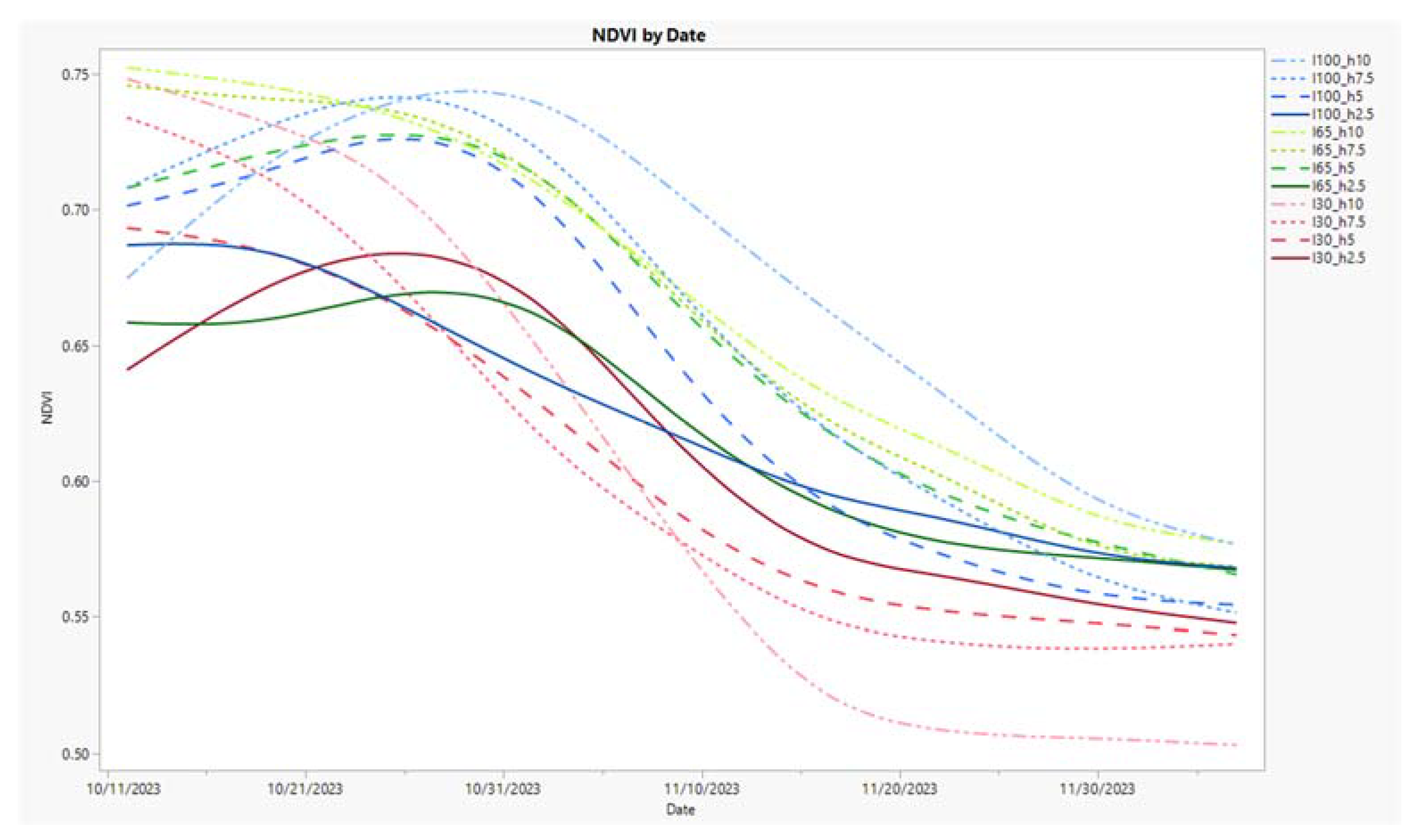
Figure 4. %Y time series chart where the image-based yellow color classification segment is plotted on the inverted Y-axis and the date is on the X-axis. The experimental treatments are labeled by their percentage of consumptive demand-based irrigation supplied (i = 100, 65, & 30) and their mowing heights (h = 10, 7.5, 5.0, & 2.5 cm). Each treatment is grouped by irrigation level and uniquely colored, the line pattern is based on mowing height. Results show change over time and increased treatment separations with greatly reduced water.

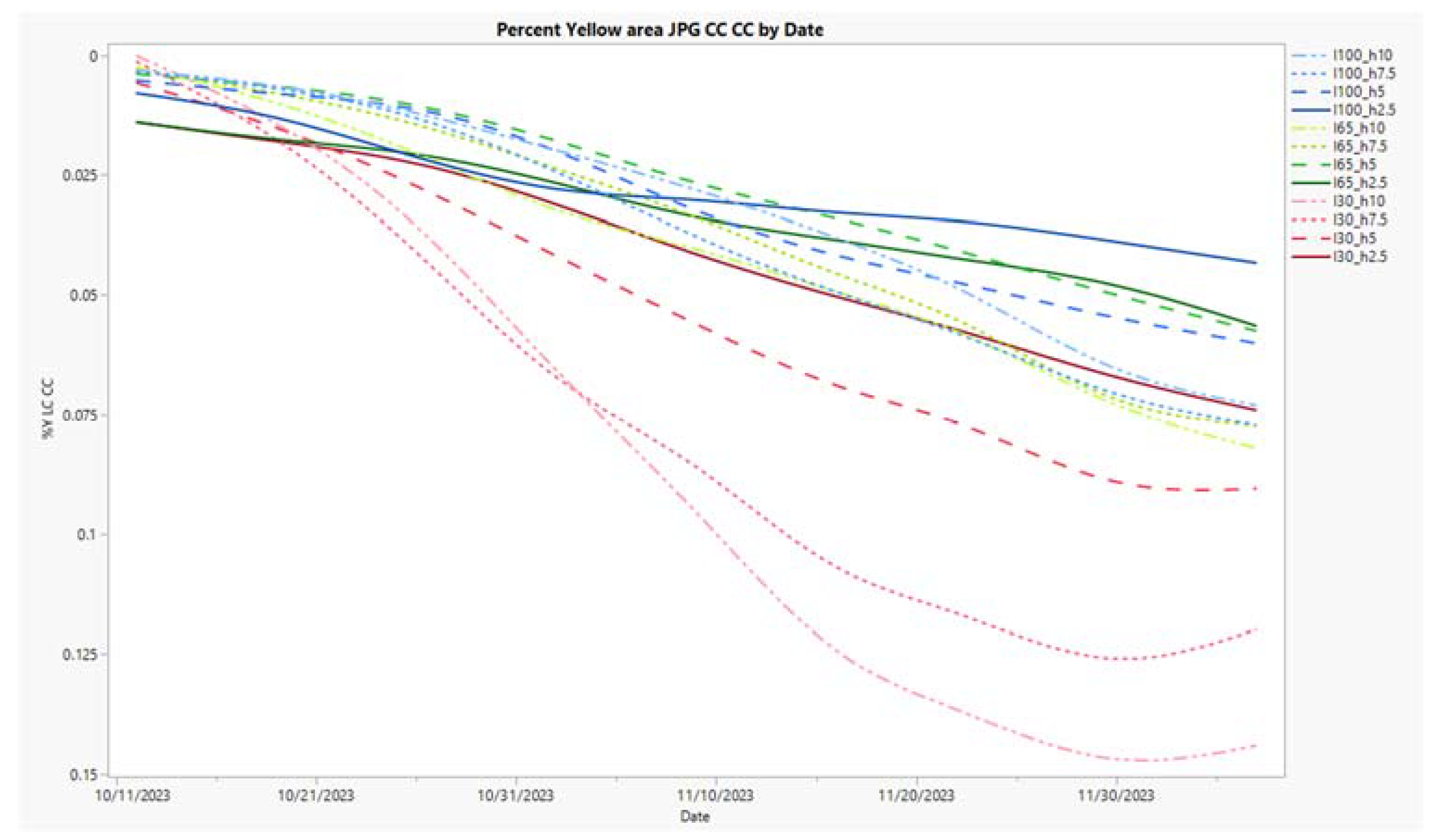
Figure 5. COMB2 time series chart where the combination term is plotted on the Y-axis and date is on the X-axis. The experimental treatments are labeled by their percentage of consumptive demand-based irrigation supplied (i = 100, 65, & 30 actual evapotranspiration replacement) and their mowing heights (h = 10, 7.5, 5.0, & 2.5 cm). Each treatment is grouped by irrigation level and uniquely colored, the line pattern is based on mowing height. Results show reduced change over time, but increased treatment separation when compared to NDVI and %Y (Figure 3 and Figure 4).

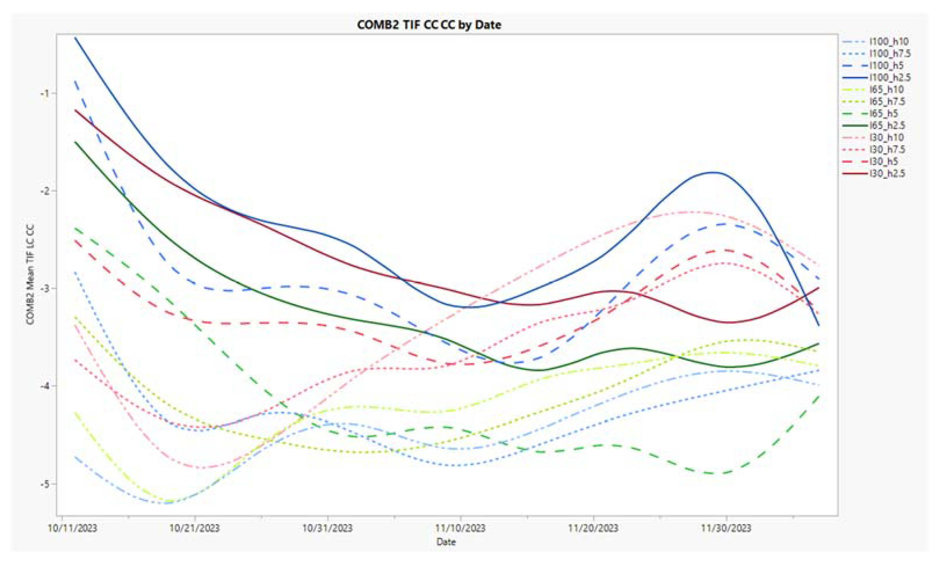
Table 1. Color classification segmentation pixel value ranges used in the Python process, where Hue is scaled 1 to 180 and Saturation and Value are scaled 0 to 255 for fractional living plant cover, yellow and green as %C, %Y and %G respectively.

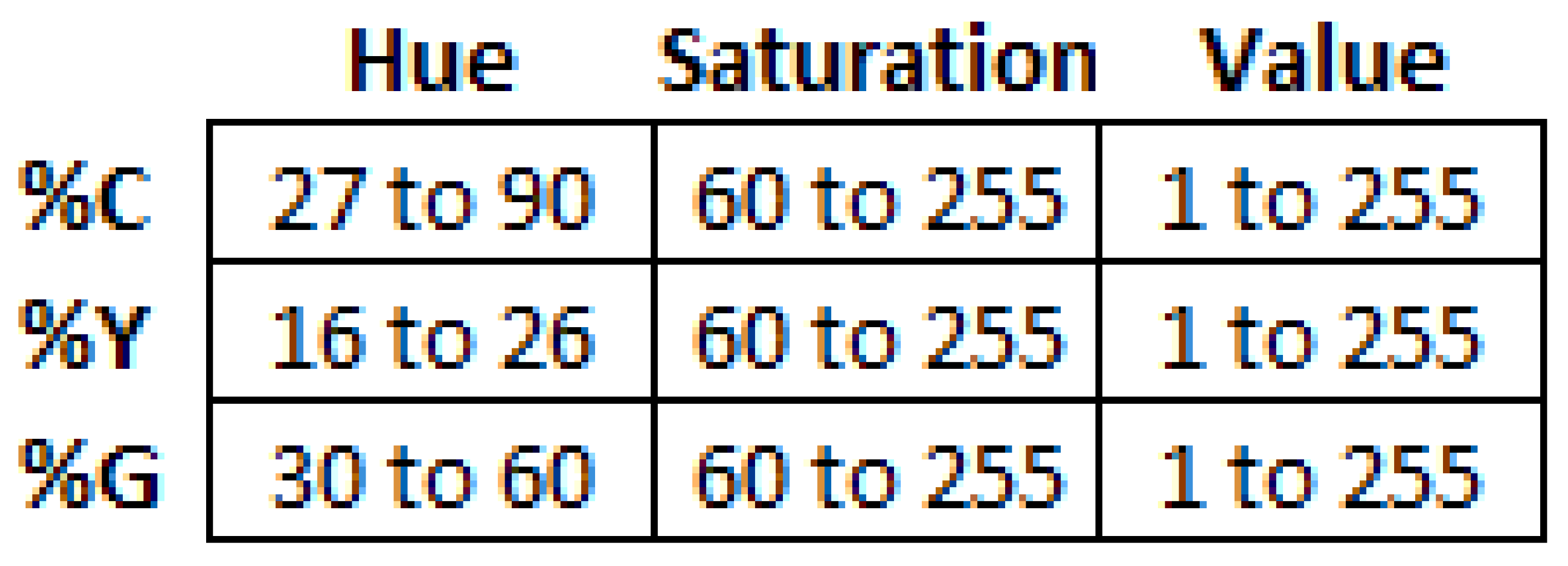
Table 2. Person’s correlation coefficient (R) and Coefficient of determination (R²) values for image metrics and associated reference measurements. The number of observations is noted in parenthesis beside the reference measurement in the top row. The file format and corrections applied are listed in the left column for each image metric. Bold font identifies which file format and correction had the highest correlation with a reference measurement.

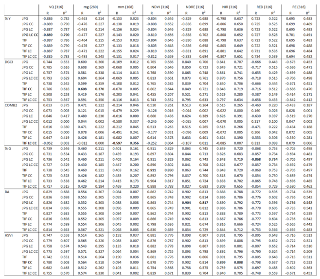
Table 4. Partial eta-squared (ηp2) effect sizes and significance level of permutational multivariate ANOVA results using 100,000 iterations, for the experimental treatments mow height (Mowing or M), water supplied (Irrigation or I) and date of measurement (Date or D), with interactions, on VQ, NDVI, and image metrics. The file format and image correction applied are noted above the variable name. ηp2 values indicate percentage of variance accounted by the effects. Significant difference for means is indicated as, not significant, p ≤ 0.05, p ≤ 0.01, and p ≤ 0.001, by symbols, NS, *, **, and *** respectively.

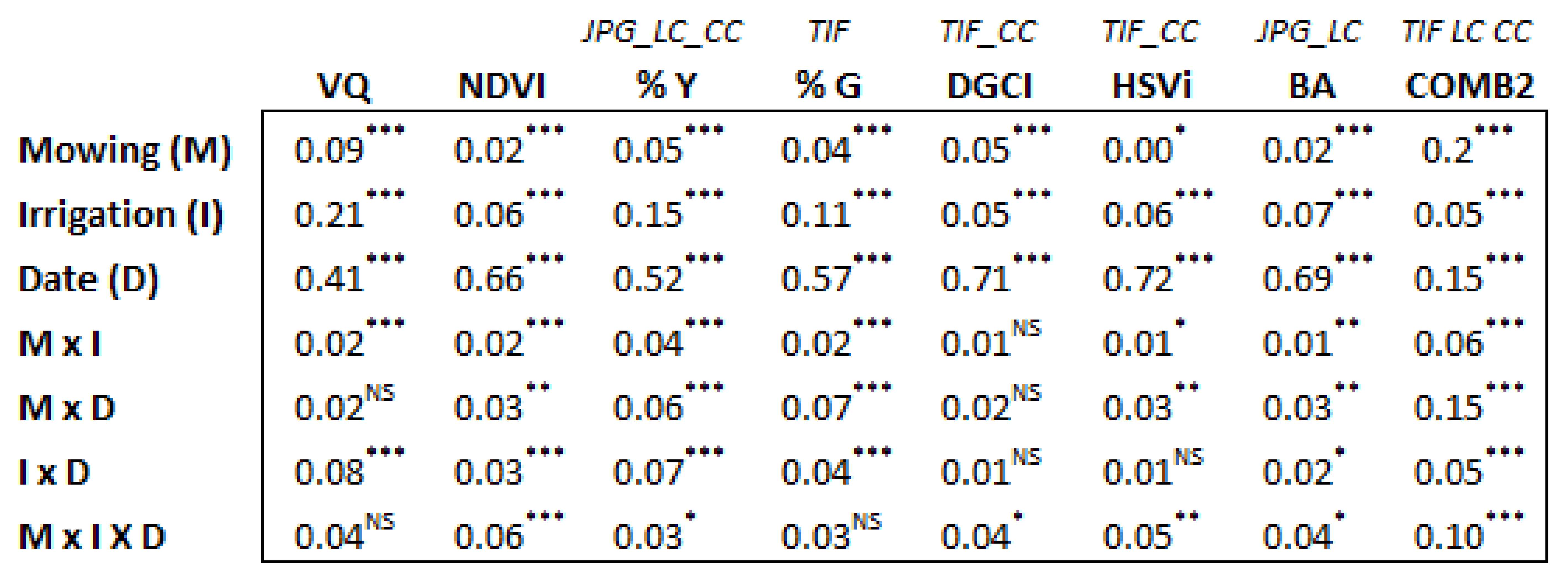
Disclaimer/Publisher’s Note: The statements, opinions and data contained in all publications are solely those of the individual author(s) and contributor(s) and not of MDPI and/or the editor(s). MDPI and/or the editor(s) disclaim responsibility for any injury to people or property resulting from any ideas, methods, instructions or products referred to in the content.

© 2024 by the authors. Licensee MDPI, Basel, Switzerland. This article is an open access article distributed under the terms and conditions of the Creative Commons Attribution (CC BY) license (http://creativecommons.org/licenses/by/4.0/).

Copyright: This open access article is published under a Creative Commons CC BY 4.0 license, which permit the free download, distribution, and reuse, provided that the author and preprint are cited in any reuse.

Downloads

148

Views

Comments

Subscription

Notify me about updates to this article or when a peer-reviewed version is published.

MDPI Initiatives

Important Links

Choose an area of interest and we will send you notifications of new preprints at your preferred frequency.

Disclaimer