Determination of Local Heat Transfer Coefficients and Friction Factors at Variable Temperature and Velocity Boundary Conditions for Complex Flows

Preprint

Article

Determination of Local Heat Transfer Coefficients and Friction Factors at Variable Temperature and Velocity Boundary Conditions for Complex Flows

Altmetrics

Downloads

105

Views

Comments

A peer-reviewed article of this preprint also exists.

Christopher Hartmann^*

Jens von Wolfersdorf

Christopher Hartmann^*

Jens von Wolfersdorf

This version is not peer-reviewed

Submitted:

14 August 2024

Posted:

14 August 2024

You are already at the latest version

Alerts

Abstract

Transient conjugate heat transfer measurements under varying temperature and velocity inlet boundary conditions at incompressible flow conditions were performed for flat plate and ribbed channel geometries. Therefrom local adiabatic wall temperatures and heat transfer coefficients are determined. Those data are analyzed using typical heat transfer correlations, e.g. Nu=CRe^mPr^n determining the local distribution of C and m. It is shown that they are closely linked. A relationship lnC=A−mB is observed with A and B as modeling parameters. They could be related to parameters in log law or power law representations for turbulent boundary layer flows. The parameter m is shown to have a close link to local pressure gradients and therewith near wall streamlines as well as friction factor distributions. A normalization of the C parameter allows to derive a Reynolds analogy factor and therefrom local wall shear stresses.

Keywords:

Subject: Engineering - Aerospace Engineering

1. Introduction

The accurate determination of wall shear stresses during flight missions plays a crucial role in the analysis and optimization of aircraft structures and in ensuring safety and efficiency in the aviation industry. In addition, the thermal load on the engine components during a typical flight mission with different operating points and transient effects must also be taken into account for an optimal design. Conjugate heat transfer effects, as first formulated by Perelman [1], play a decisive role in this consideration. Hartmann et al. [2] showed that slow, transient processes can be modeled very well with a quasi-stationary approach, even for complex flow structures. Nevertheless lead strong changes in temperature and flow velocities to strong local changes in the heat transfer coefficients depending on the thermal boundary conditions (see Liu et al. [3]). The temporal changes in flow temperatures near the wall are of immense importance. According to Esfahani and Jafarian [4], for low velocities the thermal component of entropy generation dominates over the frictional component in the boundary layer and has a large contribution to it, especially at the wall. This leads to changes in the local dissipation. Moffat [5] stated, that for the determination of a reliable heat transfer coefficient the adiabatic wall temperature should be used as the reference temperature in order to be able to take these effects into account. This theoretical temperature, which is formed as a result of dissipation in a flow around a heat-impermeable, i.e. adiabatic, body, is different from the ambient temperature, which is often used as a reference temperature [6]. The present transient, conjugate experimental setup uses infrared thermography and an evaluation methodology according to Estorf [7] to obtain temporally and spatially resolved temperature and heat flux data, which take lateral heat conduction into account. This formal overdetermination of the boundary conditions, wall temperature and wall heat flux, at the interface is used to derive a method for determining adiabatic wall temperatures and adiabatic heat transfer coefficients under time-varying boundary conditions. The wall temperature information has then be used to estimate wall shear stresses, assuming Reynolds similarity for the range of investigated Reynolds numbers of the flow.

In this work a method to determine adiabatic wall temperatures and heat transfer coefficients for constant inlet temperature and velocity boundary conditions is extended for variable boundary conditions. Subsequently, a simple correlation between heat transfer and friction factor from the model presented, is applied. This is compared with known correlations from the literature and then analyzed with regard to the physical significance of its parameters. Furthermore, the derived model is applied to more complex geometries and a method to determine temporal and spatial wall shear stress distributions only by measuring wall temperatures is shown.

2. Experimental Setup

The experimental test facility for local time-resolved transient heat transfer measurements has been designed by Liu et al. [8]. Brack et al. [9] modified the basic setup to investigate unsteady convective heat transfer under controlled airflow velocity and temperature variation and Hartmann et al. [2] adapted it to measure time-resolved transient heat transfer phenomena for different materials under various operating conditions. The experimental setup is shown in Figure 1.

Air is sucked by a vacuum pump from the ambient through a dust filter, heated up by a mesh heater entering the test section with a constant cross section of

0.12 m \times 0.15 m

. The time-variable temperature and velocity at the inlet of the channel can be set independently using a LabVIEW routine (see Brack et al. [9]). Two hot-wire anemometers from SVMtec monitor the inlet boundary conditions, measuring the inlet temperature (CCT) and the inlet velocity (CTA). Both are located

0.205 m

upstream the flat plate. The in the center of the channel positioned plate has the dimensions

0.92 m \times 0.12 m \times 0.03 m

, dividing the test section into two sub-channels with an aspect ratio of

2 : 1

. The plate is made from perspex with the possibility to change an inlay with the dimensions

0.25 m \times 0.06 m \times 0.015 m

visualized in Figure 2a. For the results presented here, quartz is chosen as second material. In addition to this geometry, a plate with five V-shaped ribs is also investigated, as shown in Figure 2b. The

90^{\circ}

squared ribs with a pitch of

p = 0.1 m

and dimensions of

e = 10

, are glued onto test plate, resulting in two visible ribs within the field of view (FOV).

At the beginning of the flat plate a trip wire ensures a turbulent flow. The optical access for the IRT camera, a FLIR SC7600, is assured by a 5 mm thick

{CaF}_{2}

-window on the top of the test section. To maintain a consistent and uniform emittance, the test plate was coated with black paint type SPB100 from Hallcrest. For on-site calibration of the infrared thermography data, two surface thermocouples were embedded into the plate to measure its surface temperature.

Figure 3 shows the nine test cases examined. These are a nearly temperature jump (Jump), a temperature (Ramp A) or velocity ramp (Ramp B), pulsations in temperature (Pulsation A) and temperature and velocity (Pulsation B) as well as four transient cycles (Cycle A-D).

The boundary conditions

T_{f}

and

u_{f}

were measured with a frequency of 4000 Hz by the two hot-wire anemometers at the channel inlet. The wall temperature

T_{w}

was temporally and spatially resolved with a frequency of 25 Hz and a spatial resolution of

0.4 mm / pixel

for

t = 150 s

using the IRT-camera, who measures the surface radiation in a spectral range from

1.5 μ m

5.1 μ m

. To avoid undesirable interference, the data were filtered by means of a 3D gaussian filter. For a better data handling the frequency for all measurements was afterwards reduced to 5 Hz, which does not affect the quality of the results (cf. Hartmann et al. [2]). The wall heat flux

{\dot{q}}_{w}

was temporally and spatially resolved, by a method according to Estorf [7], which is based on the analytical solution of the transient heat transfer equation within the wall for constant material properties and ensures the equality of the heat flux into the solid and of the fluid. The method requires isothermal initial conditions and semi-infinite wall assumption. With

T_{w}

{\dot{q}}_{w}

and the inlet temperature as reference temperature of the fluid

(T_{ref} = T_{f})

, the wall heat transfer coefficient

h_{w}

can be calculated using Newton’s law of cooling:

h_{w} = \frac{{\dot{q}}_{w}}{T_{w} - T_{ref}}

(1)

or using the adiabatic wall temperature

T_{aw}

as proposed by Moffat [5]

h_{aw} = \frac{{\dot{q}}_{w}}{T_{w} - T_{aw}} .

(2)

The measured quantity

T_{f}

u_{f}

T_{w}

as well as the evaluated ones,

{\dot{q}}_{w}

and

h_{w}

are subject to uncertainties. Based on the method of Moffat [10] the relative uncertainties for

δ {\dot{q}}_{w} / \dot{q}

and

δ h_{w} / h_{w}

vary between

10 %

and

15 %

depending on the mission, evaluation position and time (see Brack et al. [9] or Hartmann et al. [2] for details).

3. Results

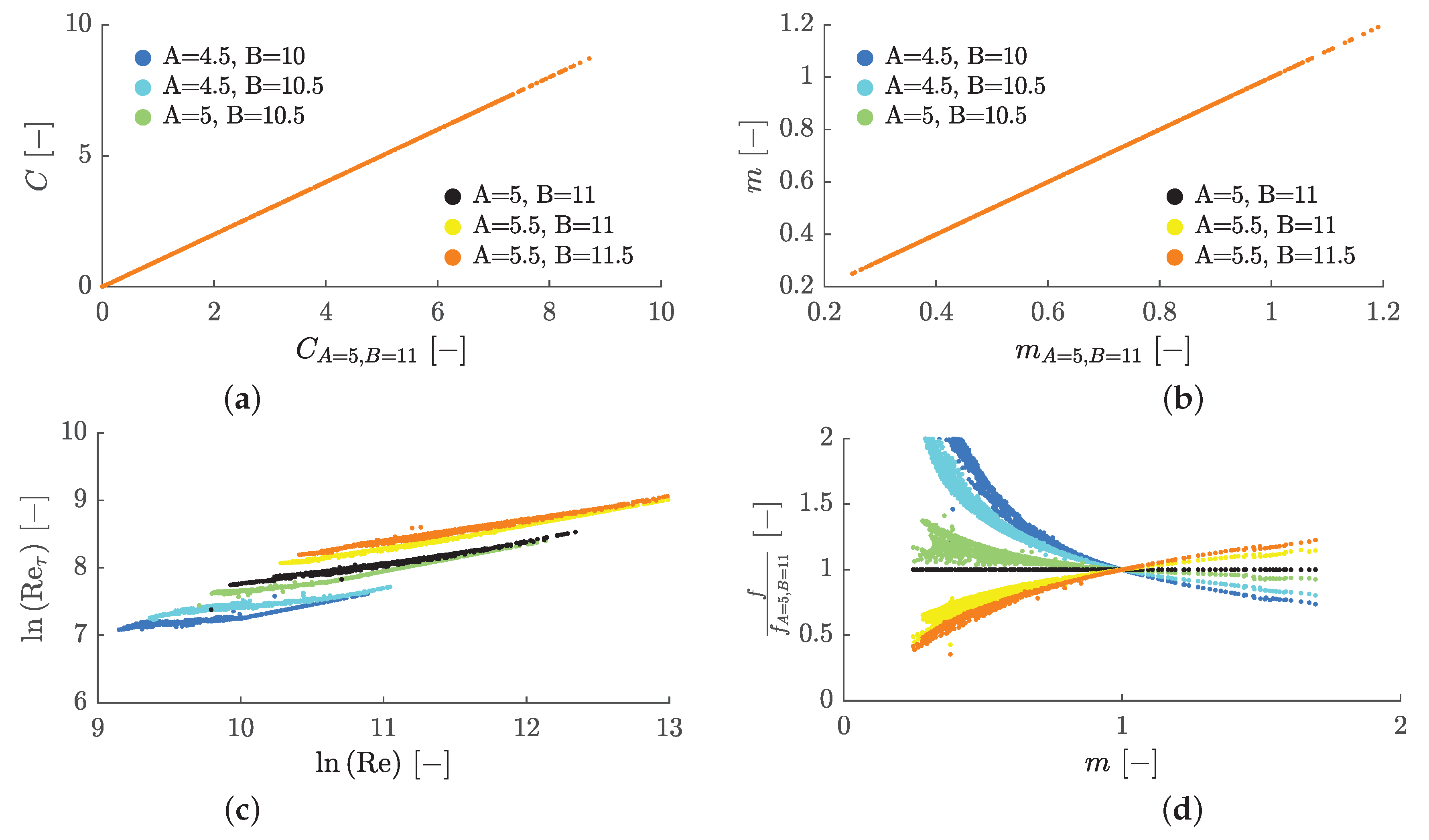
First, a method for determining adiabatic wall temperatures under arbitrary flow and temperature boundary conditions is derived. The parameters found are then interpreted for the case of the flat plate and a relationship to calculate friction factors is introduced. Finally, the method is applied to more complex flow situations.

Method for Determining Adiabatic Wall Temperatures

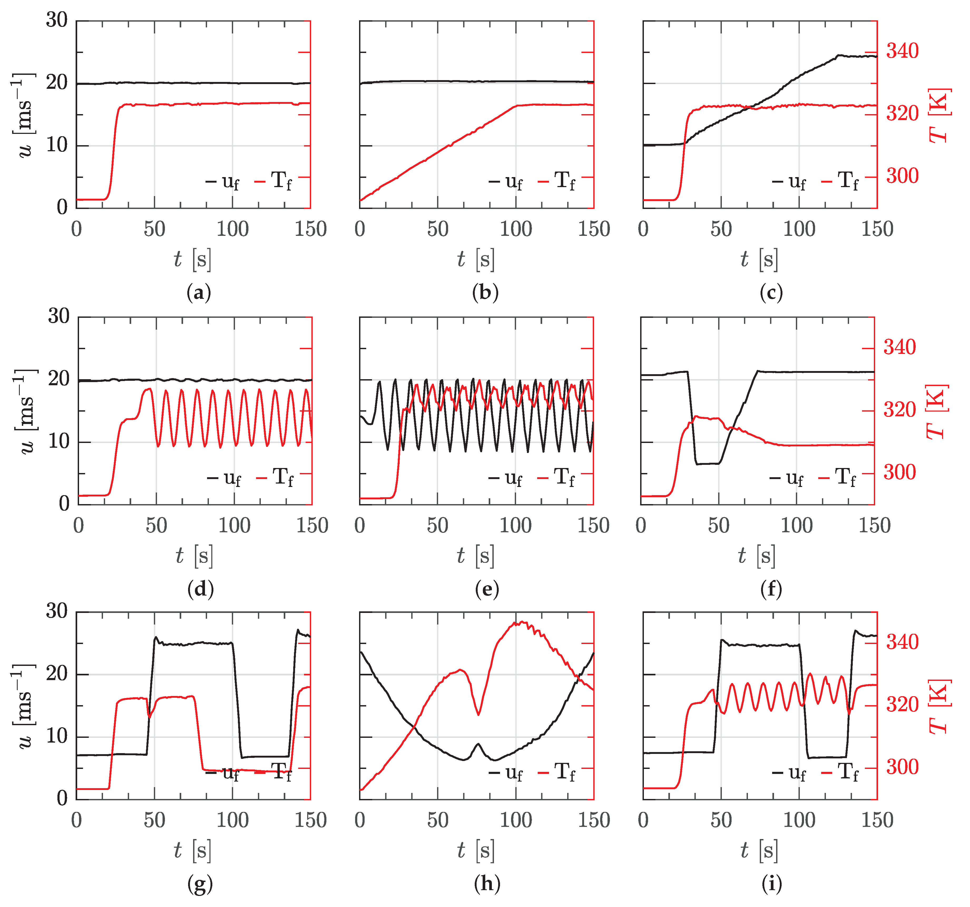
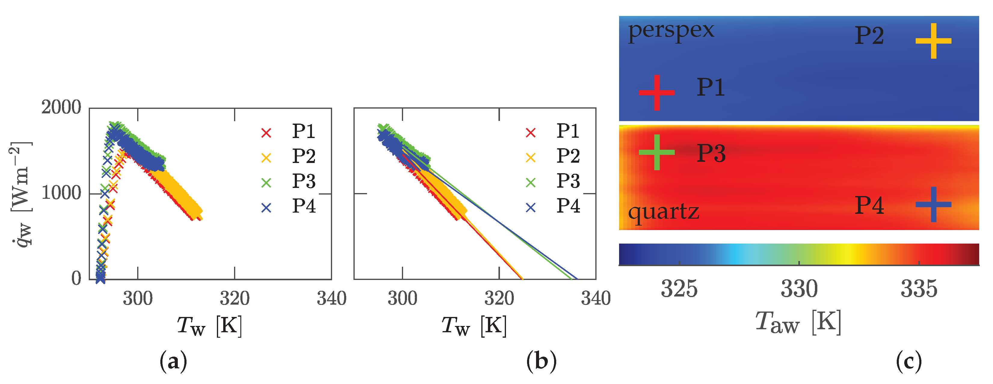
A widely used method for determining adiabatic wall temperatures at constant inlet temperatures and velocities is the adiabatic method according to Goldstein et al. [11] as a special case of the isotherm method according to Eckert [12]. Since both, the wall temperature as a measured variable and the wall heat flux, are known in the present study with spatial and temporal resolution, they can be plotted against each other for the Jump test case with a constant inlet temperature of

T_{f} = 323.15 K

(cf. Figure 3a) for selected pixels (see Figure 4) for perspex or quartz, respectively.

Here, the resulting curve first rises at the moment of the temperature jump (see Figure 3a), reaches its maximum there and then falls linearly. To determine the adiabatic wall temperature, a regression line of degree unity is drawn through the linear part - all time points greater than

t > 30 s

in Figure 4b. By extrapolating the straight line to the point of intersection with the abscissa at

{\dot{q}}_{w} = 0 \frac{W}{m K}

, the adiabatic wall temperature is obtained. The negative slope of the extrapolation line corresponds to the constant, adiabatic heat transfer coefficient. If the method is applied to all pixels in the field, a variation of the adiabatic wall temperature between

T_{aw} = 323 K . . . 327 K

can be seen in Figure 4c for perspex or between

T_{aw} = 333 K . . . 337 K

for quartz, respectively. The higher resulting adiabatic wall temperatures for quartz result from the effect, that quartz heats up much faster compared to perspex. According to Esfahani and Jafarian [4], the lower temperature differences at constant fluid temperature and fluid velocity lead to a comparatively increased entropy generation.

To take dissipation effects into account, a coefficient

β

is introduced. Based on Bacci et al. [13], this is defined as the ratio of the difference between the adiabatic wall temperature

T_{aw}

and the start/ambient temperature of the experiment

T_{0}

to the fluid temperature

T_{f}

and

T_{0}

β = \frac{T_{aw} (t) - T_{w} (t = 0)}{T_{f} (t) - T_{w} (t = 0)} = \frac{T_{aw} (t) - T_{0}}{T_{f} (t) - T_{0}} .

(3)

For a value of

β = 1

, the fluid temperature and adiabatic wall temperature coincide. At this point,

β

formally is a time-depending variable. However, for simplicity,

β

is assumed as a time-invariant variable similar to Bacci et al. [13]. Inserting

β

into Newton’s law of cooling (Equation 2) results in:

{\dot{q}}_{w} = h_{aw} \cdot β (T_{f} - T_{0}) - h_{aw} (T_{w} - T_{0}) .

(4)

This corresponds to the mathematical form of a slope-intercept form of a plane with the abscissa

T_{f} - T_{0}

, the ordinate

T_{w} - T_{0}

and the applicate

{\dot{q}}_{w}

. Thus, analogous to the regression line at constant inlet velocity, a regression plane can be calculated for a time-varying fluid temperature at constant inlet velocity. This is exemplified in Figure 5 by the test cases Pulsation A, Ramp A and Jump, for point P1 (cf. Figure 4c) and for perspex.

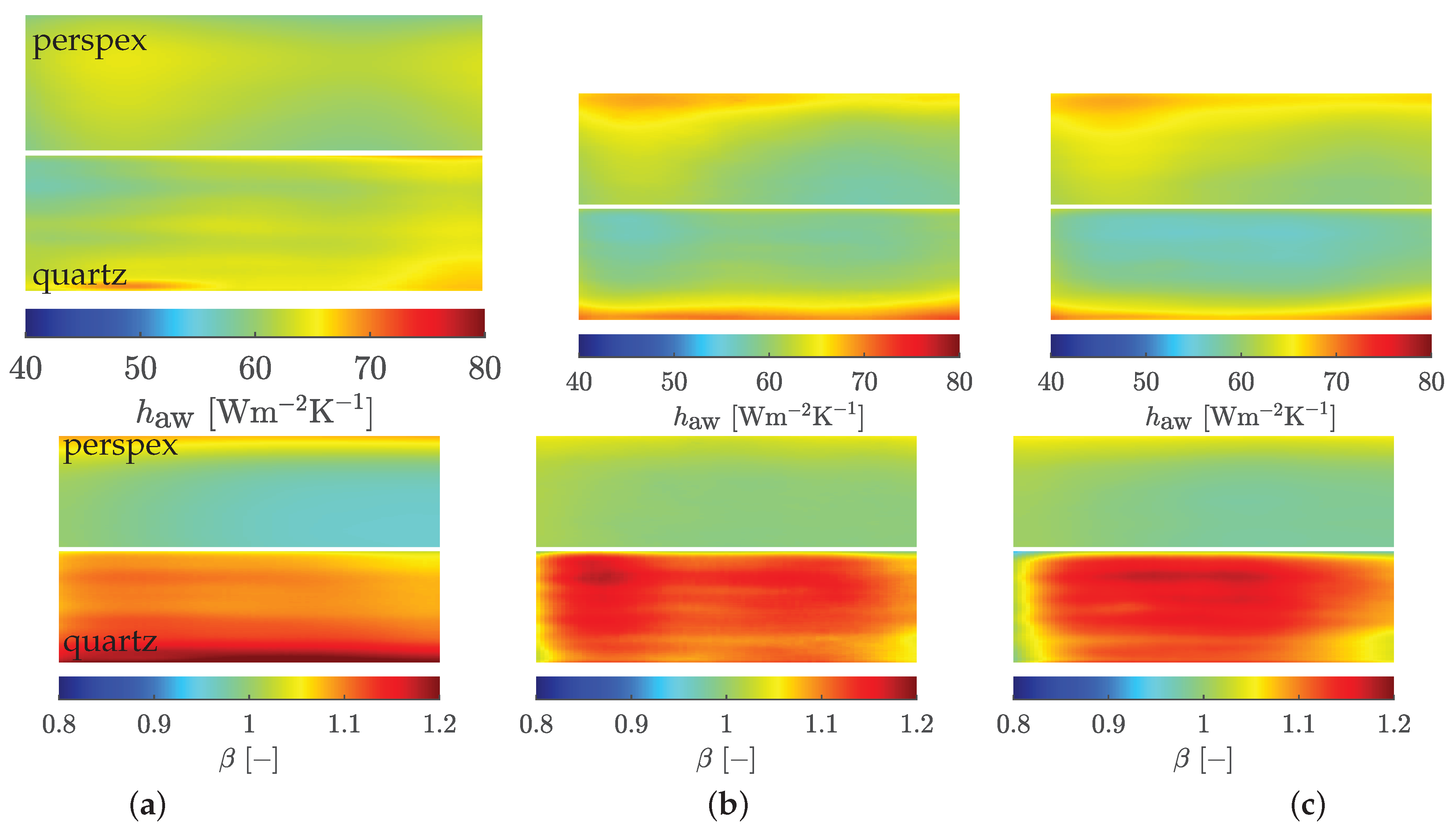
For a time-varying inlet temperature at constant velocity, the adiabatic heat transfer coefficient should be constant. This can be seen comparing the resulting adiabatic heat transfer coefficient from the three test cases with approximately equal fluid velocity

u_{f} \approx 20 m s^{- 1}

in Figure 6. For both materials, perspex and quartz, the adiabatic heat transfer coefficient is fairly constant at

h_{aw} \approx 60 W m^{- 2} K^{- 1}

(cf. Hartmann et al. [2]). Due to the temperature pulsation and the complex control of the inlet velocity, which varied slightly for Pulsation A (see Figure 3d), the heat transfer coefficient

h_{aw}

also varies barely (cf. Figure 6a). For more constant velocity courses at Ramp A (Figure 6b) and Jump (Figure 6c), there are hardly any differences. Furthermore, the somewhat increased values towards the channel side walls, related to corner vortices of a channel flow (see Vinuesa et al. [14]) are visible. The bottom line in Figure 6 shows the resulting dissipation coefficients

β

. Due to the rapid heating and to assure

h_{aw}

being approximately constant,

β

is higher for quartz than for perspex. However, it hardly varies for the same material on different test cases.

To take time-depending fluid velocities into account, a quasi-steady model of the form

Nu (t) = C Re {(t)}^{m} \Pr {(t)}^{n}

(5)

is introduced based on typical heat transfer correlations (cf. Kays et al. [15]). Hereby, the Nusselt number as dimensionless temperature gradient on the wall is defined as

Nu = \frac{h_{aw} L}{k} .

(6)

L = 0.03 m

is half the channel height of the sub-channel under consideration. The thermal conductivity k is modeled temperature-dependent using the formula presented by Sutherland [16] with the coefficients according to White [17] at the corrseponding wall temperature

T_{w}

. The same is true for the dynamic viscosity

η

. This results in the Reynolds number defined as

Re = \frac{u_{f} L ρ_{f}}{η},

(7)

where

ρ_{f}

is calculated from the ideal gas equation. The coupling of the temperature with the velocity field is represented by the Prandtl number, which yields with constant specific heat capacity

c_{p} = 1004.4 \frac{J}{k g K}

\Pr = \frac{η c_{p}}{λ} .

(8)

The Prandtl number is often also regarded as the ratio of velocity to temperature boundary layer. The Prandtl exponent n depends on the thermal boundary condition. Acording to Hetsroni et al. [18],

n = 1 / 2

corresponds to a constant wall heat flux and

n = 1 / 3

to a constant wall temperature boundary condition, what was selected for the presented study. With the definitions of the dimensionless variables

Nu

Re

\Pr

from Equations 6-8, it yields

{\dot{q}}_{w} (t) = C \cdot Re {(t)}^{m} \cdot \Pr {(t)}^{1 / 3} \cdot \frac{λ (t)}{L} (β (T_{f} (t) - T_{w} (t = 0)) - (T_{w} (t) - T_{w} (t = 0))) .

(9)

Hartmann et al. [2] showed that the slow transient experiments studied here can be regarded as quasi-stationary, i. e. each point in time might be regarded as a stationary experiment of its own. Assuming Reynolds similarity for the flow in the investigated velocity range from

u_{f} = 5 m s^{- 1} . . . 25 m s^{- 1}

, this results in a total of

5200

data tuples

(T_{f}, u_{f}, T_{w}, T_{0}, {\dot{q}}_{w})

for the eight considered experiments (cf. Figure 3a-h), neglecting the first

20 s

of each experiment, because of the initial isothermal situation. To calculate the unknowns, the overdetermined system of equations is solved at each pixel. This is done using a nonlinear least-squares algorithm, the trust-region-reflective algorithm, as a subspace trust-region method based on the interior-reflective Newton method described in [19,20,21]. The optimized values for C, m and

β

are shown in Figure 7 for perspex or quartz, respectively.

C and m are relatively constant over the entire surface and

β

shows a similar distribution as in Figure 6 using Equation 4. Slight differences are visible between the two materials, resulting from the approximated choice of

β

. However, it is noticeable that C and m interact with each other. For example, C is slightly larger for quartz than for perspex, while m is slightly smaller.

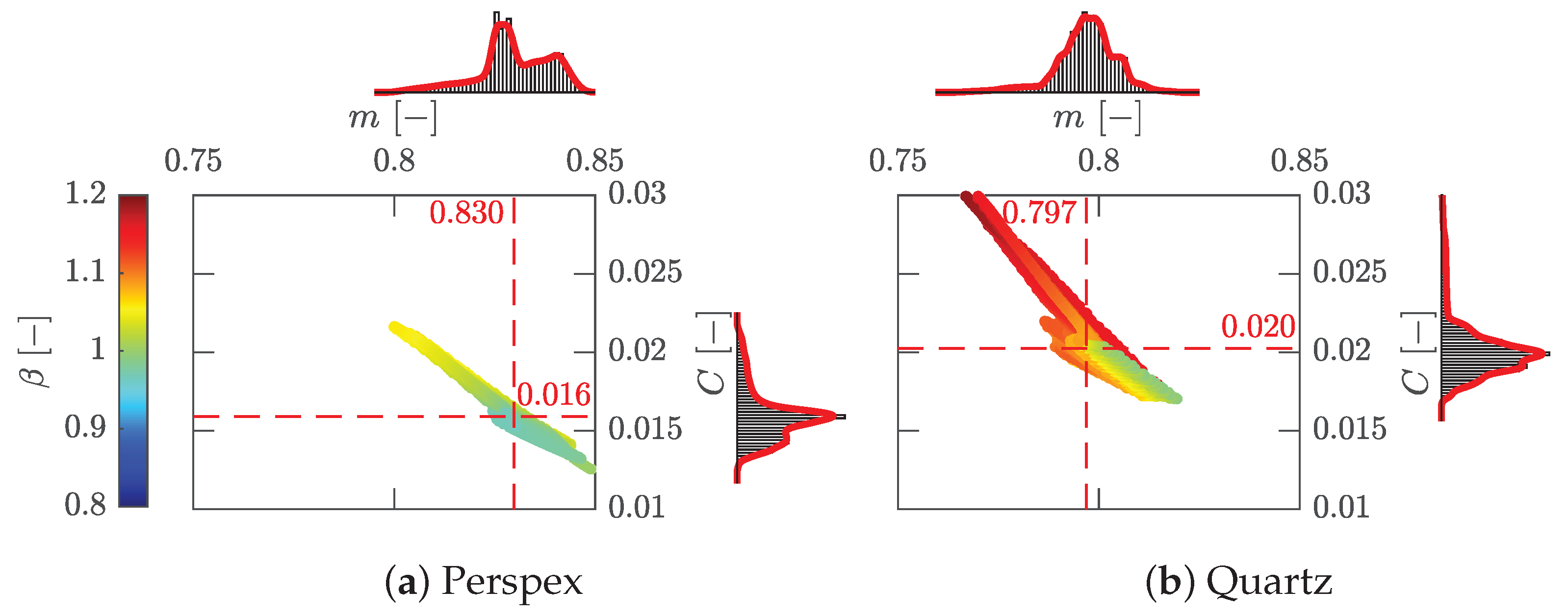
This becomes visible plotting C over m locally and adding

β

as color information as shown in Figure 8, where also the histograms of the optimized variables C and m as well as their statistical mean value are shown. The range of

C = 0.015 . . . 0.025

and

m = 0.75 . . . 0.85

correspond to typical values for turbulent channel or pipe flow correlations.

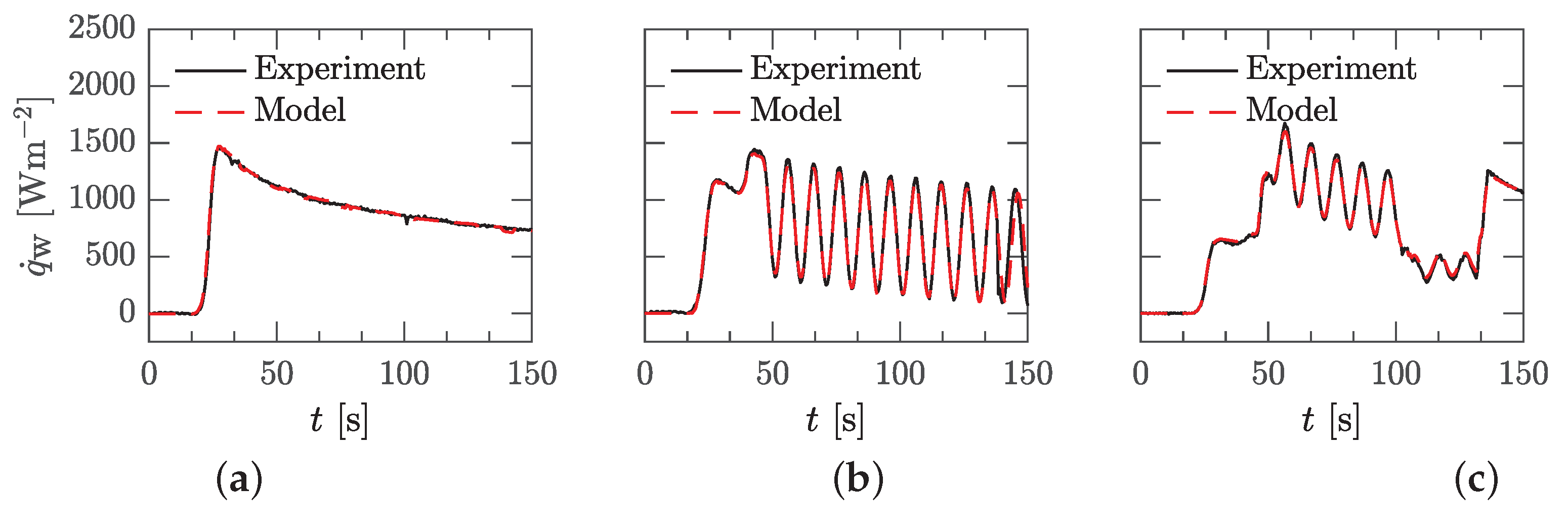
To evaluate the quality of the model, in Figure 9 the recalculated heat flux over time for three cases at evaluation point P1 (

C = 0.0239

m = 0.7843

β = 0.9722

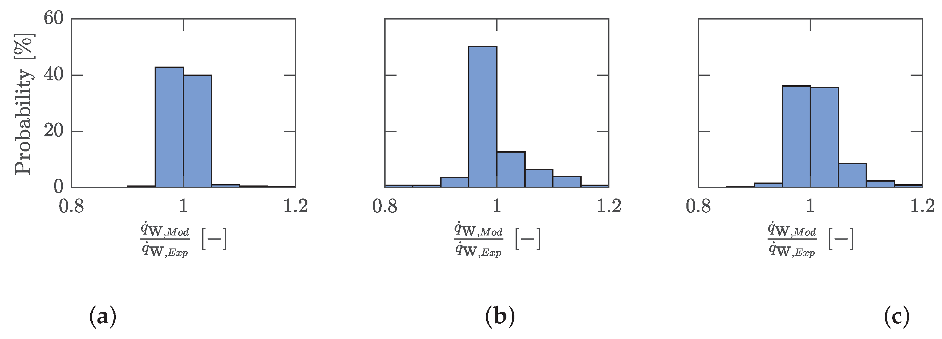
) is shown. Firstly, for the known cases of the Jump (cf. Figure 3a) and Pulsation A (cf. Figure 3d), which were part of the input data set. Secondly, for Cycle D (cf. Figure 3i), which was not part of the input data set, but was examined using the same experimental data evaluation and with highly non linear flow and temperature boundary conditions. The heat flux course over time is reproduced very well for all three test cases. In areas with strong gradients in the boundary conditions, the back-calculated curve is somewhat smoother, resulting from the optimization, which acts as a kind of filtering of all data. However, even the initial period without a temperature jump is reproduced very well. The deviations between the experimentally determined heat flux and the calculated one from the model are in agreement by

\pm 10 %

as can be seen in Figure 10, where all points in time are added in the histograms. Thus, a model could be derived which is able to reproduce the heat flux very well even for an unknown test case.

Flat Plate Flow

Figure 11 presents a composite diagram of the data from Figure 8a and Figure 8b. The logarithmic plot of C reveals a linear relationship between

ln (C)

and m, allowing the integration of perspex and quartz data into a single dataset. By incorporating the dissipation coefficient’s color information for both independently optimized parameters, a gradation according to

β

is observed. The slope of a resulting fitting line varies between

- 10.5

and

- 11.5

, with the offset ranging from

4.5

5.5

, depending on the data considered.

From Figure 11 with the new, also time-invariant, parameters A and B, it might be approximated:

ln (C) = A - m B .

(10)

In order to analyze the parameters A and B further, only perspex is considered. First, the basic approach from Equation 5 is evaluated. It is assumed that all heat fluxes are approximately dissipation corrected due to the introduction of

β

. Furthermore, the Prandtl number in the experiments is only weakly temperature dependent and will be regarded as a constant in the following. Logarithmizing and rearranging Equation 5 then yields:

ln (C) = ln (\frac{Nu}{\Pr^{1 / 3}}) - m \cdot ln (Re) .

(11)

A simple comparison of Equations 11 and 10 gives:

A = ln (\frac{Nu}{\Pr^{1 / 3}}), B = ln (Re) .

(12)

Interestingly, the same result is obtained if the approach from Equation 10 is used in Equation 5 and a functional equation is derived:

\frac{\partial Nu}{\partial m} = exp (A - m B) \cdot {Re}^{m} \cdot \Pr^{1 / 3} \cdot (ln (Re) - B) .

(13)

Setting this equation to zero, forms an envelope to the family of

Nu

Re

-curves (c.f. Afzal [22]) and substitute

exp (A - m B) \cdot {Re}^{m} \cdot \Pr^{1 / 3}

again by

Nu

yields:

\frac{\partial Nu}{\partial m} = Nu \cdot (ln (Re) - B) = 0 .

(14)

Since the Nusselt number can never be zero,

B = ln (Re)

. Formally, this representation is independent of the Prandtl number and its exponent n.

Insertion into the original model Equation 9 then results in an equivalent representation

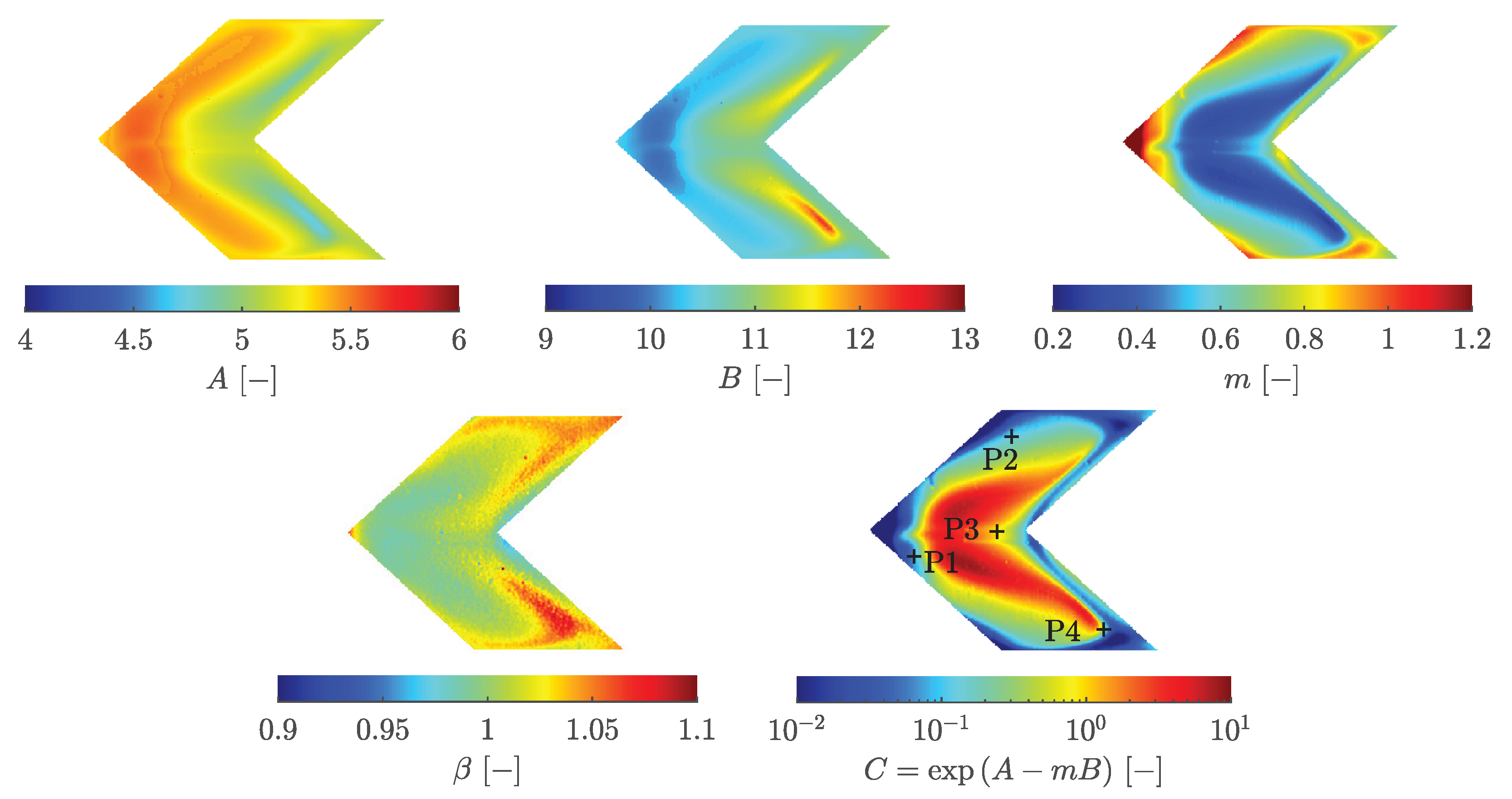
{\dot{q}}_{w} (t) = exp (A - m B) \cdot Re {(t)}^{m} \cdot \Pr {(t)}^{1 / 3} \cdot \frac{λ (t)}{L} (β (T_{f} (t) - T_{w} (t = 0)) - (T_{w} (t) - T_{w} (t = 0))) .

(15)

This gives a total of four parameters to optimize on the experimental data (A, B, m,

β

). Since C and m are considered as time-invariant variables, according to Equation 10, A and B are also considered time-invariant. Similar to

β

, both might be regarded as an effective Reynolds number

\bar{Re} = exp (B)

with a corresponding effective Nusselt number

\bar{Nu} = exp (A) \Pr^{1 / 3}

. The ratio is

\frac{Nu (t)}{\bar{Nu}} = {(\frac{Re (t)}{\bar{Re}})}^{m} .

(16)

In view of the the quasi-steady assumption,

Nu

and

Re

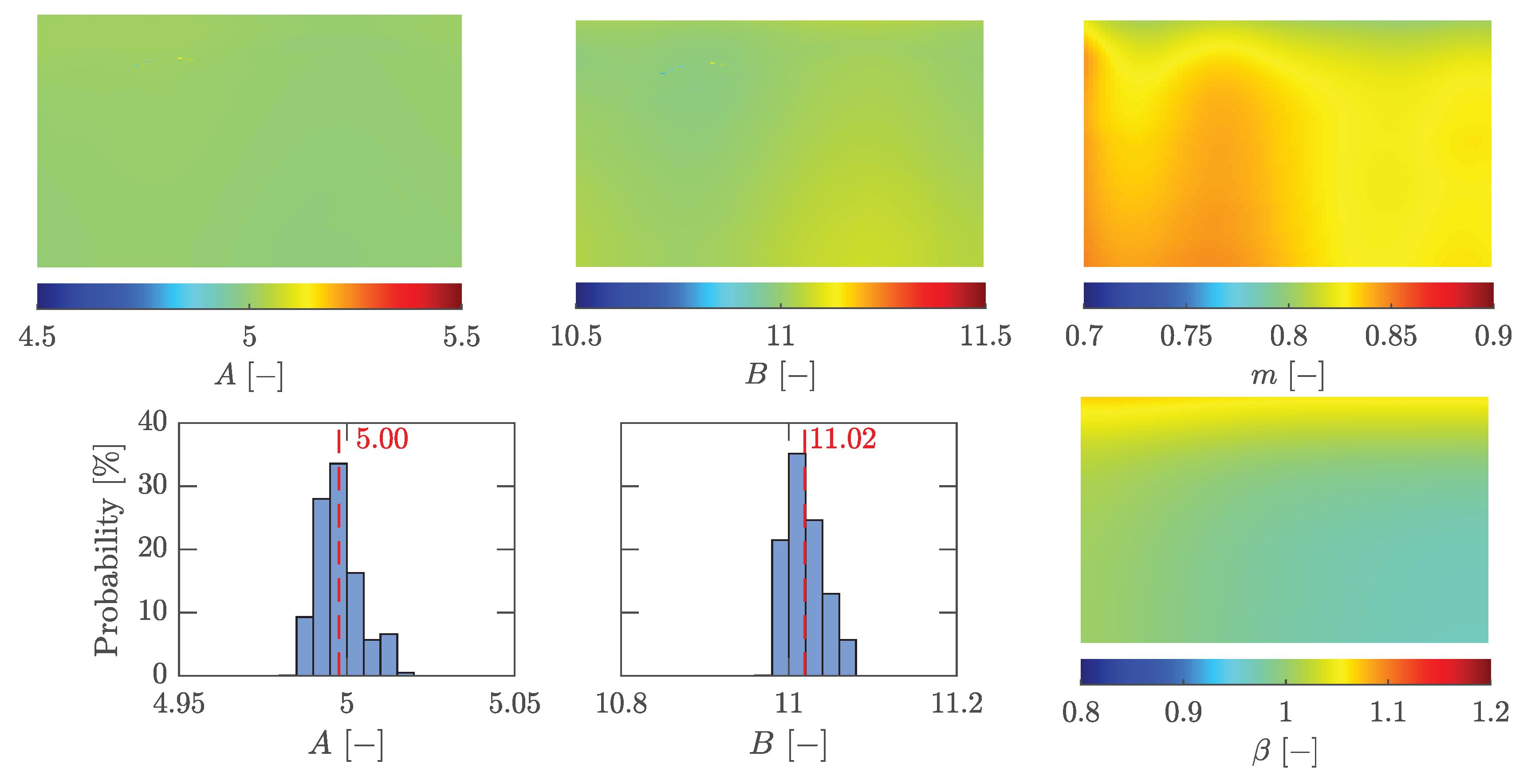
are treated as time-invariant parameters in the following. The results of the new optimization of Equation 15 can be seen in Figure 12. Due to the linear dependence of

ln (C)

on m, m itself and

β

remain unchanged, as expected. However, the optimization algorithm requires the specification of initial values. Since C now depends on A and B via Equation 10, there are an infinite number of equivalent combinations for A and B. Nevertheless, the initial values

A = 5

and

B = 11

as mean values of the observed range in Figure 11 are motivated by the fit of Equation 10 to the data for perspex and quartz. Thus, A and B show significantly less variation than C and are statistically distributed around the values

A \approx 5

and

B \approx 11

(cf. Figure 12).

With the values for

A = 5

and

B = 11

Nu = C {Re}^{m} \Pr^{1 / 3}

can also be written as

Nu = exp (5 - 11 m) {Re}^{m} \Pr^{1 / 3},

(17)

whereby C in Equation 5 becomes a function of m. With

m = 0.8

it yields

C = 0.0224

, what is similar to the known pre-factor and exponent of the Dittus-Boelter correlation, as introduced by McAdams [23,24]. By introducing the Stanton number,

St = \frac{Nu}{Re \Pr}

, in Equation 5 with Equation 10 it yields:

St \Pr^{2 / 3} = exp (A - m B) {Re}^{m - 1},

(18)

which reminds of the Colburn analogy

St \Pr^{2 / 3} = \frac{f}{2}

(cf. [25]) for the chosen Prandtl number dependency. Thus, the friction factor f can be written as

\frac{f}{2} = C {Re}^{m - 1} = exp (A - m B) {Re}^{m - 1} .

(19)

With the values for

A = 5

and

B = 11

from the optimization as well as with m between

0.75 . . . 0.85

, a comparison to known friction correlations can be made. With

m = 0.75

, this results in a pre-factor of

f = 2 exp (5 - 0.75 \cdot 11) = 0.0775

close to the correlation given by Blasius [26] with

{Re}^{- 0.25}

or for

m = 0.8

f = 0.0448

and

{Re}^{- 0.2}

close to the one given by Nikuradse [27]. The correlation of Blasius is only valid up to a Reynolds number of

R e < 10^{5}

and thereafter that of Nikuradse. It can therefore be concluded that both C and m are functions of the Reynolds number similar to the velocity profiles given by power law models (see Schlichting [6]). However, in the investigated Reynolds number range, C and m might be assumed to be constant as implied in Equation 9. Interestingly, going back to Equation 19 and using

B = ln (Re)

it yields

f = 2 exp (A - B),

(20)

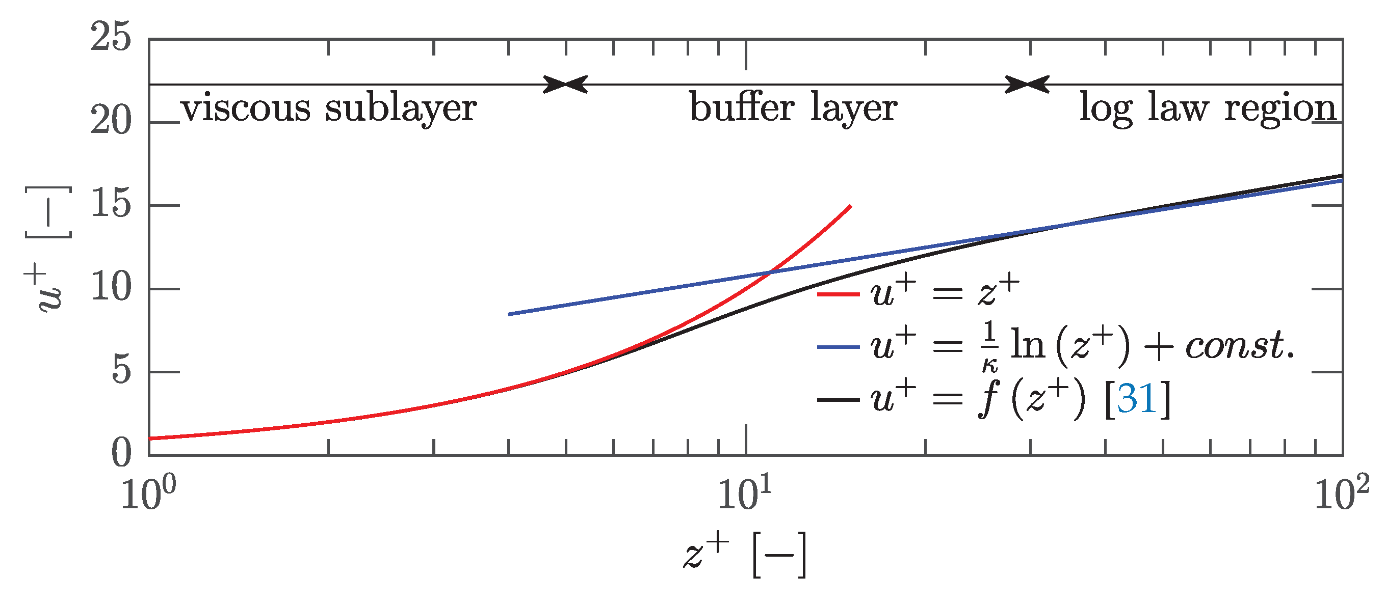
which does not depend on m any further. Friction factor relationships without a dependency on m were introduced, e.g. by Prandtl [28] in an implicit form for all Reynolds numbers derived from the log law. Classically, according to von Kármán [29], the viscous sublayer extends to

z^{+} = 5

, followed by a buffer zone and the logarithmic region. The mean velocity distribution within the viscous sublayer is obtained by

u^{+} = z^{+}

, whereas in the logarithmic region

u^{+} = \frac{1}{κ} ln (z^{+}) + c o n s t .

(21)

according to von Kármán [29] and Prandtl [28] is accepted. For turbulent flows with smooth walls the von Kármán constant of momentum transfer

κ

and the integration constant are specified in Coles [30] as

κ = 0.41

and

c o n s t . = 5.0

. Generalized functions for the velocity profile are given, e.g. by Reichardt [31] or Spalding [32]. In the equations to compare kinematic boundary layers, dimensionless velocities

u^{+} = \frac{u}{u_{τ}}, u_{f}^{+} = \frac{u_{f}}{u_{τ}}

(22)

are introduced, where the friction velocity

u_{τ} = \sqrt{\frac{τ_{w}}{ρ_{f}}}

(23)

is correlated with the wall shear stress

τ_{w} = η \frac{\partial u}{\partial z} |_{z = 0}

, which can be expressed in dimensionless form by:

\frac{f}{2} = \frac{τ_{w}}{ρ_{f} u_{f}^{2}} = \frac{1}{{u_{f}}^{+}^{2}} .

(24)

Introducing the dimensionless wall coordinate

z^{+} = \frac{z u_{τ}}{ν},

(25)

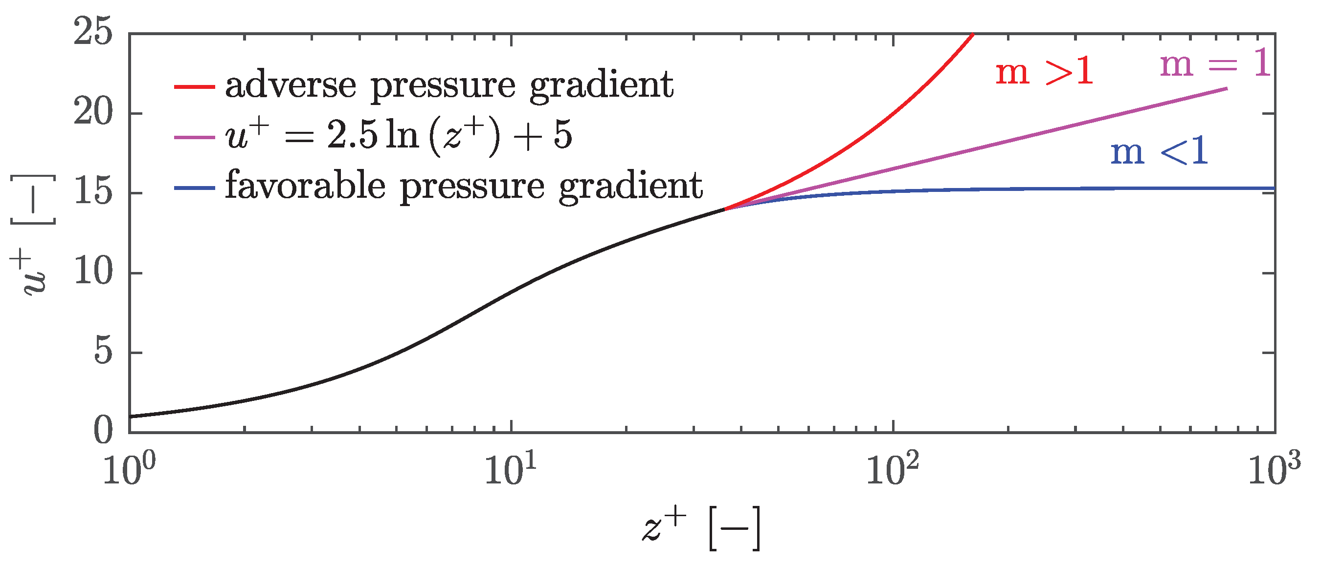
a characteristic velocity profile within the kinematic boundary layer is shown in Figure 13 assuming

κ = 0.4

and

c o n s t . = 5

The extrapolation of the inner law in the viscous sublayer

u^{+} = z^{+}

with the law of the wall at

z^{+} \approx 11 \approx B

, within the so-called buffer layer, gives

u^{+} = \frac{1}{κ} ln (u^{+}) + A .

(26)

Thus, A can be seen as the log law intercept and B would mark the match point between the extrapolated linear viscous sublayer and the logarithmic laws. At this point it holds [33]:

B = \frac{1}{κ} ln (B) + A .

(27)

Hence, B might be regarded as a measure of the sublayer thickness and will interact with the log law intercept A, and the von Kármán coefficient

κ

. All of them might vary with pressure gradient as described for example by Nickels [34], Nagib and Chauhan [35], Dixit and Ramesh [36] or Baxerres et al. [37]. From Equation 27,

κ

is given by

κ = \frac{ln (B)}{B - A} .

(28)

If B continues to represent a varying Reynolds number, according to Equation 27 for each B, there is an A representing the corresponding dimensionsless gradient at the wall. If

A = 5

and

B = 11

are set,

κ \approx 0.4

. Furthermore, inserting Equation 27 into Equation 20 yields

f = 2 exp (- \frac{1}{κ} ln (B)) = 2 exp (- \frac{1}{κ} ln (ln (Re)))

(29)

or equivalently,

N u = exp (- \frac{1}{κ} ln (ln (Re))) Re \Pr^{1 / 3},

(30)

which are explicit relationships describing friction factors and Nusselt numbers related to turbulent fully developed pipe or channel flow. Comparing Equations 29 and 30 in Figure 14 with correlations between Nusselt and Reynolds numbers or friction factors and Reynolds number in literature gives good agreement. Here, the derived relationships are compared with the friction correlations of Blasius1[26], Nikuradse2[27], Prandtl3 [28] and Petukhov4[38] or the Nusselt correlations of Dittus-Boelter5[23,24] and Kays et al. 6[15], respectively.

Furthermore, with

{Re}_{τ} = \frac{u_{τ} L}{ν} = Re \frac{1}{u_{f}^{+}} = Re \sqrt{\frac{f}{2}}

(31)

and Equation 20, it yields

{Re}_{τ} = exp (\frac{A + B}{2})

(32)

and

u_{f}^{+} = exp (\frac{B - A}{2}) .

(33)

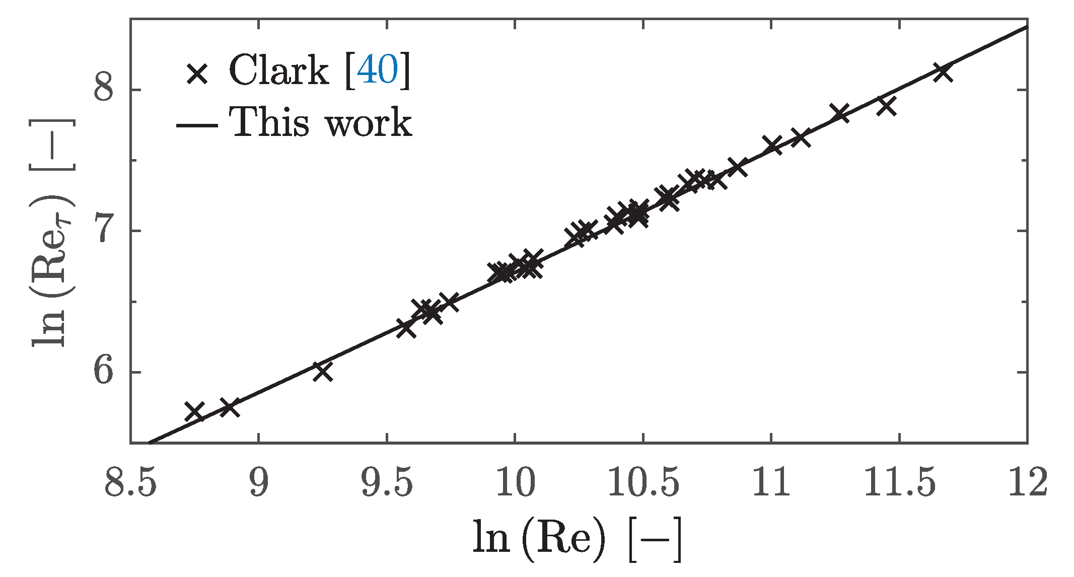
For turbulent channel flows Hussain and Reynolds [39] determined a range of

A = 4 . . . 6

and Clark [40] for

B = 8.5 . . . 12

, respectively. In Figure 15

ln ({Re}_{τ})

is plotted over

ln (Re)

. Interpreting B again as Reynolds number according to Equation 12, varying A with B according to Equation 27 and assuming

\frac{1}{κ} = 2.86

as used by Clark [40], it is possible to reproduce Clark’s data fairly well.

The relationship

ln (C) = A - m B

from Equation 10 is obtained from Blasius’ friction law [26]. Therefrom the velocity power law is derived as first shown by Prandtl [28] and taken up by Schlichting [6]. In general,

\frac{f}{2} = C {Re}^{m - 1} .

(34)

Thus, for the wall shear stress it yields:

τ_{w} = C {Re}^{m - 1} ρ u_{f}^{2} = ρ C u_{f}^{1 - m} ν^{1 - m} L^{m - 1} = ρ u_{τ}^{2} .

(35)

Rearranging gives:

C = \frac{{Re}_{τ}^{1 - m}}{{u_{f}}^{+}^{2 - 1 + m}} = \frac{{Re}_{τ}^{1 - m}}{{u_{f}}^{+}^{1 + m}}

(36)

with Equations 32 and 33 it yields

\begin{matrix} ln (C) & = (1 - m) ln ({Re}_{τ}) - (1 + m) ln (u_{f}^{+}) \\ = ln (\frac{{Re}_{τ}}{u_{f}^{+}}) - m ln ({Re}_{τ} u_{f}^{+}) = A - m B, \end{matrix}

(37)

showing the relationship between

ln (C)

and m with

u_{f}^{+}

and

{Re}_{τ}

. An alternative description of the velocity distribution in pipe or channel flows is the so-called power law

u^{+} = D z^{+^{α}} .

(38)

Schlichting [6] showed that the

α = \frac{1}{7}

is a good approximation to the log law Equation 21 for

Re < 10^{5}

, where the pre-factor D and the exponent

α

varying with the Reynolds number. Several relationships for the power law are given for example by Afzal et al. [41]. Barenblatt [42] specifies D and

α

as a function of the Reynolds number for pipe flows:

D = \frac{1}{\sqrt{3}} ln (Re) + 2.5 = \frac{\sqrt{3} + 5 α}{2 α}, α = \frac{3}{2 ln (Re)} .

(39)

Barenblatt et al. [43] stated this scaling law holds also for turbulent boundary layers if the Reynolds number is chosen appropriate. Using Barenblatt’s [42] relationship in Equation 39 between

α

and

Re

and again interpreting

exp (B)

as Reynolds number, it is possible by Equation 20 to reproduce his friction factors given by

f = \frac{2}{{(\frac{e^{\frac{3}{2}} (\sqrt{3} + 5 α)}{2^{α} α (1 + α) (2 + α)})}^{\frac{2}{1 + α}}} .

(40)

Furthermore, Barenblatt [42] gives a formulation for

{Re}_{τ}

depending on

α

{Re}_{τ} = {(\frac{e^{\frac{3}{2}} 2^{α} α (1 + α) (2 + α)}{(\sqrt{3} + 5 α)})}^{\frac{1}{1 + α}} .

(41)

Using this and additionally Equation 32 gives A, and with Equation 28 also

κ

depending on the Reynolds number only. For any Reynolds number, with the resulting parameters A and B,

κ \approx 0.4

is obtained. Barenblatt [42] showed that the resulting envelope of power-law curves matches a logarithmic law with

u^{+} = 2.5 ln (z^{+}) + 5.1

, see also e.g. Afzal et al. [44].

Furthermore, Barenblatt et al. [45] consider the intermediate region between the viscous sublayer and the external flow consisting of two self-similar structures described by power laws and separated by a sharp boundary. The inner region scaling law is assumed to be universal, whereas the outer scaling law depends on the pressure gradients. In fact, the match point determines a characteristic length for an effective Reynolds number, which lies within the range

ln (Re) = B = 9 . . . 13

for different experimental data (cf. [45]) and is according to Barenblatt et al. [46] related to the wall-region thickness for turbulent boundary layer flows. The parameters

A \approx 5

and

B \approx 11

found for the flat plate, were linked to the extrapolated interaction between the linear part,

u^{+} = z^{+}

, of the viscous sublayer and the log law in the buffer layer (cf. Wosnik et al. [47]). However, the presented observations might also be interpreted as the interaction of the two scaling laws proposed by Barenblatt et al. [45] in the intermediate or overlap region.

A similar interpretation of a parameter m - probably by incidence - as a measure for the thickness of the inner layer, which is still influenced by the wall was made by Szablewski [48] in his mixing length model, which he suggested as an outer region analogon to the model of van Driest in the buffer layer [49]. Therefore, m should be pressure gradient dependent similar as the van Driest damping length parameter (see e.g. Cebeci and Bradshaw [50]) and might be interpreted as an connecting parameter for so called quasi-equilibrium pressure-gradient boundary layers, see e.g. Baxerres et al. [37].

Complex Flow Situations

So far, only the experimental data for a flow over a flat plate have been considered. The pressure forces occurring here are moderate and the question arises how the model behaves with a more complex flow. For this purpose, a further geometry with five V-shaped ribs arranged one behind the other was investigated (cf. Figure 2b). First, Figure 16 shows the optimized values of Equation 9 with the initial values

C = 0.023

m = 0.8

and

β = 1

analogous to the optimization of the experimental data of the flat plate.

In contrast to the flat plate, there is a significantly larger variation in C and m.

β

remains in a similar range as for the flat plate geometry. This consistency is expected, as the temperature and velocity boundary conditions are unchanged, and the resulting wall temperatures for the individual test cases have not increased drastically (see Hartmann et al. [2]). However, the rib geometry induces additional vortices, evident in the distribution of C and m. In the core zone, the flow is strongly accelerated by the preceding rib, causing the m value to decrease significantly, reaching a lower limit of about

m \approx 0.2

. Behind and along the front rib, significantly increased values of m are observed. The flow vortices impact the wall in these areas, follow the rib contour towards the outer walls, and then separate again in front of the rear rib, where the m values decrease again towards

m = 0.8

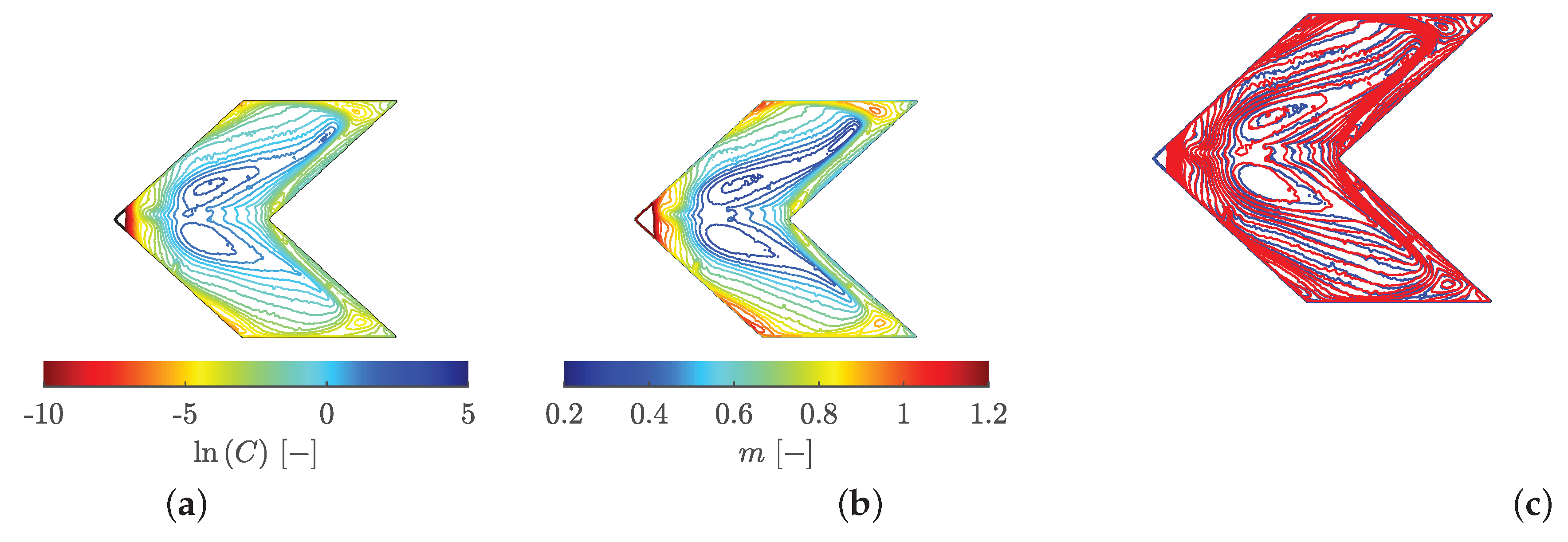
. Conversely, C shows an opposite trend, what is more clearly visible by the isoline representation of

ln (C)

and m in Figure 17a and b.

If the isolines of both distributions,

ln (C)

in red and m in blue, are superimposed (Figure 17c), the corresponding structure of both distributions is visible. The parallels to flow physics, as illustrated by oil visualization and the distribution m, were also noted by Terzis et al. [51] for a flow around obstacles or in multiple jet impingement situations [52].

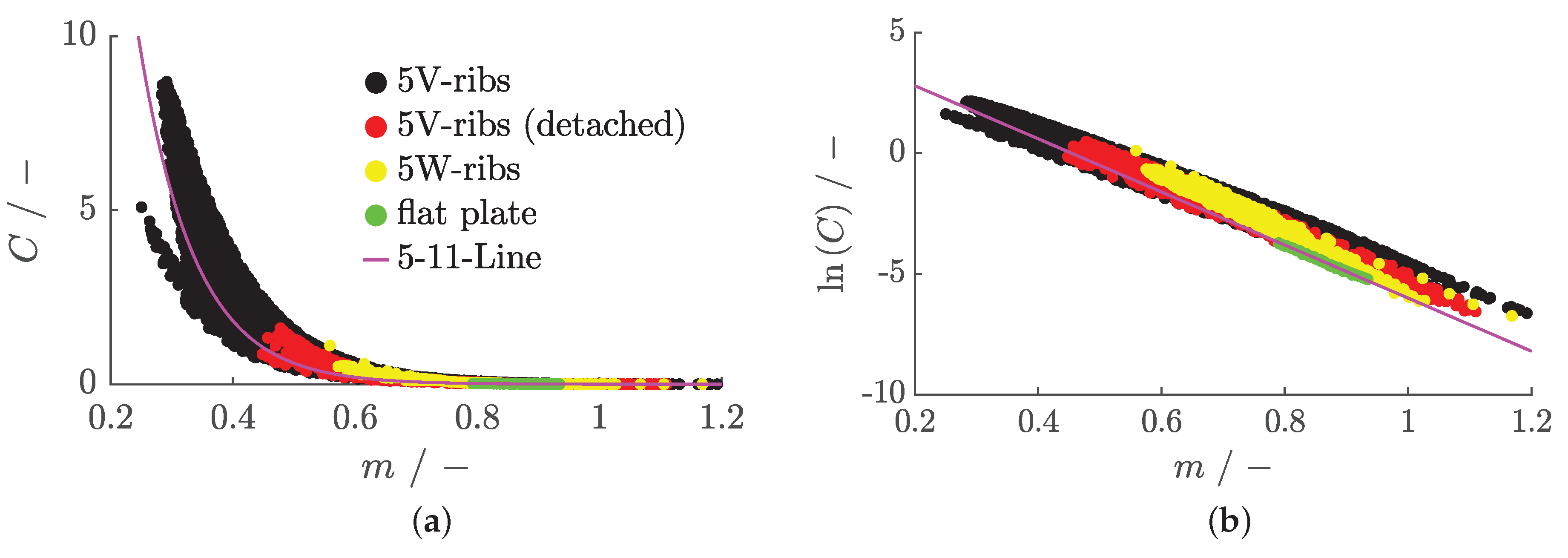
This complex flow situation significantly expands the C-m space, shown in Figure 18a. Here, the two-dimensional values from Figure 16 are presented with C over m and

β

as color information. Two branches are visible for

β < 1

and

β > 1

β

adjusts the dissipation component due to heat transfer or heat conduction but not the component due to kinematic heating. According to Rotta [53], the self-heating part cannot be guaranteed by

β

formulated in temperatures alone. For a comprehensive dissipation description, local velocities would also need to be included. However, since these velocities are indirectly present in the heat transfer data, their contribution might be hidden in C by the optimizer. Interestingly, the earlier found

A = 5

and

B = 11

from the data of the flat plate, are a good fit to the data of the ribbed geometry, holding

β \approx 1

(cf. Figure 18a).

However, one can argue from Figure 18b that a negative slope

B = 10.5

or an offset

A = 4.5

would be an equivalently reasonable fit. To investigate this further, similar to the flat plate, Equation 15 should therefore be optimized according to the parameters A, B, m and

β

. The parameters of the optimization for the initial values

A = 5

B = 11

m = 0.8

and

β = 1

are shown in Figure 19 as well as C calculated back from Equation 10. Analogous to the flat plate case, m and

β

remain unchanged optimizing Equation 9 or 15. The optimizer can “play” with the two new parameters A and B in such a way that the final result is the same C as with a direct optimization of C, m and

β

. The parameters A and B from the optimization with Equations 29, 28 and 32 result in f,

κ

and

ln ({Re}_{τ})

distributions, which are shown in Figure 20. All three distributions vary locally due to the dependence of A and B on the flow conditions and the pressure gradient. Because

ln (C)

is split into A and B using Equation 10, different combinations of A and B with the same m can result in the same C.

To analyze the dependency on initial values, different initial value combinations between

A = 4.5 . . 5.5

and

B = 10.5 . . 11.5

were chosen. The results are shown in Figure 21.

First of all, it is noticeable that the back-calculated C-distribution (a) and that for the parameter m (b) obtained directly from the optimization are independent of the initial value combination. Next, the physical quantities derived from A and B are investigated. In Figure 21c,

ln ({Re}_{τ})

is plotted against

ln (Re)

. The distribution varies depending on the initial value. The parameter range for

ln (Re)

increases with a larger initial value B. In contrast, the value of A determines the level of

{Re}_{τ}

and the range of

Re

, as curves with the same initial value A merge. Hereby, the initial value of parameter B exerts minimal influence on

ln ({Re}_{τ})

. Notably, when the friction factors from Equation 20 are normalized to the case with initial values

A = 5

and

B = 11

in Figure 21d, all f-values for

m = 1

coincide. For these, it is possible to combine all experimental Reynolds numbers from the different boundary condition courses to a unique solution, since for

m = 1

in Equation 34,

f / 2 = C

is independent of the Reynolds number. In consequence,

ln (C) = - 6 = A - B

must apply for

m = 1

. Since different Reynolds numbers occur in the different tests, there is no unique solution for

m \neq 1

and the optimizer searches for the nearest minimum depending on the initial values. However, for those m values, significant variations in f can be observed, with differences exceeding

50 %

for smaller m values.

Another approach to determine A and B without the dependency on initial values is shown in Figure 22a. For this, the more reliable parameters C and m from optimization of Equation 9 are used. In the A-B diagram, B is varied as a running variable and A is calculated for each B and each C-m-combination according to Equation 10. Different lines result for different evaluation points (see Figure 19). To determine A and B, the point on the straight line with the smallest distance from a target point is sought7 using the values of the flat plate (

A = 5

B = 11

), where Reynolds or Colburn analogy should hold. The advantage of the graphical solution is that there is a unique solution for A and B. To evaluate the different initial value combinations, the parameters from the optimization are compared with a correlation of Nagib and Chauhan8 [35], who investigated the dependence of

κ

and A with various pressure gradients. As can be seen in Figure 22b, the graphical solution lies best on the correlation of Nagib and Chauhan. The data from the optimization with the initial values

A = 5

and

B = 11

also lie mostly on the correlation curve and are the best approximation of the cases investigated. The other two data sets, which also fulfill the formal condition

A - B = - 6

for

m = 1

A = 4.5

B = 10.5

and

A = 5.5

B = 11.5

, deviate significantly more from the correlation curve.

An interpretation for the parameter m might be given following White and Christoph [54]. They investigated the influence of pressure gradient, heat transfer and compressibility for turbulent boundary layers on inner variables only, neglecting the “wake” flow effects. If all three vanish the logarithmic law, Equation 21, holds. Heating or favorable pressure gradients usually tend to depress the velocity profile, whereas cooling or adverse pressure gradients tend to raise the profile above the log law. The different effects can also compensate for each other, resulting in the log law again.

Figure 23 illustrates our interpretation of m, which occur locally depending on the flow situation and pressure gradient condition. For a flow without a pressure gradient, the velocity profile follows the log law, resulting in

m = 1

. For flows with a favorable pressure gradient, the profile flattens out; for flows with an adverse pressure gradient, it detaches, resulting in

m < 1

for favorable pressure gradients and

m > 1

for adverse pressure gradients.

Finally, to determine a more reliable friction factor f for a complex flow, the data from the C, m,

β

optimization are used in the following, because of their independence of initial values. As the data of parameter C might still be influenced of dissipation effects and in order to account for deviations from an analogy situation, the optimized C values are normalized to the 5-11 line. This results in

C_{n o r m}

C_{n o r m} = \frac{C}{exp (5 - 11 m)}

(42)

as a Reynolds analogy factor. Hence,

f_{n o r m}

is given by

f_{n o r m} = \frac{2 Nu}{Re \Pr^{1 / 3}} C_{n o r m} .

(43)

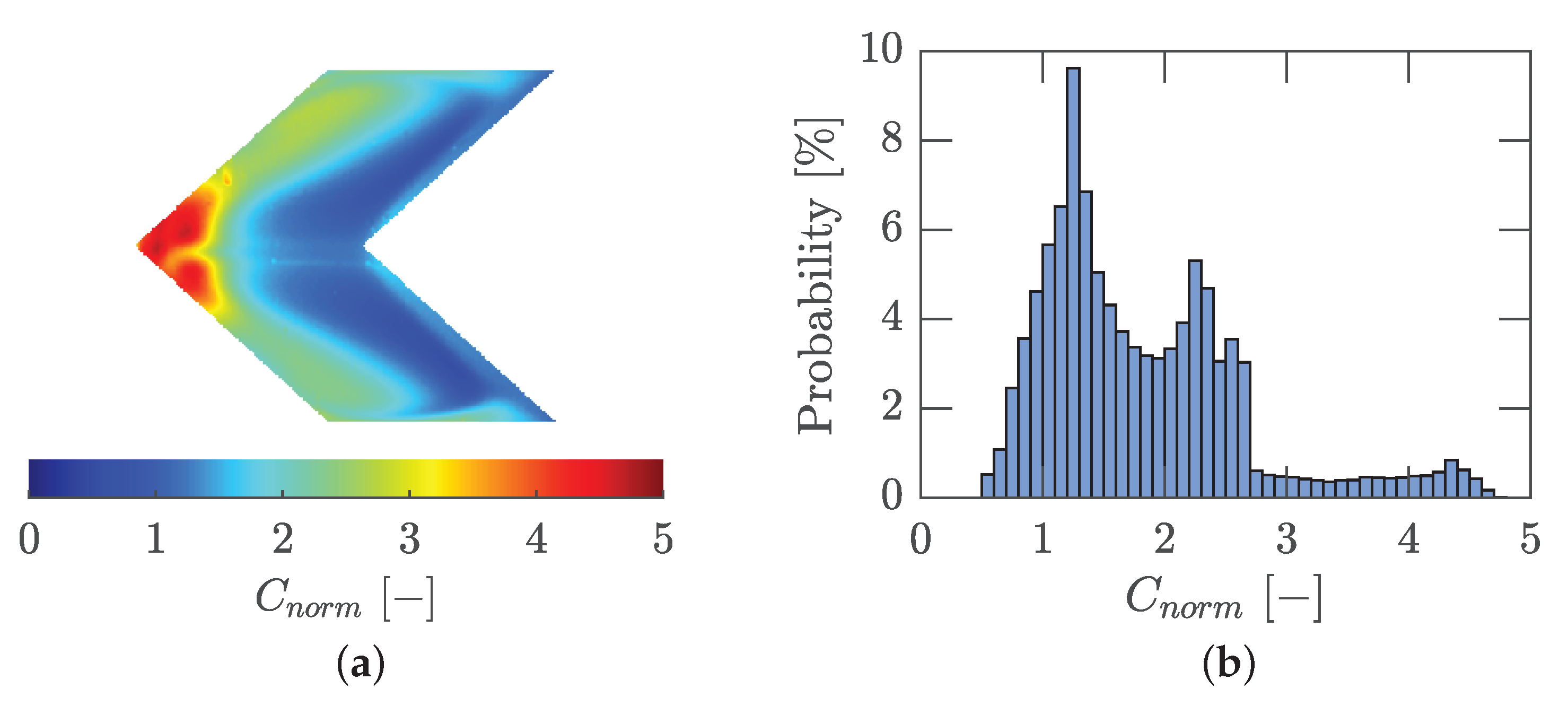
Figure 24a illustrates the surface distribution of

C_{n o r m}

, while Figure 24b presents a histogram of

C_{n o r m}

. In regions where

C_{n o r m} = 1

, the Reynolds or Colburn analogy

C = f / 2

formally holds. The range of

C_{n o r m}

extends to values around 5 in the area directly behind the ribs, aligning with the range reported by So [55] in his study on the effects of pressure gradients on the Reynolds analogy in equilibrium boundary layers. The minimum value of

C_{n o r m} \approx 0.5

would correspond to the lower boundary for Reynolds analogy factors found by So [55], which equates to a Clauser pressure parameter of approximately

- 0.5

. According to Mellor and Gibson [56], this is the smallest value at which equilibrium accelerated boundary layers still exist. In accelerated turbulent boundary layers,

C_{n o r m}

decreases, whereas it increases in regions with adverse pressure gradients.

By normalizing to the 5–11 line, a friction factor distribution can now be determined, what is shown in Figure 25a. Compared to the distribution calculated from Equation 20 with A and B in Figure 19, the range of values has been increased and the local flow effects taken into account. Furthermore, time-dependent distributions of wall shear stresses under various flow conditions can be calculated. Figure 25b presents this distribution for the Ramp B case (cf. Figure 3c) at

t = 150 s

. Additionally, Figure 25c depicts the temporal evolution of wall shear stress for four specific pixels, whose positions are indicated in Figure 25b.

To evaluate the quality of the wall shear stresses, the methodology presented was also applied to numerical conjugate heat transfer scenarios. Detailed information on the numerical model employed can be found in Hartmann et al. [2]. Figure 26a illustrates the wall shear stress calculated directly from the simulation, while Figure 26b shows

C_{n o r m}

obtained from the presented method using the numerically calculated heat transfer data. The resulting wall shear stress for the test case Ramp B after

t = 150 s

is depicted in Figure 26c.

The agreement between the wall shear stress obtained directly from the numerical simulation (Figure 26a) and that calculated from the simulations using the presented method (Figure 26c) is good. The largest deviations occur in the area immediately behind the rib, within the reattachment zone, and around the largest vortices. Similar deviations are observed in the distribution of wall temperatures, as reported by Hartmann et al. [2]. These discrepancies might be attributed to the isotropic model within the underlying SST turbulence model.

To investigate a more general validity of the method, two additional geometries were examined experimentally and the data processed the same way. First, the third V-rib on the plate, specifically the front rib in the field of view, was detached by

o = 5

mm. This adjustment aimed to weaken the recirculation areas due to the additional near-wall flow. Additionally, a case with five W-ribs instead of V-ribs was investigated. Both additional geometries were also measured experimentally under the presented boundary conditions (Figure 3a-h), and C, m and

β

were determined using Equation 9. The resulting distributions are shown in Figure 27.

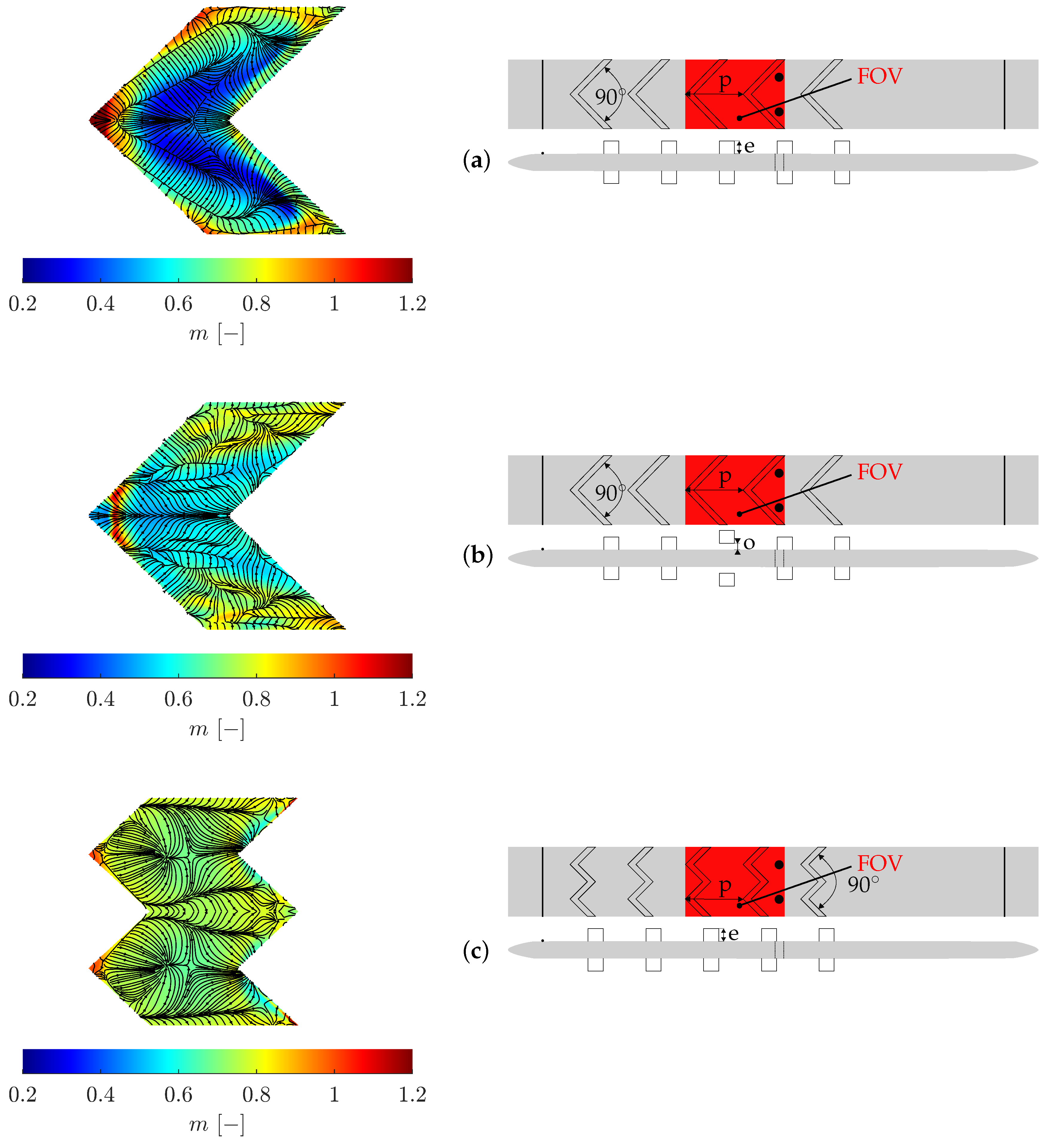
It is visible that the analyzed geometry with five periodically arranged V-ribs represents a somewhat extreme case that encompasses the value range of all other geometries. Detaching a rib doubles the smallest m and homogenizes the overall flow situation. While the geometry with five V-ribs clearly shows the formation of two branches, this is only slightly recognizable in the geometry with one detached rib. For the case with five W-ribs, larger detachment areas and reattachment zones are less recognizable, and the m range shifts toward the known coefficients for turbulent plate flow. The previously discussed 5-11 line fits all geometries well for

β \approx 1

To visualize the relationship between pressure gradient and m, pressure gradient streamlines from a numerical simulation are plotted over the m distribution of the experiment in Figure 28 for the attached (a) and detached (b) V-rib configurations as well as for the W-ribs (c). For the attached ribs, a deep valley with small m-values might be observed in the center of the field of view, with m values increasing towards the edges (see Figure 16b). The streamlines follow this trend, converging at the center point of lowest m. This close connection is even more evident with one detached rib. The additional flow below the front, detached rib creates a modified flow situation with several intermediate maxima at a more uniform m level overall. For constant m values in the center of the field of view, the streamlines converge. This phenomenon is also clearly observed in the W-ribs configuration, where the m distribution exhibits only slight variations across the entire field of view. In the regions behind the two imaginary V-ribs forming the W-rib, there is a small valley with lower m values compared to the rest of the field of view, where the pressure gradient streamlines converge. In the central area behind the W-rib, the streamlines run relatively undisturbed to the next rib at a constant

m \approx 0.8

, similar to the behavior observed in flat plate flow.

Previous analyses considered each pixel for the parameter optimization in isolation, without accounting for neighboring pixels. For an alternative method to describe the relationship between A and B, the information of the surrounding four pixels and therewith the spatial distribution is also be included. Therefore, the Equation 10 is differentiated with respect to m, resulting in

\frac{d C}{d m} = - B exp (A) exp (- m B) = - B C .

(44)

This approach allows for the direct calculation of B from C and its differential with respect to m. The gradients of both parameters C and m are computed via a central difference scheme.

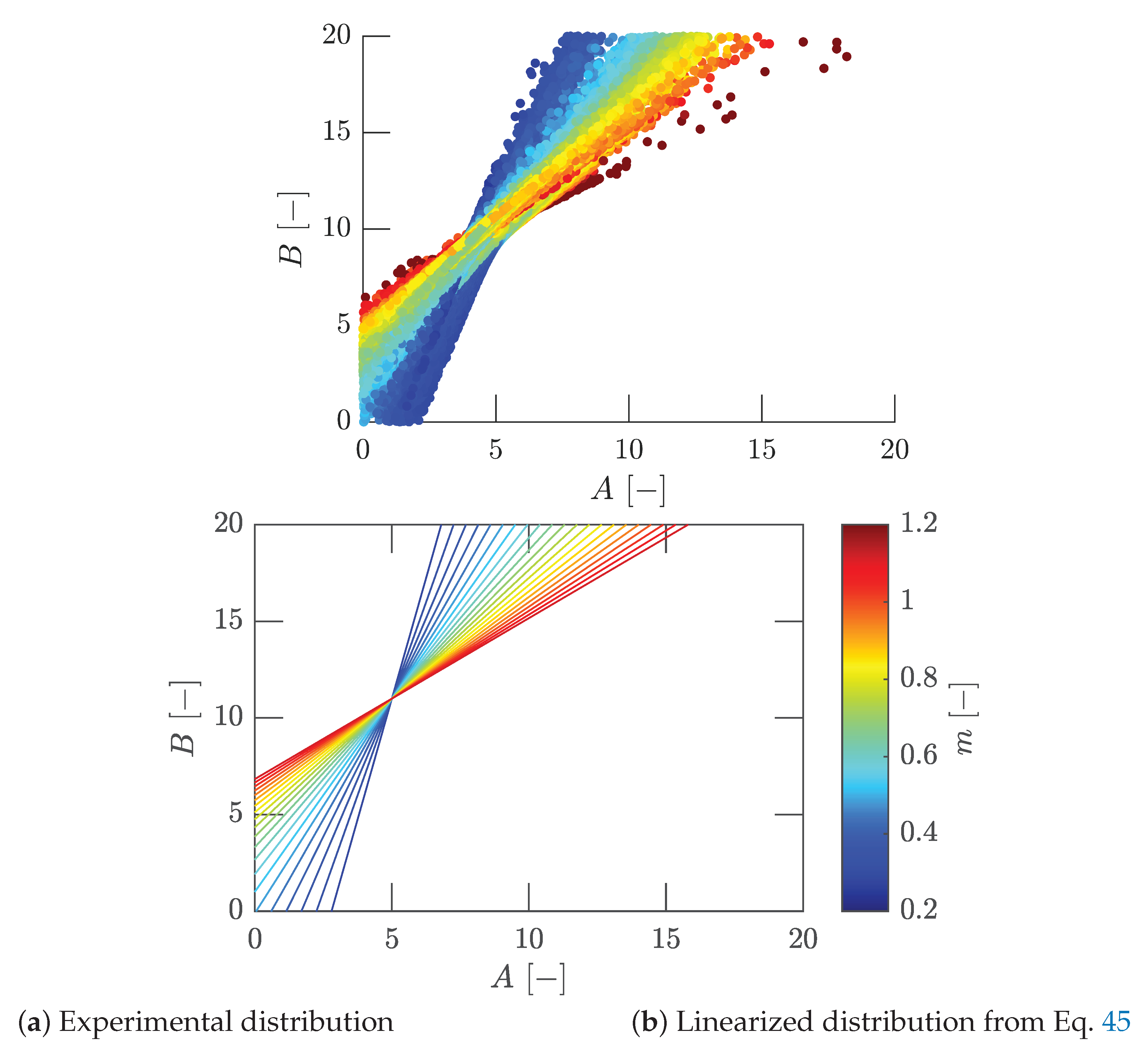
Figure 29 shows the resulting values of B over A and their histograms for the three geometries investigated. Here, A is calculated from C, m and B using Equation 10. The experimental values form a set of curves consisting of nearly straight lines as a function of m. These all intersect approximately around the common point

A \approx 5

and

B \approx 11

. The slight scattering around this point is presumably due to parameter C, which is still somewhat subject to dissipation. However, it is remarkable that all three distributions show a similar behavior independently of each other and that the majority of the points are grouped around

A \approx 5

and

B \approx 11

without any specifications regarding initial values.

This can also be seen in Figure 30a, where the experimental values of the geometries were plotted together with their respective m values. It results in a clear staggering of straight lines as a function of m, which can be described via

B = \frac{A - 5}{m} + 11,

(45)

where A is used as a running variable. Figure 30b shows Equation 45 as a set of ideal curves for different m. By definition, these intersect

A = 5

and

B = 11

, which in comparison with the results in Figure 30a directly from the differentiated experimental data, is again a very good approximation and unifies the observations of all investigated geometries. Hence, this is a further indicator for the choice of this characteristic point as a normalization condition.

4. Conclusions

An experimental test rig for transient conjugate heat transfer measurements was presented to investigated different time-varying temperature and velocity inlet boundary conditions using IRT. Spatially and temporally resolved heat fluxes were calculated using a semi-analytical approach for 3D heat conduction for a semi-infinite body by Estorf [7]. A method for determining adiabatic wall temperatures for constant inlet temperatures and inlet velocities was first extended for time-dependent temperature conditions using a regression plane and introducing a dissipation coefficient

β

. Subsequently, a quasi-steady model based on a typical heat transfer correlation was used assuming Reynolds similarity in the considered flow range. Solving the overdetermined system of equations at each pixel, result in a set of parameters C, m and

β

, whereas the first to mentioned strongly interact with each other. It was shown, that the model could reproduce the heat flux fairly.

The data set of perspex and quartz for a flat plate could described by the linear approximation

ln (C) = A - m B

, introducing the two new parameters A and B, representing the dimensionless gradient at the wall or an equivalent Reynolds number, respectively. With the definitions of the boundary layer variables, the parameters A and B were related to the log law variables as edge of the sublayer and matchpoint between inner law in the viscous sublayer and law of the wall, respectively. Subsequently, explicit relationships for Nusselt number and friction factor could be specified from A, B and the resulting von Kármán constant

κ

. A comparison with correlations in literature shows good agreement.

Next, a more complex flow of a V-rib geometry was investigated. Thus, C and m varied larger compared to the flat plate case, but show parallels to flow physics. m was linked to outer pressure gradient effects. For a flow without pressure gradients, this results in

m = 1

, for favorable pressure gradients in

m < 1

and for adverse pressure gradients in

m > 1

A sensitivity analysis for the optimization of A, B, m and

β

showed the strong dependence on the initial values of the optimization. To calculate the friction factor for complex flows, C, m and

β

were therefore used again and normalized to the case without pressure gradients. The line with

A = 5

and

B = 11

, i.e.

κ \approx 0.4

, was chosen as normalization. This line corresponds to

β \approx 1

. In addition, the line must pass through

A - B = - 6

for

m = 1

. The resulting

C_{n o r m}

is interpreted as a Reynolds analogy factor. Therefore local shear stress distributions could be evaluated. This was confirmed by the investigation of two other geometries introducing different pressure gradients. m is an indicator of the pressure gradients, which was shown by superimposing the streamlines of the pressure gradient from numerical simulations with the experimentally determined m distribution. Finally, for all cases using the spatial distributions of parameters C and m were analyzed with a numerical discretization scheme according to the model equation

ln (C) = A - m B

, which allowed to unify the observations for all geometries.

Author Contributions

Conceptualization, C.H. and J.v.W.; methodology, C.H., J.v.W.; software, C.H. and J.v.W.; validation, C.H. and J.v.W.; formal analysis, C.H. and J.v.W.; investigation, C.H.; resources, J.v.W.; data curation, C.H. and J.v.W.; writing—original draft preparation, C.H.; writing—review and editing, J.v.W.; visualization, C.H.; supervision, J.v.W.; project administration, J.v.W.; funding acquisition, J.v.W.. All authors have read and agreed to the published version of the manuscript.

Funding

The investigations were conducted as part of the joint research program KuepLe and DigiTecT in the frame of AG Turbo. The work was supported by the Federal Ministry for Economic Affairs and Climate Action (BMWK) as per resolution of the German Federal Parliament under grant numbers 0324358I and 03EE5117G.

Institutional Review Board Statement

Not applicable.

Informed Consent Statement

Not applicable.

Data Availability Statement

Not applicable.

Acknowledgments

Not applicable.

Conflicts of Interest

Not applicable.

Nomenclature and Abbreviations

The following nomenclature is used in this manuscript.

Roman characters

A	Parameter in −
B	Parameter in −
C	Pre-factor in Nusselt correlation in −
$c_{p}$	Specific heat capacity in $J k g^{- 1} K^{- 1}$
D	Pre-factor in power law in −
e	Characteristic rib height in $m$
f	Friction factor in −
h	Heat transfer coefficient in $W m^{- 2} K^{- 1}$
k	Thermal conductivity in $W m^{- 1} K^{- 1}$
L	Length in $m$
m	Exponent in Nusselt correlation in −
$Nu$	Nusselt number in −
o	Rib detachment in $m$
p	Pitch of ribs in $m$
$\Pr$	Prandtl number in −
$\dot{q}$	Heat flux in $W m^{- 2}$
$Re$	Reynolds number in −
$St$	Stanton number in −
t	Time in $s$
T	Temperature in $K$
u	Velocity in $m s^{- 1}$
$x, y, z$	Coordinates in $m$

Greek characters

$α$	Exponent in power law in −
$β$	Parameter for dissipation effects in −
$η$	Dynamic viscosity in $k g m^{- 1} s^{- 1}$
$κ$	von Kármán constant in −
$ν$	Kinematic viscosity in $m^{2} s^{- 1}$
$ρ$	Density in $k g m^{- 3}$
$τ$	Shear Stress in $k g m^{- 1} s^{- 2}$

Subscripts

+	Dimensionless
-	Effective
0	Initial
aw	Adiabatic wall
f	Fluid
norm	Normalization
ref	Reference
$τ$	Shear Stress
w	Wall

The following abbreviations are used in this manuscript:

CCT	Constant current thermometry
CTA	Constant temperature anemometry
Exp	Experiment
FOV	Field of view
IRT	Infrared thermography
Mod	Model
Num	Numeric

Notes

1	$f_{Blasius} = 0.0791 {Re}^{- 0.25}, Re < 10^{5}$
2	$f_{Nikuradse} = 0.046 {Re}^{- 0.2}, 3 \cdot 10^{4} < Re < 10^{6}$
3	$\frac{1}{\sqrt{4 f_{Prandtl}}} = 2 log (Re \sqrt{4 f_{Prandtl}}) - 0, 8$
4	$f_{Petukhov} = 2 {(2.236 ln (Re) - 4.639)}^{- 2}, 10^{4} < Re < 5 \cdot 10^{6}$
5	${Nu}_{Dittus - Boelter} = 0.023 {Re}^{0.8} \Pr^{0.3}, 0.6 < \Pr < 160, 10^{5} < Re$
6	${Nu}_{Kays et al .} = 0.022 {Re}^{0.8} \Pr^{M M 1 / 2}, 0.6 < \Pr < 6, 10^{4} < Re$
7	$\sqrt{{(A - 5)}^{2} + {(B - 11)}^{2}} = min$
8	$κ A = 1.6 (exp (0.1663 A) - 1)$

References

Perelman, T.L. On conjugated problems of heat transfer. International Journal of Heat and Mass Transfer 1961.
Hartmann, C.; Schweikert, J.; Cottier, F.; Israel, U.; Gier, J.; von Wolfersdorf, J. Experimental Validation of a Numerical Coupling Environment Applying FEM and CFD. International Journal of Turbomachinery, Propulsion and Power 2023.
Liu, C.; Gao, C.; von Wolfersdorf, J.; Zhai, Y. Numerical study on the temporal variations and physics of heat transfer coefficient on a flat plate with unsteady thermal boundary conditions. International Journal of Thermal Sciences 2017.
Esfahani, J.A.; Jafarian, M.M. Entropy Generation Analysis of a Flat Plate Boundary Layer with Various Solution Methods. Scientia Iranica 2005.
Moffat, R.J. What’s new in convective heat transfer? International Journal of Heat and Fluid Flow 1998.
Schlichting, H.; Gersten, K. Grenzschicht-Theorie. Springer-Verlag 2006.
Estorf, M. Image based heating rate calculation from thermographic data considering lateral heat conduction. International Journal of Heat and Mass Transfer 2006.
Liu, C.; von Wolfersdorf, J.; Zhai, Y. Time-resolved heat transfer characteristics for steady turbulent flow with step changing and periodically pulsating flow temperatures. International Journal of Heat and Mass Transfer 2014.
Brack, S.; Poser, R.; von Wolfersdorf, J. Experimental investigation of unsteady convective heat transfer under airflow velocity and temperature variations. Measurement Science and Technology 2021.
Moffat, R.J. Contributions to the Theory of Single-Sample Uncertainty Analysis. Journal of Fluids Engineering 1982.
Goldstein, R.J.; Eckert, E.R.G.; Ramsey, J.W. Film Cooling With Injection Through Holes: Adiabatic Wall Temperatures Downstream of a Circular Hole. Journal of Engineering for Power 1968.
Eckert, E.R.G. Cross transport of energy in fluid streams. Wärme- und Stoffübertragung 1987.
Bacci, T.; Picchi, A.; Facchini, B.; Cubeda, S. A New Experimental Approach for Heat Transfer Coefficient and Adiabatic Wall Temperature Measurements on a Nozzle Guide Vane With Inlet Temperature Distortions. Journal of Turbomachinery 2021.
Vinuesa, R.; Schlatter, P.; Nagib, H.M. Secondary flow in turbulent ducts with increasing aspect ratio. Physical Review Fluids 2018.
Kays, W.; Crawford, M.; Weigand, B. Convective Heat and Mass Transfer. McGraw-Hill Series in Mechanical Engineering 2005.
Sutherland, W. LII. The viscosity of gases and molecular force. The London, Edinburgh, and Dublin Philosophical Magazine and Journal of Science 1893.
White, F. Viscous fluid flow. McGraw-Hill Higher Education 2006.
Hetsroni, G.; Tiselj, I.; Bergant, R.; Mosyak, A.; Pogrebnyak, E. Convection Velocity of Temperature Fluctuations in a Turbulent Flume. Journal of Heat Transfer 2004.
Coleman, T.F.; Li, Y. On the convergence of interior-reflective Newton methods for nonlinear minimization subject to bounds. Mathematical Programming 1994.
Coleman, T.F.; Li, Y. An Interior Trust Region Approach for Nonlinear Minimization Subject to Bounds. SIAM Journal on Optimization 1996.
J. E. Dennis, Jr.; Schnabel, R.B. Nonlinear Least Squares Data Fitting. Numerical Methods for Unconstrained Optimization and Nonlinear Equations 1996.
Afzal, N. Scaling of Power Law Velocity Profile in Wall-bounded Turbulent Shear Flows. American Institute of Aeronautics and Astronautics 2005.
Dittus, F.W.; Boelter, L.M.K. Heat transfer in automobile radiators of the tubular type. International Communications in Heat and Mass Transfer 1985.
McAdams, W.H. Heat transmission. McGraw-Hill 1954.
Colburn, A.P. A method of correlating forced convection heat-transfer data and a comparison with fluid friction. International Journal of Heat and Mass Transfer 1964.
Blasius, H. Das Ähnlichkeitsgesetz bei Reibungsvorgängen in Flüssigkeiten. Mitteilungen über Forschungsarbeiten auf dem Gebiete des Ingenieurwesens 1913.
Nikuradse, J. Gesetzmäßigkeiten der turbulenten Strömung in glatten Rohren (Nachtrag). Forschung auf dem Gebiete des Ingenieurwesens 1933.
Prandtl, L. Zur turbulenten Strömung in Rohren und längs Platten. Ergebnisse der Aerodynamischen Versuchsanstalt zu Göttingen - IV. Lieferung 1932.
von Kármán, T. Mechanische Ähnlichkeit und Turbulenz. Nachrichten von der Gesellschaft der Wissenschaften zu Göttingen, Mathematisch-Physikalische Klasse 1930.
Coles, D. The law of the wall in turbulent shear flow. 50 Jahre Grenzschichtforschung 1955.
Reichardt, H. Vollständige Darstellung der turbulenten Geschwindigkeitsverteilung in glatten Leitungen. ZAMM - Journal of Applied Mathematics and Mechanics/Zeitschrift für Angewandte Mathematik und Mechanik 1951.
Spalding, D.B. A Single Formula for the “Law of the Wall”. Journal of Applied Mechanics 1961.
Meneveau, C. A note on fitting a generalised Moody diagram for wall modelled large-eddy simulations. Journal of Turbulence 2020.
Nickels, T.B. Inner scaling for wall-bounded flows subject to large pressure gradients. Journal of Fluid Mechanics 2004.
Nagib, H.M.; Chauhan, K.A. Variations of von Kármán coefficient in canonical flows. Physics of Fluids 2008.
Dixit, S.A.; Ramesh, O.N. Pressure-gradient-dependent logarithmic laws in sink flow turbulent boundary layers. Journal of Fluid Mechanics 2008.
Baxerres, V.; Vinuesa, R.; Nagib, H. Evidence of quasiequilibrium in pressure-gradient turbulent boundary layers. Journal of Fluid Mechanics 2024.
Petukhov, B.S. Heat Transfer and Friction in Turbulent Pipe Flow with Variable Physical Properties. Advances in Heat Transfer 1970.
Hussain, A.K.M.F.; Reynolds, W.C. Measurements in Fully Developed Turbulent Channel Flow. Journal of Fluids Engineering 1975.
Clark, J.A. A Study of Incompressible Turbulent Boundary Layers in Channel Flow. Journal of Basic Engineering 1968.
Afzal, N.; Seena, A.; Bushra, A. Power Law Velocity Profile in Fully Developed Turbulent Pipe and Channel Flows. Journal of Hydraulic Engineering 2007.
Barenblatt, G.I. Scaling laws for fully developed turbulent shear flows. Part 1. Basic hypotheses and analysis. Journal of Fluid Mechanics 1993.
Barenblatt, G.I.; Chorin, A.J.; Hald, O.H.; Prostokishin, V.M. Structure of the zero-pressure-gradient turbulent boundary layer. Proceedings of the National Academy of Sciences 1997.
Afzal, N.; Seena, A.; Bushra, A. Friction factor power law with equivalent log law, of a turbulent fully developed flow, in a fully smooth pipe. Zeitschrift für angewandte Mathematik und Physik 2023.
Barenblatt, G.I.; Chorin, A.J.; Prostokishin, V.M. A model of a turbulent boundary layer with a nonzero pressure gradient. Proceedings of the National Academy of Sciences 2002.
Barenblatt, G.I.; Chorin, A.J.; Prostokishin, V.M. Characteristic length scale of the intermediate structure in zero-pressure-gradient boundary layer flow. Proceedings of the National Academy of Sciences 2000.
Wosnik, M.; Castillo, L.; George, W.K. A theory for turbulent pipe and channel flows. Journal of Fluid Mechanics 2000.
Szablewski, W. Inkompressible turbulente Temperaturgrenzschichten mit konstanter Wandtemperatur. International Journal of Heat and Mass Transfer 1972.
van Driest, E.R. On Turbulent Flow Near a Wall. Journal of the Aeronautical Sciences 1956.
Cebeci, T.; Bradshaw, P. Physical and Computational Aspects of Convective Heat Transfer. Springer New York 1988.
Terzis, A.; von Wolfersdorf, J.; Weigand, B.; Ott, P. A method to visualise near wall fluid flow patterns using locally resolved heat transfer experiments. Experimental Thermal and Fluid Science 2015.
Terzis, A. On the correspondence between flow structures and convective heat transfer augmentation for multiple jet impingement. Experiments in Fluids 2016.
Rotta, J.C. Temperaturverteilungen in der turbulenten Grenzschicht an der ebenen Platte. International Journal of Heat and Mass Transfer 1964.
White, F.M.; Christoph, G.H. A Simple Theory for the Two-Dimensional Compressible Turbulent Boundary Layer. Journal of Basic Engineering 1972.
So, R.M.C. Pressure gradient effects on Reynolds analogy for constant property equilibrium turbulent boundary layers. International Journal of Heat and Mass Transfer 1994.
Mellor, G.L.; Gibson, D.M. Equilibrium turbulent boundary layers. Journal of Fluid Mechanics 1966.

Figure 1. Experimental setup.

Figure 2. Test geometries: (a) Flat plate. (b) Plate with V-shaped ribs.

(a) (b)

Figure 3. Boundary conditions: (a) Jump, (b) Ramp A, (c) Ramp B, (d) Pulsation A, (e) Pulsation B, (f) Cycle A, (g) Cycle B, (h) Cycle C, (i) Cycle D.

Figure 4. Determination of the adiabatic wall temperature for a constant inlet temperature and velocity. (a) Transient course of

{\dot{q}}_{w}

vs.

T_{w}

for Jump test case with

T_{f} = 323.15 K

. (b) Linear regression for four selected pixels. (c) Adiabatic wall temperature distribution for Jump test case with selected evaluation points.

Figure 4. Determination of the adiabatic wall temperature for a constant inlet temperature and velocity. (a) Transient course of

{\dot{q}}_{w}

vs.

T_{w}

for Jump test case with

T_{f} = 323.15 K

. (b) Linear regression for four selected pixels. (c) Adiabatic wall temperature distribution for Jump test case with selected evaluation points.

Figure 5. Determination of the adiabatic wall temperature at variable inlet temperature and constant inlet velocity at point P1 for perspex: (a) Pulsation A, (b) Ramp A, (c) Jump.

Figure 6. Adiabatic heat transfer coefficient (top) and dissipation coefficient (bottom) from slope-intercept form of a plane model for cases with varying fluid temperature at

u_{f} \approx 20 m s^{- 1}

: (a) Pulsation A, (b) Ramp A, (c) Jump.

Figure 6. Adiabatic heat transfer coefficient (top) and dissipation coefficient (bottom) from slope-intercept form of a plane model for cases with varying fluid temperature at

u_{f} \approx 20 m s^{- 1}

: (a) Pulsation A, (b) Ramp A, (c) Jump.

Figure 7. Parameter C, m and

β

from optimization of Equation 9.

Figure 7. Parameter C, m and

β

from optimization of Equation 9.

Figure 8. Dependence of the parameters C, m and

β

for (a) perspex or (b) quartz, respectively as well as histograms and mean values for C and m.

Figure 8. Dependence of the parameters C, m and

β

for (a) perspex or (b) quartz, respectively as well as histograms and mean values for C and m.

Figure 9. Comparison of the experimentally determined heat flux

{\dot{q}}_{w}

and the heat flux determined from the model according to Equation 9 for P1 for perspex over time of cases: (a) Jump, (b) Pulsation A, (c) Cycle D.

Figure 9. Comparison of the experimentally determined heat flux

{\dot{q}}_{w}

and the heat flux determined from the model according to Equation 9 for P1 for perspex over time of cases: (a) Jump, (b) Pulsation A, (c) Cycle D.

Figure 10. Comparison of the experimentally determined heat flux

{\dot{q}}_{w}

and the heat flux determined from the model according to Equation 9 for all pixel and time points of cases: (a) Jump, (b) Pulsation A, (c) Cycle D.

Figure 10. Comparison of the experimentally determined heat flux

{\dot{q}}_{w}

and the heat flux determined from the model according to Equation 9 for all pixel and time points of cases: (a) Jump, (b) Pulsation A, (c) Cycle D.

Figure 11. Dependence of the parameters C, m for perspex or quartz, respectively (a) and with

β

as color information (b).

Figure 11. Dependence of the parameters C, m for perspex or quartz, respectively (a) and with

β

as color information (b).

Figure 12. Parameter A, B, m and

β

and Histogram for A and B from optimization of Equation 15.

Figure 12. Parameter A, B, m and

β

and Histogram for A and B from optimization of Equation 15.

Figure 13. Characteristic velocity profile in a turbulent boundary layer in wall coordinates.

Figure 14. Comparison of Equation 29 (a) or Equation 30 (b) with literature.

Figure 15. Friction Reynolds number as a function of Reynolds number using

κ = \frac{1}{2.86}

Figure 15. Friction Reynolds number as a function of Reynolds number using

κ = \frac{1}{2.86}

Figure 16. Parameter C, m and

β

from optimization for the ribbed geometry.

Figure 16. Parameter C, m and

β

from optimization for the ribbed geometry.

Figure 17. Isolines for parameter

ln (C)

and m with spacing of

0.5

0.05

respectively as well as an overlay of both distributions for the ribbed geometry.

Figure 17. Isolines for parameter

ln (C)

and m with spacing of

0.5

0.05

respectively as well as an overlay of both distributions for the ribbed geometry.

Figure 18. Parameter C over m with

β

as color information (a) or with C plotted logarithmic (b) from optimization for the ribbed geometry.

Figure 18. Parameter C over m with

β

as color information (a) or with C plotted logarithmic (b) from optimization for the ribbed geometry.

Figure 19. Parameter A, B, m and

β

of the optimization and C calculated back from Equation 10.

Figure 19. Parameter A, B, m and

β

of the optimization and C calculated back from Equation 10.

Figure 20. Resulting f,

κ

and

ln ({Re}_{τ})

distributions from parameters A and B in Figure 19.

Figure 20. Resulting f,

κ

and

ln ({Re}_{τ})

distributions from parameters A and B in Figure 19.

Figure 21. Initial value variation for parameter A and B: Back-calculated C (a) and directly obtained m distribution (b).

ln ({Re}_{τ})

over

ln (Re)

(c), f over m normalized to the case (

A = 5

B = 11

) (d).

Figure 21. Initial value variation for parameter A and B: Back-calculated C (a) and directly obtained m distribution (b).

ln ({Re}_{τ})

over

ln (Re)

(c), f over m normalized to the case (

A = 5

B = 11

) (d).

Figure 22. Graphical solution to obtain initial value insensitivity (a) and

κ A

over A (b) using the correlation from Nagib and Chauhan [35]:

κ A = 1.6 (exp (0.1663 A) - 1)

Figure 22. Graphical solution to obtain initial value insensitivity (a) and

κ A

over A (b) using the correlation from Nagib and Chauhan [35]:

κ A = 1.6 (exp (0.1663 A) - 1)

Figure 23. Illustration of the effect of pressure gradients on m based on White and Christoph [54].

Figure 24.

C_{n o r m}

distribution as surface plot (a) or as histogram (b) for the ribbed geometry.

Figure 24.

C_{n o r m}

distribution as surface plot (a) or as histogram (b) for the ribbed geometry.

Figure 25. Friction factor f (a) and wall shear stress

τ_{w}

(b) at

t = 150 s

as surface plot or over t for case Ramp B (cf. Figure 3c) at four different pixels (c) for the ribbed geometry.

Figure 25. Friction factor f (a) and wall shear stress

τ_{w}

(b) at

t = 150 s

as surface plot or over t for case Ramp B (cf. Figure 3c) at four different pixels (c) for the ribbed geometry.

Figure 26. Wall shear stress distribution from the simulation for case Ramp B (cf. Figure 3c) at

t = 150 s

(a),

C_{n o r m}

distribution from the derived method for the numerical simulations (b) and resulting wall shear stress for the test case Ramp B (cf. Figure 3c) at

t = 150 s

(c).

Figure 26. Wall shear stress distribution from the simulation for case Ramp B (cf. Figure 3c) at

t = 150 s

(a),

C_{n o r m}

distribution from the derived method for the numerical simulations (b) and resulting wall shear stress for the test case Ramp B (cf. Figure 3c) at

t = 150 s

(c).

Figure 27. C-m-distribution and 5-11 line for different geometries with C (a) or

ln (C)

(b).

Figure 27. C-m-distribution and 5-11 line for different geometries with C (a) or

ln (C)

(b).

Figure 28. m-distribution of the experiments with superimposed streamlines from numerical simulations for the attached (a) or detached V-ribs (b) and W-ribs (c).

Figure 29. Dependency between A and B from spatial distribution of parameters C and m for the attached (a) or detached V-ribs (b) and W-ribs (c), respectively as well as histograms for parameters A and B.

Figure 30. Dependency between A and B from spatial distribution of parameters C and m for the experimental data (a) and a linearized distribution according to Equation 45 (b).

Disclaimer/Publisher’s Note: The statements, opinions and data contained in all publications are solely those of the individual author(s) and contributor(s) and not of MDPI and/or the editor(s). MDPI and/or the editor(s) disclaim responsibility for any injury to people or property resulting from any ideas, methods, instructions or products referred to in the content.

© 2024 by the authors. Licensee MDPI, Basel, Switzerland. This article is an open access article distributed under the terms and conditions of the Creative Commons Attribution (CC BY) license (http://creativecommons.org/licenses/by/4.0/).

Copyright: This open access article is published under a Creative Commons CC BY 4.0 license, which permit the free download, distribution, and reuse, provided that the author and preprint are cited in any reuse.

MDPI Initiatives

Important Links

Choose an area of interest and we will send you notifications of new preprints at your preferred frequency.

Disclaimer

Determination of Local Heat Transfer Coefficients and Friction Factors at Variable Temperature and Velocity Boundary Conditions for Complex Flows

Abstract

1. Introduction

2. Experimental Setup

3. Results

Method for Determining Adiabatic Wall Temperatures

Flat Plate Flow

Complex Flow Situations

4. Conclusions

Author Contributions

Funding

Institutional Review Board Statement

Informed Consent Statement

Data Availability Statement

Acknowledgments

Conflicts of Interest

Nomenclature and Abbreviations

Notes

References

MDPI Initiatives

Important Links

Subscribe