Tightness of Harary Graphs

Preprint

Article

Tightness of Harary Graphs

This version is not peer-reviewed.

This version is not peer-reviewed.

Altmetrics

Downloads

Views

Comments

Submitted:

14 August 2024

Posted:

16 August 2024

You are already at the latest version

A peer-reviewed article of this preprint also exists.

Abstract

In the design of real-world networks, researchers evaluate various structural parameters to assess vulnerability, including connectivity, toughness, and tenacity. Recently, the tightness metric has emerged as a potentially superior vulnerability measure, although many related theorems remain unknown due to its novelty. Harary graphs, known for their maximum connectivity, are an important class of graph models for network design. Prior work has evaluated the vulnerability of three types of Harary graphs using different parameters, but the tightness metric has not been thoroughly explored. This article aims to calculate the tightness values for all three types of Harary graphs. First, it will attempt to calculate the lower bound for the value of the tightness parameter in Harary graphs using existing lemmas and theorems. Then, by presenting new lemmas and theorems, we will try to find the exact value or upper bound for this parameter in Harary graphs. For the first type of Harary graph, the tightness is precisely determined, while for the second and third types, upper bounds are provided due to structural complexity. The lemmas, theorems, and proof methods presented in this research may be used to calculate other graph and network parameters. However, the newness of the tightness parameter means that further research is needed to fully characterize its properties.

Keywords:

Subject:

Computer Science and Mathematics - Applied Mathematics

1. Introduction

The concept of networks is prevalent across many scientific fields, and analyzing network characteristics is crucial. Parameters such as minimum and maximum degree, diameter, connectivity, clustering coefficient, and vulnerability level are commonly used to analyze networks modeled as graphs. Among these parameters, graph vulnerability parameters are particularly important. Vulnerability parameters aim to mathematically evaluate a graph or network’s weakest points by optimizing an objective function. This allows researchers to identify potential points of failure or instability within a network model. The analysis of network vulnerability is essential for designing robust and resilient real-world systems, whether in fields like communications, transportation, power grids, or social networks.

Some widely studied vulnerability parameters include: Connectivity (

κ

) [13,18,21,22], Toughness (t) [1,5,8,12,20], Tenacity (T) [2,17,19], Integrity (I) [6,7,17], Binding number (b) [1,4,23], and Scattering number (s) [14,16,17]. These parameters examine vulnerability from different perspectives. For example, toughness considers the number of cutting vertices and resulting components, while tenacity also incorporates the size of the largest remaining component.

The mathematical formulations of these vulnerability parameters are typically presented in both vertex-based and edge-based forms, depending on whether vertex cuts or edge cuts are being evaluated. Equations (1) and (2) respectively show the relationships of toughness and tenacity parameters in vertex mode, where

ω (G - C)

is the number of components and

τ (G - C)

is the largest component in

(G - C)

. Understanding and quantifying the vulnerability of networks using these graph theoretic parameters is crucial for designing robust real-world networks across various domains. The diversity of vulnerability metrics highlights the complexity of assessing network resilience.

t (G) = min_{C \subseteq V (G)} \{\frac{∥ C ∥}{ω (G - C)}\}

(1)

T (G) = min_{C \subseteq V (G)} \{\frac{∥ C ∥ + τ (G - C)}{ω (G - C)}\}

(2)

Evaluating the effectiveness of graph and network vulnerability parameters is a critical step in understanding their practical usefulness. Javan et al. [10] outlined several desirable characteristics that an effective vulnerability metric should possess. Drawing on this framework, they introduced a novel parameter called "tightness" that aims to embody these ideal properties as closely as possible.

The mathematical formulations for tightness in both the vertex-based and edge-based contexts are provided in Equations (3) and (4), respectively. These expressions leverage the ratio of the cut set size (

∥ C ∥

) to the number of removed paths, quantified as the difference between the total number of graph paths

(\binom{ν}{2})

and the sum of the path counts within each disconnected component

\sum_{i} (\binom{s_{i}}{2})

. This ratio reflects the cost-to-benefit tradeoff, where the numerator represents the cost of the cut and the denominator encapsulates the benefit in terms of disrupted paths.

Additionally, the inclusion of the total number of graph edges (

ε

) enhances the distinguishability of the tightness metric. Moreover, the incorporation of normalization coefficients (2,

ν

ν - 1

, where

ν

is the graph order) ensures that the metric exhibits desirable properties such as normality, comparability, monotonicity, unambiguity, and high distinguishability for connected graphs [10].

J (G) = min_{C \subseteq V (G)} \{\frac{2 ε ∥ C ∥}{ν ((\binom{ν}{2}) - \sum_{i = 1}^{ω (G - C)} (\binom{s_{i}}{2}))}\}

(3)

J_{e} (G) = min_{C \subseteq E (G)} \{\frac{2 ε ∥ C ∥}{ν (ν - 1) ((\binom{ν}{2}) - \sum_{i = 1}^{ω (G - C)} (\binom{s_{i}}{2}))}\}

(4)

By considering the constant values of

ε = ∥ E (G) ∥

and

ν = ∥ V (G) ∥

, and the function

f (G, C)

as defined in relation (5), we can simplify the mathematical formulations. Specifically, relations (3) and (4) can be rewritten as the more concise expressions (6) and (7), respectively. With these streamlined representations, the objective becomes minimizing the function

f (G, C)

, which captures the ratio of the cut set size C to the number of disrupted paths in

(G - C)

. This optimization problem reflects the fundamental tradeoff between the cost of the cut and the benefit of the resulting connectivity disruption.

f (G, C) = \frac{∥ C ∥}{(\binom{ν}{2}) - \sum_{i = 1}^{ω (G - C)} (\binom{s_{i}}{2})}

(5)

J (G) = \frac{2 ε}{ν} \times min_{C \subseteq V (G)} \{f (G, C)\}

(6)

J_{e} (G) = \frac{2 ε}{ν (ν - 1)} \times min_{C \subseteq E (G)} \{f (G, C)\}

(7)

In the design of real-world networks, assessing the vulnerability of those networks is of paramount importance. As such, calculating and comparing vulnerability parameters is a fundamental requirement when working with network models and graph structures.

To this end, researchers have extensively analyzed the vulnerability metrics across a diverse range of named graphs, including Harary [3,9,15], Cayley [11], bipartite [5], barbell [22], fuzzy [21], Kneser [20], and even random graphs [8].

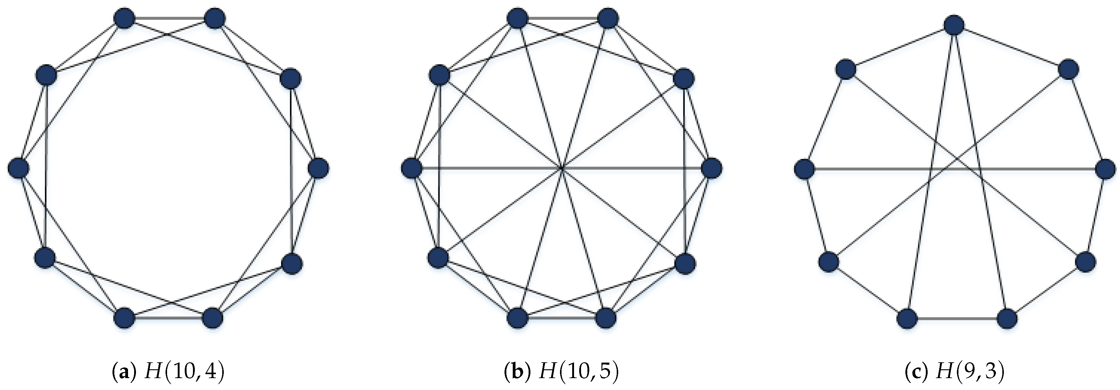
Notably, Harary graphs have emerged as a crucial tool for vulnerability analysis. These graphs, denoted as

H (n, m)

, represent a specific class of m-connected graphs with n vertices that possess the minimum possible number of edges [9]. This structural property makes Harary graphs an important model for studying vulnerability in real-world networks.These graphs are classified into three distinct types, depending on the number of vertices and the desired connectivity level (m). The edges in each Harary graph type is characterized by the following expressions, where the addition of indices is performed modulo n:

Type (a)m is even:

$E (H_{a} (n, m)) = ⋃_{i = 0}^{n - 1} \{⋃_{j = 1}^{m / 2} \{(v_{i}, v_{i + j})\}\}$

(8)
Type (b)m is odd and n is even:

$E (H_{b} (n, m)) = ⋃_{i = 0}^{n - 1} \{⋃_{j = 1}^{m / 2} \{(v_{i}, v_{i + j})\}\} \cup ⋃_{i = 0}^{(n - 2) / 2} \{(v_{i}, v_{i + n / 2})\}$

(9)
Type (c)m is odd and n is odd:

$E (H_{c} (n, m)) = ⋃_{i = 0}^{n - 1} \{⋃_{j = 1}^{m / 2} \{(v_{i}, v_{i + j})\}\} \cup ⋃_{i = 0}^{(n - 1) / 2} \{(v_{i}, v_{i + (n + 1) / 2})\}$

(10)

Figure 1 shows three example of these types of Harary graphs.

This study attempts to quantify the tightness parameter for three distinct classifications of Harary graphs. For this purpose, Section 2 uses relevant lemmas and results to derive upper bounds, lower bounds, and as accurate as possible values of this important parameter in three types of Harary graphs. Finally, the Conclusion section synthesizes the findings of this work and provides a comprehensive perspective on the significance and implications of our analysis. The obtained results may be used extensively in the design of real-world networks. Additionally, the methodologies presented could be valuable in proving related theorems in the field of graph theory.

2. Tightness of Harary Graphs

In this section, we will focus on different methods for evaluating the vulnerability of Harary graphs using the tightness parameter. Due to the varying structures of the three Harary graph types, distinct approaches will be required to calculate the tightness parameter values.

The lemmas, corollaries, and methodologies presented in this section may have broader applications beyond the specific context of Harary graphs. They could potentially be useful in solving other graph-theoretic problems and expanding the understanding of the tightness metric and its relationships with other graph parameters.

First, we will examine practical lemmas for finding the limits of tightness in Harary graphs. Lemma 1 shows the comparability property of the tightness parameter, as demonstrated in [10].

Lemma 1.

If G is a spanning subgraph of H, then

J (H) \geq J (G)

J_{e} (H) \geq J_{e} (G)

Theorem 1 also shows the value of tightness for cycle graphs [10].

Theorem 1.

C_{n}

is a cycle graph with n vertices (

n > 3

) then:

J (C_{n}) = \frac{4}{(\binom{n}{2}) - (\binom{⌊ \frac{n - 2}{2} ⌋}{2}) - (\binom{⌈ \frac{n - 2}{2} ⌉}{2})}

Based on Lemma 1 and Theorem 1 the Corollary 1 can be derived.

Corollary 1.

If G is Hamiltonian, then:

J (G) \geq \frac{4}{(\binom{n}{2}) - (\binom{⌊ \frac{n - 2}{2} ⌋}{2}) - (\binom{⌈ \frac{n - 2}{2} ⌉}{2})}

Harary graphs are Hamiltonian for

n > m \geq 2

. Therefore, Corollary 1 holds for Harary graphs and can be writen as Corollary 2.

Corollary 2.

H (m, n)

is a Harary graph with n vertices and connectivity m, then:

J (H (m, n)) \geq \frac{4}{(\binom{n}{2}) - (\binom{⌊ \frac{n - 2}{2} ⌋}{2}) - (\binom{⌈ \frac{n - 2}{2} ⌉}{2})}

The calculation of more accurate bounds can also be achieved by using the relationship between tightness and the rest of the graph parameters. For example, the connectivity of Harary graphs is equal to m. This problem shows that in order to divide the graph into two parts, we need to remove at least m vertices. Therefore, to find the upper limit, it is possible to establish a relationship between tightness and connectivity. Theorem 2 shows the relationship between tightness and connectivity.

Theorem 2.

H (m, n)

is a Harary graph with n vertices and connectivity m, then:

J (H (n, m)) \leq \frac{2 m^{2}}{2 n m - m^{2} + 2 n - 3 m - 2}

Proof.

The connectivity of Harary graphs is m. Therefore, by removing m vertices from these types of graphs, the graph can be divided into smaller components. Increasing the number of components causes the loss of more paths in the graph and reduces the objective function of the tightness parameter. Thus, to find an reliable upper bound, we consider the worst case of this division. Therefore, we consider that two components created by removing m vertices from the Harary graphs as

s_{i}

and

s_{j}

. With this method, the objective function can be expressed as Equation (11), where

∥ C ∥ = m

and

s_{i} + s_{j} = n - m

\begin{matrix} f (H (n, m), C) & = \frac{m}{(\binom{n}{2}) - ((\binom{s_{i}}{2}) + (\binom{s_{j}}{2}))} \\ = \frac{2 m}{n^{2} - n - s_{i}^{2} + s_{i} - s_{j}^{2} + s_{j}} \\ = \frac{2 m}{n^{2} - n - s_{i}^{2} + s_{i} - {(n - m - s_{i})}^{2} + (n - m - s_{i})} \\ = \frac{2 m}{2 n m - m^{2} - m + 2 s_{i} (n - m - s_{i})} \end{matrix}

(11)

Considering fixed values for n and m, the maximum value of the objective function in relation (11) occurs when the denominator of the fraction has its smallest value.

The minimum value of the denominator of the Equation (11) also occurs when

2 s_{i} (n - m - s_{i})

becomes minimum. The minimum value for

2 s_{i} (n - m - s_{i})

also occurs when

s_{i} = 1

s_{i} = n - m - 1

. As shown below, the value of the objective function will be the same for any initialization of

s_{i}

\begin{matrix} s_{i} = 1 \Rightarrow 2 s_{i} (n - m - s_{i}) = 2 (n - m - 1) \\ s_{i} = n - m - 1 \Rightarrow 2 s_{i} (n - m - s_{i}) = 2 (n - m - 1) \end{matrix}

Therefore, the upper bound for the objective function

f (H (n, m))

and

J (H (n, m))

can be expressed by Equations (12) and (13), respectively.

f (H (n, m), C) \leq \frac{2 m}{2 n m - m^{2} + 2 n - 3 m - 2}

(12)

J (H (n, m)) \leq \frac{2 m^{2}}{2 n m - m^{2} + 2 n - 3 m - 2}

(13)

□

In this section, the upper and lower bounds for tightness of Harary graphs were calculated approximately. In the following, we will take a closer look at tightness values for these types of graphs.

2.1. Tightness of Harary Graphs Type (a)

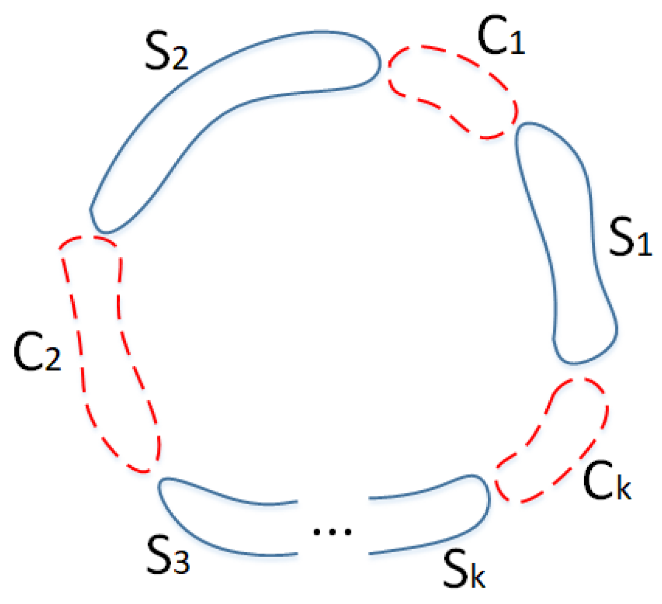
In our analysis of Harary graphs of type (a), we consider the scenario where certain sets of vertices, denoted as

C_{i}

, are removed in order to calculate the value of the tightness parameter

J (G)

. Correspondingly, other sets of vertices, denoted as

S_{j}

, remain in the graph as connected components. For the sake of simplicity, we assume that the indices of the vertices within each deleted set

C_{i}

and each remaining component

S_{j}

are consecutive. The validity of this approach will be established through a series of rigorous lemmas and corollaries presented in the subsequent sections. Consequently, we can define a set S comprising all the vertices belonging to the remaining components

S_{j}

, as well as a cut set C encompassing all the deleted vertex sets

C_{i}

. With this vertex cut in place, we can further partition the paths removed from the Harary graph of type (a) into three distinct categories:

P (C, C)

P (C, S)

, and

P (S, S)

. The value

P (C, C)

represents the deleted paths connecting vertices within the cut set C,

P (C, S)

denotes the deleted paths between vertices in the cut set C and the vertices in the remaining components S, and

P (S, S)

corresponds to the deleted paths between vertices within the components S.

Moreover, for the removal of a set of vertices in the Harary graphs of type (a) to successfully separate two components, the cardinality of each cut set

C_{i}

must be greater than or equal to

m / 2

, where m is the desired connectivity for Harary graph.

Equations (14) through (17) provide the mathematical formulations of these variables, where

c_{i} = ∥ C_{i} ∥

s_{i} = ∥ S_{i} ∥

c = ∥ C ∥

s = ∥ S ∥

, and k is the number of remaining components.

C = ⋃_{i = 1}^{k} C_{i}, S = ⋃_{i = 1}^{k} S_{i}

(14)

P (C, C) = (\binom{c}{2}) = \frac{c^{2} - c}{2}

(15)

P (C, S) = c s

(16)

P (S, S) = \sum_{i = 1}^{k - 1} \sum_{j = i + 1}^{k} s_{i} s_{j}

(17)

To determine the tightness of Harary graphs of type (a), we will seek to minimize the objective function denoted as

f (G, C)

. This objective function can be expressed in terms of the previously defined sets C and S, as shown in Equation (18).

\begin{matrix} f (H_{a} (n, m), C) & = \frac{∥ C ∥}{P (C, C) + P (C, S) + P (S, S)} \\ = \frac{c}{(c^{2} - c) / 2 + c s + \sum_{i = 1}^{k - 1} \sum_{j = i + 1}^{k} s_{i} s_{j}} \end{matrix}

(18)

To determine the minimum value of the function

f (G, C)

, we must first establish several foundational lemmas. Lemma 2 will demonstrate that the size of the components must be sufficiently small in order to minimize the values of

f (G, C)

. The proof of this key lemma will illuminate the underlying structure and properties of the function

f (G, C)

, providing crucial insights that will guide us towards the global minimum.

Lemma 2.

If, after identifying the vertex cut set C in Harary graphs of type (a), we obtain

f (G, C) = a / b

, then the value of

f (G, C)

is not at its minimum if the size of the largest component is greater than

b / a + 1

Proof.

Suppose that a vertex v is removed from a component

S_{i}

. The number of new deleted paths will be at least

s_{i} - 1

, where

s_{i} = ∥ S_{i} ∥

. If v is a cut vertex, then the number of new deleted paths will be greater than

s_{i} - 1

. Therefore, to maximize the number of deleted paths, it is optimal to select this vertex from the largest component. Consequently, the ratio of the number of deleted vertices to the number of deleted paths will be equal to

1 / (s_{m a x} - 1)

, where

S_{m a x}

is the largest component of

(G - C)

and

s_{m a x} = ∥ S_{m a x} ∥

Given that

s_{m a x} > b / a + 1

, and denoting

P = P (C, C) + P (C, S) + P (S, S)

and

c = ∥ C ∥

, using relations (19) ,we can conclude that the value of objective function

f (G, C)

is not at its minimum.

\begin{matrix} s_{m a x} > \frac{b}{a} + 1 \Rightarrow s_{m a x} - 1 > \frac{b}{a} = \frac{P}{c} \Rightarrow (s_{m a x} - 1) c > P \\ \Rightarrow (s_{m a x} - 1) c + P c > P + P c \Rightarrow c (P + s_{m a x} - 1) > P (c + 1) \\ \Rightarrow \frac{c}{P} > \frac{c + 1}{P + s_{m a x} - 1} \Rightarrow f (G, C) > f (G, C + v) \end{matrix}

(19)

□

Therefore, by repeatedly removing vertices from the largest component of Harary graphs type (a), when the size of the component exceeds the desired limit, we can reduce the value of the objective function.

This repetition may causes large components to be divided into smaller components. The vertices removed from this component, if they create a cut, in addition to the removed paths between C vertices, they also destroy the path between some

S_{m a x}

vertices. This will lead to a decrease in the value of

f (G, C)

. Although Lemma 2 does not give us a general view of the optimal tightness value, it can be used for a superficial examination of the results obtained from the calculations.

According to Lemma 2, after reducing the objective function

f (G, C)

, if there is a cut vertex within any component

S_{i}

, the cut vertex can be replaced with its right or left vertex and this can be done until the index of the cut vertices as well as the index of the components became consecutive. Thus, the following corollary can be derived:

Corollary 3.

In Harary graphs of type (a), the indices of the vertices of each component

S_{i}

and each cut set

C_{i}

can be considered consecutive to find the minimum value of

f (G, C)

Figure 2 shows a desirable partition for Harary graphs type (a) based on mentioned lemmas and corollaries.

Considering the fixed number of cutting vertices, to minimize the objective function

f (H_{a} (n, m), C)

P (S, S)

must be maximized. To maximize

P (S, S)

, the size difference of the generated components should be minimized. In other words, the size difference of all created components must be at most 1. This issue has been studied under Lemma 3.

Lemma 3.

With a constant number of cutting vertices in

H_{a} (n, m)

, the minimized value of

f (H_{a} (n, m), C)

occurs when

\forall 1 \leq i, j \leq k : ∥ s_{i} - s_{j} ∥ \leq 1

, where k is the number of remaining components after the cut, and

s_{i}

and

s_{j}

are the sizes of the i-th and j-th components, respectively.

Proof.

To minimize the objective function

f (H_{a} (n, m), C)

P (S, S)

must be maximized. Suppose there are two components

S_{p}

and

S_{q}

with sizes

s_{p}

and

s_{q}

, respectively, where

∥ s_{p} - s_{q} ∥ > 1

. Without loss of generality, suppose that

s_{p} > (s_{q} + 1)

(s_{p} - s_{q} - 1) > 0

By removing a vertex from the larger component and adding a vertex to the smaller component, we actually shift the vertices between them (cut sets and components) by one vertex towards the larger component. With this, the value of

P (S, S)

changes in the form of Equation (20), which indicates the increase of this value.

\begin{matrix} P_{n e w} (S, S) & = \sum_{i = 1}^{k - 1} \sum_{j = i + 1}^{k} s_{i} s_{j} \\ = (\sum_{\begin{matrix} i = 1 \\ i \neq p \\ i \neq q \end{matrix}}^{k - 1} \sum_{\begin{matrix} j = i + 1 \\ i \neq p \\ i \neq q \end{matrix}}^{k} s_{i} s_{j}) + ((s_{p} - 1) \sum_{\begin{matrix} i = 1 \\ i \neq p \\ i \neq q \end{matrix}}^{k} s_{i}) + ((s_{q} + 1) \sum_{\begin{matrix} j = 1 \\ j \neq p \\ j \neq q \end{matrix}}^{k} s_{j}) + (s_{p} - 1) (s_{q} + 1) \\ = (\sum_{\begin{matrix} i = 1 \\ i \neq p \\ i \neq q \end{matrix}}^{k - 1} \sum_{\begin{matrix} j = i + 1 \\ i \neq p \\ i \neq q \end{matrix}}^{k} s_{i} s_{j}) + (s_{p} \sum_{\begin{matrix} i = 1 \\ i \neq p \\ i \neq q \end{matrix}}^{k} s_{i}) + (s_{q} \sum_{\begin{matrix} j = 1 \\ j \neq p \\ j \neq q \end{matrix}}^{k} s_{j}) + s_{p} s_{q} + (s_{p} - s_{q} - 1) \\ = P (S, S) + (s_{p} - s_{q} - 1) > P (S, S) \end{matrix}

(20)

By repeating the operation of removing a vertex from the largest component and adding it to the smallest one, the upward trend of

P (S, S)

will continue. This operation can be done until the size of the components are almost balanced, or in other words,

\forall 1 \leq i, j \leq k : ∥ s_{i} - s_{j} ∥ \leq 1

. This ensures the minimization of the size difference between the components, which in turn maximizes

P (S, S)

and minimizes the objective function

f (H_{a} (n, m), C)

. □

Using Lemma 3, and assuming continuous values for c, s, and k, the Equation (18) can be written as Equation (21).

\begin{matrix} f_{C o n t i n u o u s} (H_{a} (n, m), C) & = \frac{c}{(c^{2} - c) / 2 + c s + \sum_{i = 1}^{k - 1} \sum_{j = i + 1}^{k} {(\frac{s}{k})}^{2}} \\ = \frac{c}{(c^{2} - c) / 2 + c s + ((k^{2} - k) / 2) {(\frac{s}{k})}^{2}} \\ = \frac{2 c}{c^{2} - c + 2 c s + (k^{2} - k) {(\frac{s}{k})}^{2}} \end{matrix}

(21)

Given the fact that

c + s = n

, the Equation (21) can be rewritten in terms of c as Equation (22).

\begin{matrix} f_{C o n t i n u o u s} (H_{a} (n, m), C) & = \frac{2 c}{c^{2} - c + 2 c (n - c) + (k - 1) (\frac{{(n - c)}^{2}}{k})} \\ = \frac{2 c}{2 n c - c^{2} - c + \frac{k - 1}{k} {(n - c)}^{2}} \end{matrix}

(22)

By differentiating the continuous function in Equation (22) with respect to the variable c (

d f_{c o n t i n u o u s} / d c = 0

), the extremum value is obtained as

c = \pm n \sqrt{1 - k}

. However, these obtained values are not acceptable while

k > 1

. Therefore, the continuous function in Equation (22) will be either ascending or descending.

Assigning 0 and n to the variable c, the obtained values are 0 and

2 / (n - 1)

, respectively. Thus, to minimize the value of the function in Equation (22), the value of c must be minimized. Additionally, the minimum value of c is achieved when the cut occurs, i.e.,

c = m

. Furthermore, the minimum value of

c = m

makes the value of k equal to 2. Therefore, the continuous function in Equation (22) can be written as Equation (23).

\begin{matrix} f_{C o n t i n u o u s} (H_{a} (n, m), C) & = \frac{2 m}{2 n m - m^{2} - m + \frac{1}{2} {(n - m)}^{2}} \end{matrix}

(23)

Although the calculations of the tightness value of Herary graphs type (a) have been done accurately and by mathematical relations, we can still use Lemma 2 to re-examine the results. The size of the largest component with this cut will be

s_{m a x} = ⌈ (n - m) / 2 ⌉

, and

⌈ (n - m) / 2 ⌉ \leq 1 / f_{Continuous} (H_{a} (n, m), C) + 1

. Therefore, based on Lemma 2, there is no need to add a new vertex to the cut set.

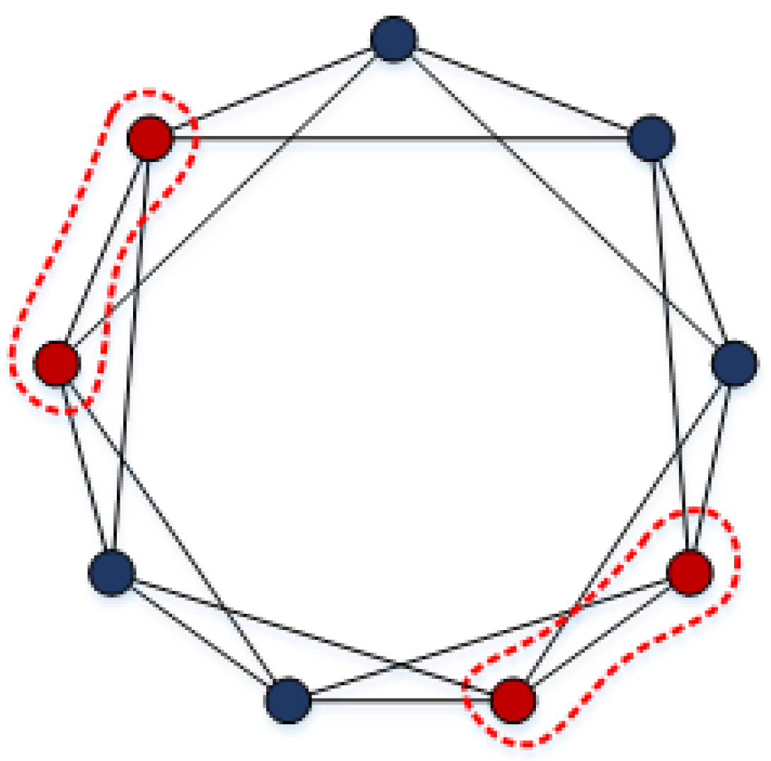
Accordingly, to calculate the tightness of Harary graphs type (a), two components, as large as possible, with minimum different sizes have to be created after cutting. Therefore, based on the previous lemmas and corollaries, having

ν = n

and

ε = n m / 2

f (H_{a} (n, m), C)

and

J (H_{a} (n, m))

can be written as Equations (24) and (25) in the discrete space, respectively. Figure 3 shows an optimal cut for calculating

J (H (9, 4))

\begin{matrix} min_{C \subseteq V (H_{a} (n, m))} {f (H_{a} (n, m), C)} & = \frac{2 m}{2 n m - m^{2} - m + 2 (⌊ \frac{n - m}{2} ⌋ \times ⌈ \frac{n - m}{2} ⌉))} \end{matrix}

(24)

\begin{matrix} J (H_{a} (n, m)) = \frac{n m}{n} & \times (\frac{2 m}{2 n m - m^{2} - m + 2 (⌊ \frac{n - m}{2} ⌋ \times ⌈ \frac{n - m}{2} ⌉)}) \\ = (\frac{2 m^{2}}{2 n m - m^{2} - m + 2 (⌊ \frac{n - m}{2} ⌋ \times ⌈ \frac{n - m}{2} ⌉)}) \end{matrix}

(25)

2.2. Tightness of Harary Graphs Types (b) and (c)

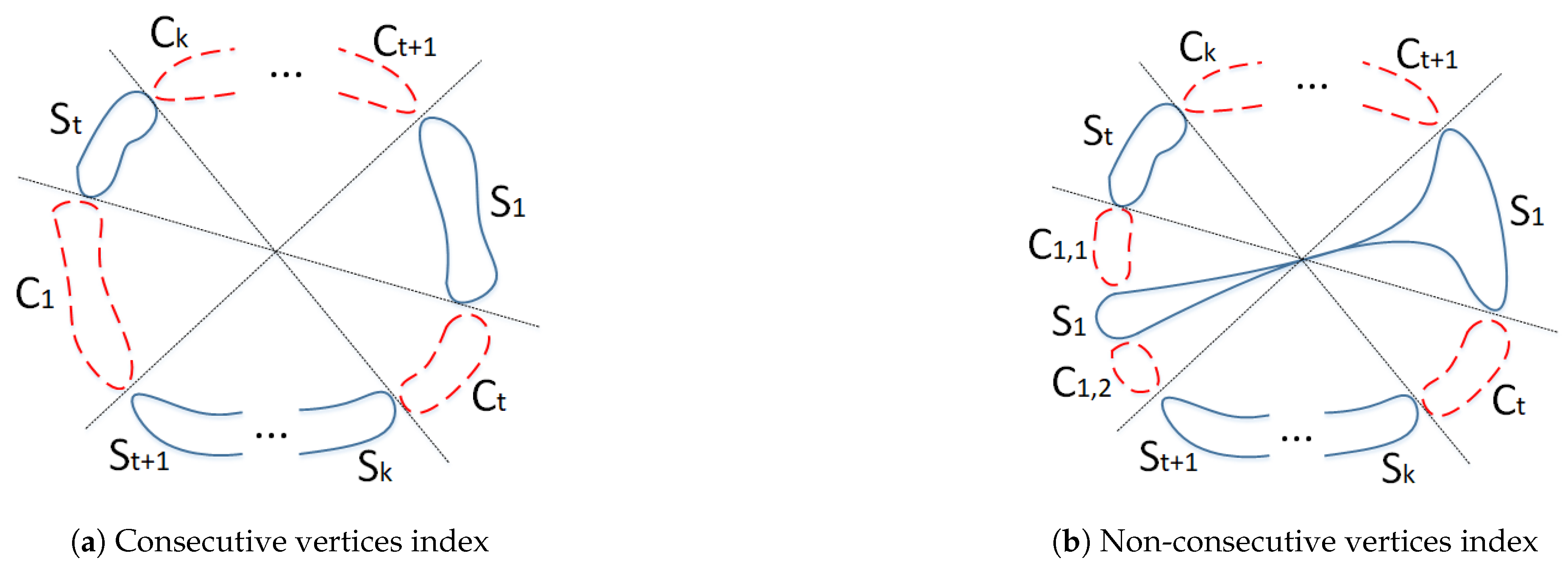
Calculating the tightness value of Harary graphs type (a) required intricate mathematical relationships and theorems. In contrast, Harary graphs types (b) and (c) possess more complex structures, suggesting that determining their tightness values would be far more arduous. As illustrated in Figure 4, obtaining an optimal vertex cut is exceptionally challenging for these two graph types, as each vertex is connected to its opposite counterpart. This cut can be executed in two ways: by either completely removing the opposite vertices, as shown in Figure 4a, resulting in a consecutiveness vertices index for the component, or by partially removing them, as depicted in Figure 4b, leading to a non-consecutiveness vertices index for the component. Both approaches increase the complexity of the problem significantly.

Therefore, in this section, we will endeavor to provide a suitable upper bound for the tightness value of Harary graphs types (b) and (c). Based on the calculated tightness for Harary graphs type (a), it can be concluded that this parameter does not increase the number of components in the graph.

Accordingly, to find a good upper bound for the tightness parameter in Harary graphs types (b) and (c), suppose we want to split the graph into two components. Therefore, separating one component from the graph makes the rest of the graph contain at least one other component. So, to calculate a good upper bound, we will focus on isolating a component from the graph.

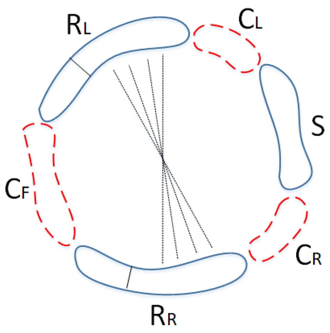
Figure 5 shows the general state of this separation, in which the set of vertices S represents the desired component, while the sets of vertices

C_{R}

C_{L}

, and

C_{F}

are the cut vertices on the right, left, and opposite sides of the desired component, respectively.

By removing the cut vertices

C_{R}

C_{L}

, and

C_{F}

, the removed paths are divided into three sections:

P (C, C)

P (C, S \cup R)

, and

P (S, R)

, where

C = C_{R} \cup C_{L} \cup C_{F}

, S is the component, and R is the remaining vertices after cutting, or

R = V (G) - C - S

. In the continuation of the process of finding the upper bound for the tightness of Harary graphs types (b) and (c), we will assume that R are connected, or in other words,

P (R, R) = 0

Suppose that

s = ∥ S ∥ \leq m

, then

C_{F} \geq s

, and to decrease the number of cut vertices (

∥ C ∥

) we can assume that

C_{F} = s

. Note that the value of

s > m

allows us to add a part of the cutting vertices of

C_{F}

to reduce the number of cutting vertices to the set of S. This state is shown in Figure 4.

In addition, to minimize the number of cutting vertices, the values of

C_{L}

and

C_{R}

must be equal to

(m - 1) / 2

. With these explanations, the values of

P (C, C)

P (C, R \cup S)

, and

P (S, R)

can be written as Equations (26), (27), and (28), respectively.

P (C, C) = (\binom{m - 1 + s}{2}) = \frac{(m + s - 1) (m + s - 2)}{2}

(26)

P (C, R \cup S) = (m + s - 1) (n - m + 1 - s)

(27)

P (S, R) = s (n - m - 2 s + 1)

(28)

Therefore, the objective function can be expressed as Equation (29).

\begin{matrix} f (H_{b} (n, m), C) = \frac{∥ C ∥}{P (C, C) + P (C, R \cup S) + P (S, R)} \\ = \frac{m + s - 1}{(m + s - 1) (m + s - 2) / 2 + (m + s - 1) (n - m + 1 - s) + s (n - m - 2 s + 1)} \\ = \frac{2}{(m + s - 2) + 2 (n - m + 1 - s) + 2 s (n - m - 2 s + 1) / (m + s - 1)} \\ = \frac{2}{2 n - 3 s - m + 2 s (n - s) / (m + s - 1)} \end{matrix}

(29)

The values of n and m in relation (29) are constant. Therefore, it is possible to find the extremum point by differentiating the objective function

f (G, C)

with respect to s, if it exists. By this method, the extremum point will be as Equation (30). Thus, an extremum point for

f (H_{b} (n, m), C)

and an upper bound for

J (H_{b} (n, m))

can be achieved using the rounded value of

s_{e x t}

and Equation (29).

\begin{matrix} s_{e x t} = \frac{\sqrt{10 (m - 1) (m + n - 1)}}{5} - m + 1 \end{matrix}

(30)

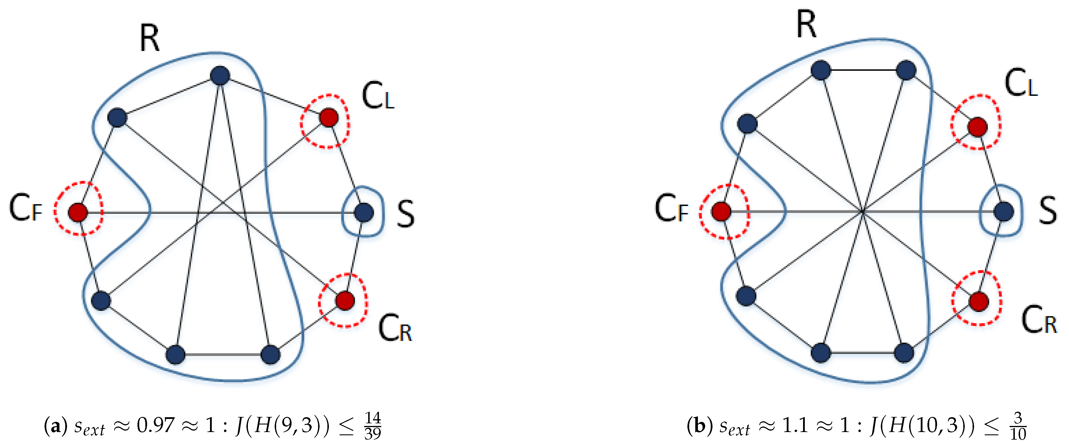
To find an upper bound of tightness for Harary graphs type (c), the results obtained for Harary graphs type (b) can be used because these results were calculated in continuous space. For this purpose, it is enough consider the condition

v_{0} \notin S

. Figure 6 shows an example of the desired component S and cutting vertices

C = {C_{L} \cup C_{R} \cup C_{F}}

for

H (9, 3)

and

H (10, 3)

3. Conclusion

In this work, we sought to analyze the vulnerability of Harary graphs using the tightness metric as the primary parameter. Different methodologies were employed to calculate the tightness values for three distinct types of Harary graphs. The lower and upper bounds of the tightness values for Harary graphs were presented using existing lemmas and theorems, relying on the fact that Harary graphs are Hamiltonian. Additionally, the tightness values were accurately calculated for Harary graphs of type (a). For types (b) and (c), an acceptable upper bound was obtained due to the complexity of the graph structure. Given the novelty of the tightness parameter, there is still limited information available about its properties and applications. This gap in the current understanding presents an opportunity for future research to further explore and expand the knowledge surrounding this graph vulnerability measure.

References

An M. "Harary index, binding number and toughness of graphs", Kuwait Journal of Science, 51, pp. 100176 (2024). [CrossRef]
. [CrossRef]
Baldoni R., Bonomi S., Querzoni L., Piergiovanni S.T. "Investigating the existence and the regularity of logarithmic harary graphs", Theoretical computer science, 410, pp. 2110-2121 (2009). [CrossRef]
Bauer D., Kahl N., Schmeichel E., Woodall D.R., Yatauro M. "Toughness and binding number", Discrete Applied Mathematics, 165, pp. 60-68 (2014). [CrossRef]
Chen Y., Fan D., Lin H. "Factors, spectral radius and toughness in bipartite graphs", Discrete Applied Mathematics, 355, pp. 223-231 (2024). [CrossRef]
Dunkum M., Lanphier D. "Edge integrity of nearest neighbor graphs and separator theorems", Discrete Mathematics, 342, pp. 2664-2679 (2019). [CrossRef]
Fujita S., Furuya M. "Safe number and integrity of graphs", Discrete Applied Mathematics, 247, pp. 398-406 (2018). [CrossRef]
Gu X. "Toughness in pseudo-random graphs", European Journal of Combinatorics, 92, 103255 (2021). [CrossRef]
Harary F. "Graph Theory". Massachusetts: Addison-Wesley Publication Company. Inc. 1st, (1969). [CrossRef]
Javan A., Javan M., Jafarpour M., Moazzami D., Moeini A. "On the J-Tightness of graphs", Journal of Algorithms and Computation. 53, pp. 57-74 (2021). [CrossRef]
Jin Q., Li S., Xie M. "3-path-connectivity of Cayley graphs generated by transposition trees", Discrete Applied Mathematics, 339, pp. 292-299 (2023). [CrossRef]
Katona G. Y., Khan H. "Minimally tough chordal graphs with toughness at most 1/2", Discrete Mathematics, 000, pp. 1-7 (2023). [CrossRef]
Liang J, Liu X., Lou D., Zhang Z.B., Qin Z. "Cyclic edge and cyclic vertex connectivity of (4,5,6)-fullerene graphs", Discrete Applied Mathematics, 351, pp. 94-104 (2024). [CrossRef]
Li F., Zhang X., Broersma H. "A polynomial algorithm for weighted scattering number in interval graphs", Discrete Applied Mathematics, 264, pp. 118-124 (2019). [CrossRef]
Liu Q., Huang X., Zhang Z. "Optimally restricted edge connected elementary Harary graphs". Theoretical Computer Science. 29, pp. 131-138 (2013). [CrossRef]
Li Y., Gu R. "Bounds for scattering number and rupture degree of graphs with genus", Applied Mathematics and Computation, 337, pp. 329-334 (2018). [CrossRef]
Li Y., Shi Y., Gu X. "Spectrum bounds for the scattering number, integrity, tenacity of regular graphs", Future Gen. Comp. Sys., 83, pp. 450-453 (2018). [CrossRef]
Milojevic A. "Connectivity of old and new models of friends-and-strangers graphs", Advances in Applied Mathematics, 155, 102668 (2024). [CrossRef]
Moazzami D. "Tenacity of a graph with maximum connectivity", Discrete Applied Mathematics, 159, pp. 367-380 (2011). [CrossRef]
Park D., Ostuni A., Hayes N., Banerjee A., Wakhare T., Wong W. "The toughness of Kneser graphs", Discrete Mathematics, 334, pp. 112484 (2021). [CrossRef]
Prabhath A., Mathew S., Mordeson J.N. "Generalized cycle connectivity in fuzzy graphs", Fuzzy Sets and Systems, 482, 108909 (2024). [CrossRef]
Song X., Zhang S., Chen X., Gao S. "The algebraic connectivity of barbell graphs", Discrete Mathematics, 347, 114027 (2024). [CrossRef]
Zhou S. "Binding numbers and restricted fractional (g,f)-factors in graphs", Discrete Applied Mathematics, 305, pp. 350-356 (2021). [CrossRef]

Figure 1. Three examples of different types of Harary graphs

Figure 2. Harary graphs type (a) desirable cut

Figure 3. Optimal cut for calculating tightness of H(9,4),

J (H (9, 4)) = 0.5

Figure 3. Optimal cut for calculating tightness of H(9,4),

J (H (9, 4)) = 0.5

Figure 4. Two different cuts for Harary graphs types (b) and (c)

Figure 5. Harary graphs type (b) sample first cut

Figure 6. Two upper bound cuts for Harary graphs types (b) and (c)

Disclaimer/Publisher’s Note: The statements, opinions and data contained in all publications are solely those of the individual author(s) and contributor(s) and not of MDPI and/or the editor(s). MDPI and/or the editor(s) disclaim responsibility for any injury to people or property resulting from any ideas, methods, instructions or products referred to in the content.

© 2024 by the authors. Licensee MDPI, Basel, Switzerland. This article is an open access article distributed under the terms and conditions of the Creative Commons Attribution (CC BY) license (http://creativecommons.org/licenses/by/4.0/).

Copyright: This open access article is published under a Creative Commons CC BY 4.0 license, which permit the free download, distribution, and reuse, provided that the author and preprint are cited in any reuse.

Alerts

MDPI Initiatives

Important Links

Choose an area of interest and we will send you notifications of new preprints at your preferred frequency.

Disclaimer

Tightness of Harary Graphs

Abstract

Keywords:

Subject:

1. Introduction

2. Tightness of Harary Graphs

2.1. Tightness of Harary Graphs Type (a)

2.2. Tightness of Harary Graphs Types (b) and (c)

3. Conclusion

References

MDPI Initiatives

Important Links

Subscribe