1. Introduction
The study of the evolutionary history and relationships among or within groups called phylogenetics. Traditionally phylogenetic inference has relied on models like Maximum Likelihood (ML) and Bayesian inference. While effective these methods need substantial computational power specially with the increasing size of data. Lately the integrating between Machine Learning and phylogenetic analysis has shown promise in addressing these challenges thus enhancing the efficiency and accuracy of phylogenetic tree construction and tree inference.
In phylogenetic analysis features are categorized either as homology or homoplasy. Homology refers to traits received from the common ancestor on other hand homoplasy one describes traits that develop independently, often due to convergent or parallel evolution. Distinguishing between these features is essential for accurate phylogenetic reconstruction. Homologous features indicate shared lineage, whereas homoplasies can obscure these connections if not properly identified. By accurately differentiating these features, researchers can improve the precision of phylogenetic analyses and gain deeper insights into evolutionary history.
Our dataset consists of binary data (0’s and 1’s) forming an matrix, where represents taxa, and represents features. We are particularly interested in exploring n-dimensional aspects, such as finding the best phylogenetic tree using the maximum parsimony criteria.
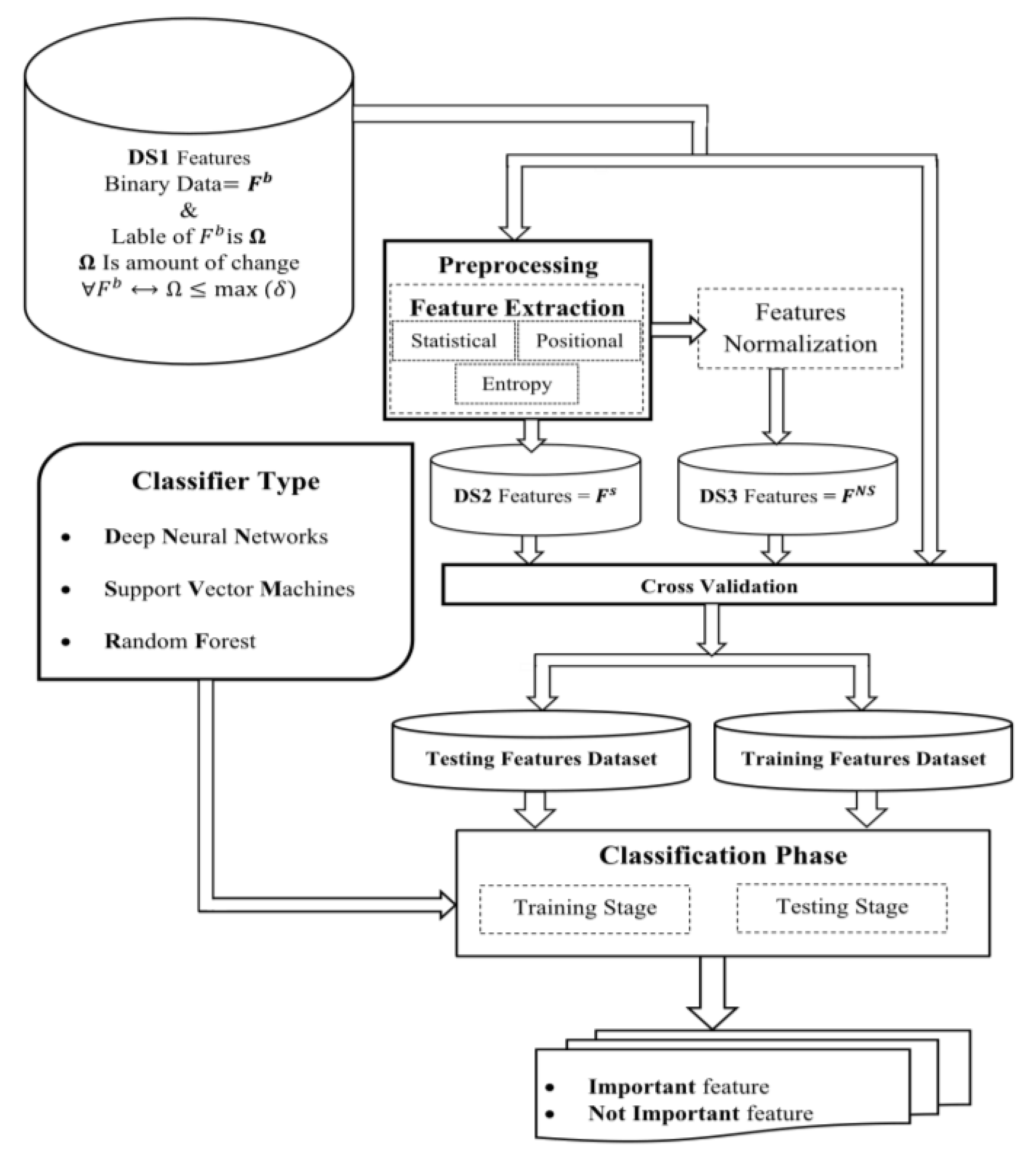
The principal objective of our research is to improve the accuracy and efficiency of phylogenetic tree reconstruction by optimizing feature selection with the help of machine learning models, including Deep Neural Networks (DNN), Support Vector Machines (SVM), and Random Forests (RF). By identifying the most informative features prior to the phylogenetic analysis, we aim to simplify the tree structure and enhance its consistency.
To achieve our research objectives, we propose the following steps
Perform maximum parsimony to extract the phylogenetic tree [
1]
Identify all branches and their ancestral values
Determine the amount of change for each feature
Develop a model to predict feature quality before phylogenetic analysis
1.1. Identify Subgroups and Their Quality
Our research focuses on creating and utilizing a feature selection algorithm to enhance phylogenetic tree reconstruction. Feature selection is inherently challenging, particularly when identifying subgroups of features with a high Consistency Index (CI), which significantly impacts the efficacy of phylogenetic analysis. Our goal is to address these challenges and demonstrate the robustness of our methodology.
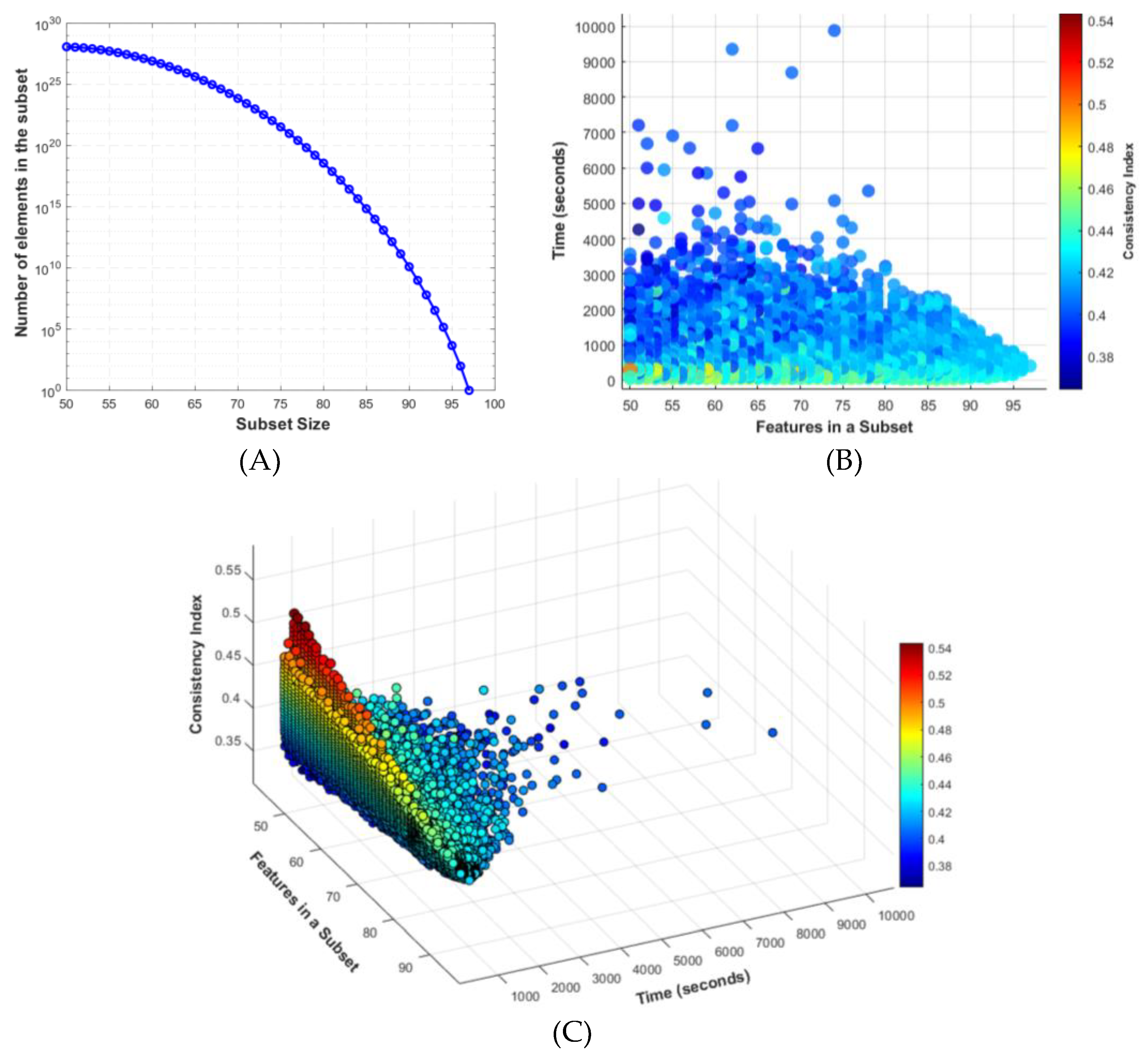
In recent experiments, we highlighted the complexities involved in feature selection. While identifying the most parsimonious tree is crucial, understanding the variability and computational complexity of feature selection is equally important. To explore these challenges, we randomly selected subgroups of features and used the PAUP* program to perform a Branch and Bound search. We recorded search times, feature counts, and CI values, as shown in
Figure 1.
In
Figure 1.A shows the relationship between the number of elements in a subset and the subset size. As the subset size decreases, the number of possible combinations increases exponentially
On the other hand,
Figure 1.B presents a scatter plot of the time taken for the Branch and Bound search relative to the number of features in each subset. The color coded Consistency Index (CI) values illustrate the variability in the data.
Finally,
Figure 1.C offers a 3D plot depicting the relationship between the Consistency Index (CI), the number of features, and the processing time, highlighting the challenge of finding subgroups that balance computational feasibility with high CI values.
These figures collectively underscore the delicate balance required in feature selection for phylogenetic analysis, emphasizing the combinatorial explosion and the variability in search times and CI values as key challenges. This analysis demonstrates the importance of developing robust feature selection methods to improve the accuracy and efficiency of phylogenetic studies.
1.2. Leveraging Machine Learning for Phylogenetic Analysis of Historical Scripts
Systematics has expanded beyond biology into the field of scriptinformatics, which applies evolutionary modeling and computer science to understand the historical evolution of scripts. Scripts are treated similarly to living organisms, enabling a systematic study of their development and cultural dissemination [
2,
3,
4,
5,
6,
7,
8,
9].
Advances in computational methods, particularly in feature selection and machine learning, have significantly enhanced the accuracy of phylogenetic inference. The complexity of high dimensional data in phylogenetics necessitates advanced algorithms to select informative features thereby improving model effectiveness and deepening evolutionary understanding [
3,
4,
5,
7,
8,
9].
Despite these advancements, constructing phylogenetic trees especially calculating Maximum Parsimony scores remains time consuming and costly. Traditional methods often struggle with large, complex datasets creating bottlenecks in evolutionary biology research. Additionally, identifying informative features from large datasets is challenging, as it frequently requires reconstructing trees to evaluate different feature subsets, making the process increasingly impractical as data sizes grow [
10].
Neural network approaches, as demonstrated in previous studies, offer a groundbreaking solution by directly predicting tree lengths from datasets, thereby avoiding exhaustive phylogenetic analysis. This method significantly reduces computational time, eliminating the need for repeated tree construction and scoring, thus streamlining phylogenetic studies [
2,
4].
Although neural network methods simplify feature selection and allow quick assessment of feature impacts on predicted tree lengths, their full potential for handling complex evolutionary scenarios such as feature duplication, loss, and introgression in large-scale phylogenetic analyses remains to be fully explored. These scenarios introduce significant heterogeneity into datasets, which our application aims to address [
11].
In scriptinformatics, scripts are analyzed as pattern systems representing symbolic communication through their symbols, syntax, and layout rules. These systems are defined by binary features that indicate the presence (1) or absence (0) of specific traits, enabling the study of scripts’ evolutionary development. This approach highlights the importance of pattern systems, like Morse code and historical scripts, in the evolution of writing [
4]. A notable example is a review paper that discusses the use of taxonomy in graph neural networks, citing 327 relevant studies to demonstrate the extensive research in this field [
12].
The field of scriptinformatics leverages computational advancements to study the evolution of scripts, viewing them as pattern systems defined by symbols, syntax, and layout rules. This method allows for the examination of the properties and evolutionary paths of scripts, providing a framework to understand the dynamic relationship between writing systems and the societies that develop them [
3,
4,
5,
7,
8,
9].
Given these developments, our research focuses on the evolutionary analysis of historical scripts using optimized feature selection techniques to reconstruct phylogenetic trees of various script variants. We study Arabic, Aramaic, and Middle Iranian scripts to uncover their evolutionary relationships and contribute to the broader field of scriptinformatics. The dataset used in this study is publicly accessible, promoting transparency and encouraging further research in this growing field [
3,
4,
5,
7,
8,
9].
Beyond its contributions to scriptinformatics, our research offers practical applications in archaeology. This method has the long-term potential to gradually unravel script evolution, bringing us closer to deciphering previously undeciphered inscriptions found by archaeologists.
This research explores the evolution of Arabic, Aramaic, and Middle Iranian scripts by analyzing them as distinct pattern systems to reconstruct their phylogenetic trees. We utilize publicly accessible datasets from GitHub [
13]. By uncovering deep evolutionary connections, this study significantly advances the field of scriptinformatics, offering new insights into the historical development of these scripts.
This article is structured as follows: the Background section introduces the use of artificial neural networks in phylogenetic reconstruction; the Methods section describes our approach; the Experimental Results section presents our findings; the Discussion section interprets the results and their implications; and the Conclusions section summarizes the outcomes and suggests future research directions.
4. Experimental Results
The performance of the proposed models DS1 (), DS2 () and DS3 (). The evaluation is presented in terms of Acc means Accuracy, FAR, FRR, AUC and EER
In this study, we analyzed the impact of feature selection on the phylogenetic tree reconstruction using Maximum Parsimony criteria. Our findings are summarized through a series of figures and a table that highlight the distribution of feature changes, the resulting phylogenetic trees, and the consistency index (CI) across different thresholds of feature selection.
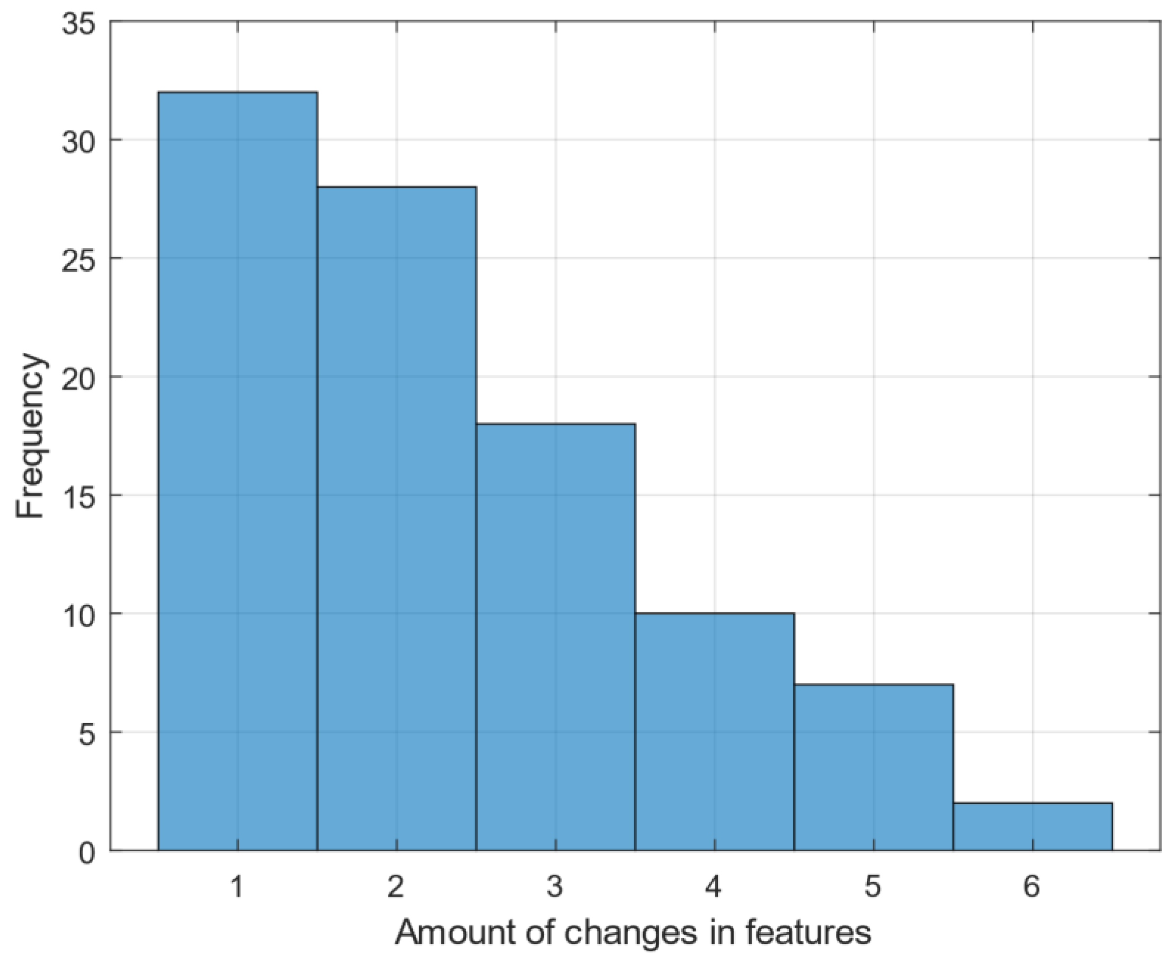
The histogram of
Figure 3 illustrates of features based on the number of changes they induce. The histogram shows that the majority of features cause only one change, with a decreasing number of features causing higher amounts of changes. This distribution is crucial as it underscores the direct relation for reducing the complexity of the phylogenetic tree by focusing on the most impactful features.
The data in
Table 4 highlights the trade-off between the number of features and the phylogenetic tree’s consistency and length. Selecting features that cause fewer changes not only simplifies the tree but also enhances its consistency, as indicated by higher Consistency Index (CI) values.
By focusing on features that cause minimal changes, we produced a phylogenetic tree that is both shorter and more consistent. Specifically, selecting only those features that induce one change results in a cladogram with a tree length equal to the number of features which equal to 32 and a perfect CI of 1.0. This approach significantly improves the efficiency and accuracy of phylogenetic analysis, as evidenced by the simplified tree structure and higher CI values.
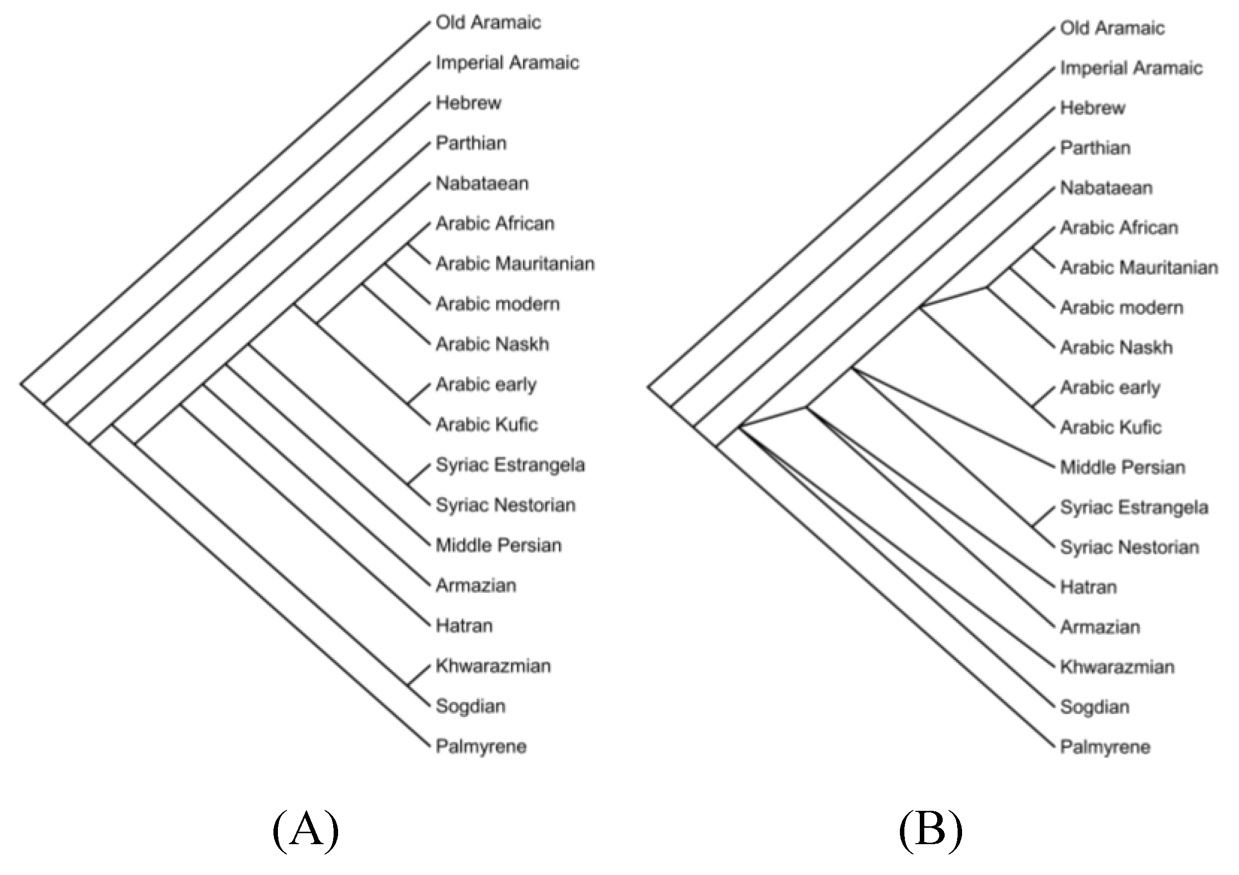
In
Figure 4 two phylogenetic trees are obtained using a Maximum Parsimony search.
Figure 4.A includes all 97 features, resulting in a tree length of 229 and a Consistency Index (CI) of 0.424. In contrast,
Figure 4.B features a subset of features that cause only one change, significantly simplifying the tree structure. This tree has a length equal to the number of features is 32 and achieves a perfect CI of 1.0. This comparison clearly demonstrates that selecting features causing minimal changes leads to a more parsimonious and consistent phylogenetic tree.
Moreover, shows the number of features selected at different δ (threshold) values, along with their corresponding tree lengths and CI values. As δ decreases in (6) fewer features are selected, resulting in shorter tree lengths and higher CI values, which suggest better consistency in the phylogenetic trees.
The table also includes the Optimal tree and Time Sec columns. The Optimal tree column indicates the number of optimal trees found after performing a Branch and Bound search, all having similar maximum parsimony scores. Generally, fewer optimal trees are found as δ decreases, reflecting more stable feature selection. The Time Sec column shows that computation time drops significantly with lower δ values, from 369.3 seconds at δ = 6 to nearly 0 seconds at , highlighting the efficiency gained through feature reduction.
Given that Deep Neural Networks (DNN), Support Vector Machines (SVM), and Random Forests (RF) are nondeterministic algorithms, we performed each test 50 times to ensure the stability and reliability of our results. By averaging the outcomes over these multiple runs, we mitigated the effects of random variation and provided a robust assessment of each model’s performance. This approach ensures that the results presented in the subsequent figures accurately reflect the true performance characteristics of the models across different datasets and folds.
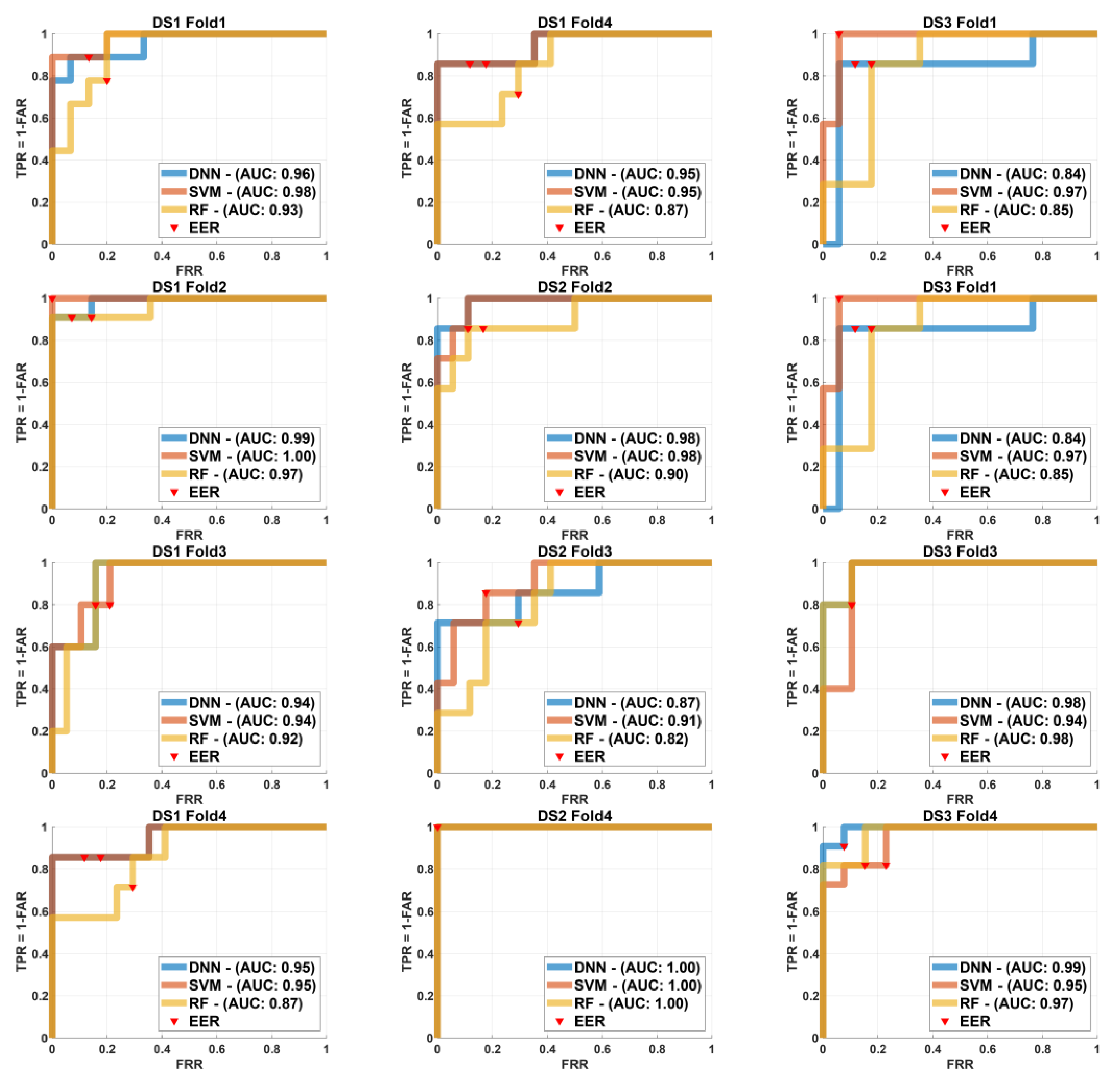
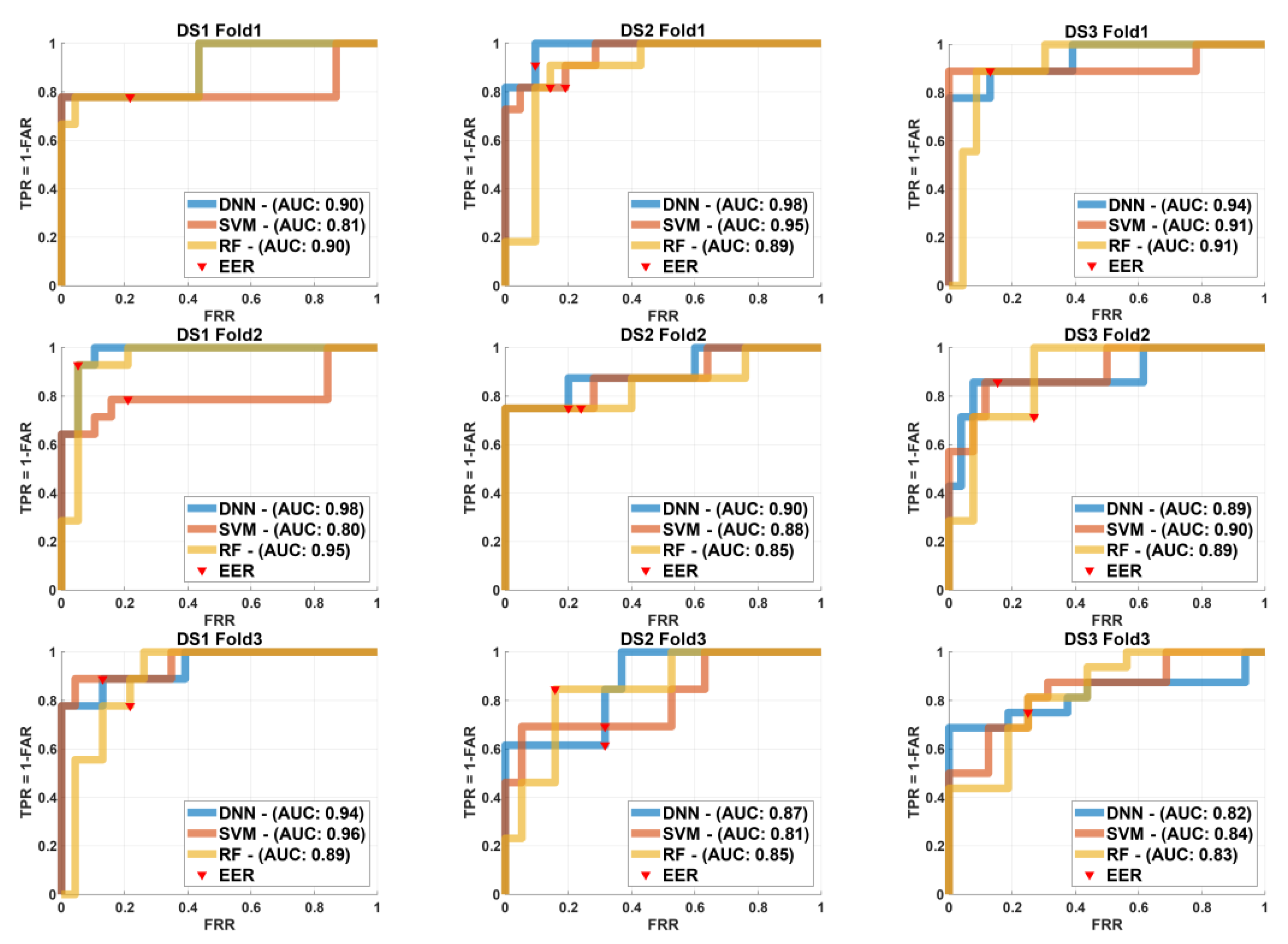
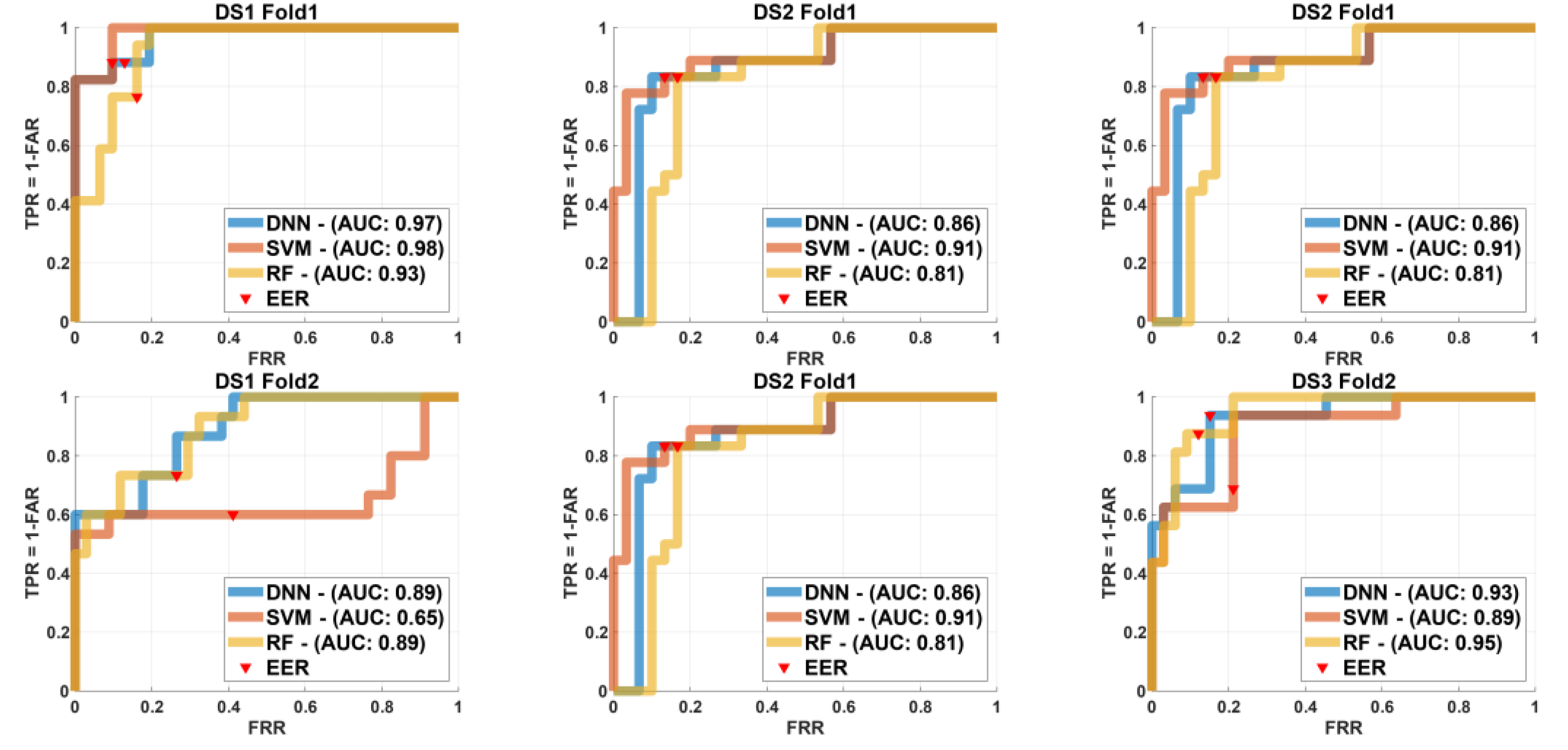
In order to show the effect of different models and sizes for training and testing we use the ROC curve and EER for different k-fold sizes as demonstrated on
Figure 5 to show the tests of k=4 folds,
Figure 6 for k=3 and in case of k=2 is shown in
Figure 7.
In case of k-4 folds=4,
Figure 5 illustrates the ROC curves for the three different machine learning models Deep Neural Network (DNN), Support Vector Machine (SVM), and Random Forest (RF) across four folds (k=4) for each of the three datasets (DS1, DS2, and DS3). Each row in the figure corresponds to a different fold (Fold 1 to Fold 4), and each column corresponds to a different dataset. The ROC curves for each model are plotted, with the Area Under the Curve (AUC) values annotated for comparative performance analysis. Additionally, the Equal Error Rate (EER) locations are marked on each curve.
In
Figure 5 the SVM model demonstrated superior performance for
in Fold 1 with an AUC of 0.98, while all models showed similar performance for
with DNN slightly outperforming others for
. In Fold 2, SVM again outperformed the others for
and
with DNN leading for
. In Fold 3, DNN achieved the highest AUC for
performed similarly well for
, and both DNN and SVM showed equal AUC for
. Finally, in Fold 4 SVM maintained the highest AUC for
while DNN outperformed for
and
. These results highlight the robustness and variable effectiveness of each model across different datasets and folds, underscoring the importance of selecting a model suited to the specific dataset.
Additionally,
Figure 6 presents the ROC curves for the DNN, SVM, and RF models across three folds (k=3) for each of the three datasets (
,
, and
). All row relates to a different fold and each column to a different dataset. The ROC curves are plotted with AUC values marked for comparison and EER locations are marked on each curve for reference.
Fold 1
Figure 6 the DNN outperformed other models for
with
on other hand SVM had the highest AUC for
equal to 0.95 and RF led for
with
. In Fold 2, SVM and RF performed similarly well for
, both achieving an AUC of 0.85. DNN topped for
with an
while RF maintained the lead for
with
. In Fold 3, DNN proven the best performance comes using
with
SVM intended for
with
and RF persisted to perform effectively for
with
.
Moreover,
Figure 7 describes the ROC for DNN, SVM, and RF models across
two folds to each of the three datasets we have
,
, and
. Each row relates to a different fold and each column to different dataset. The ROC curves are plotted alongside AUC values and EER locations are marked on each curve.
Figure 7 particularly Fold 1 the DNN shown the highest performance for
with
whereas SVM displayed better performance in
with
. For
RF held the greatest AUC value
. In Fold 2 DNN to
with
and SVM showed a high performance for
with
. RF continued to perform best for
with
. These results indicate the varying strengths of each model across different datasets and folds highlighting the importance of selecting the most suitable model based on dataset characteristics to achieve ideal performance.
Table 5 presents the average accuracy (Acc), FRR and FAR for the DNN, SVM and RF models across different folds to datasets
,
, and
. This thorough comparison shows the values of each metric demonstrating the efficiency of each model.
Given the non-deterministic characteristics of DNN, SVM, and RF algorithms, there is a possibility of generating slightly different results for each execution using the same data and parameters in our case
,
, and
. To counteract this variability, we carried out 50 iterations of every test and determined. The average results AUC and EER across different fold sizes for the datasets
Table 6 presents these.
The outcomes in
Table 6 show that DNN delivers strong performance across different datasets and fold sizes, with AUC values spanning from
to
and EER values between
and
. Notably DNN reached the highest AUC of
for both
and
at
, highlighting it exceptional predictive ability.
SVM also shown robust performance for and with AUC and at . However, its performance on was somewhat decreased with AUC between , and and EER values from to .
RF displayed more variable performance with AUC ranging from to across datasets. Although RF variability it kept relatively low EER values particularly in where it achieved an AUC of 0.91 and an EER of 0.17 at k=4.
In summary tho all models shown effective performance DNN appeared as overall due to its high AUC values and low EER around all datasets and folds. SVM also performed well, particularly for and , while RF proved reliable though slightly more variable, performance.
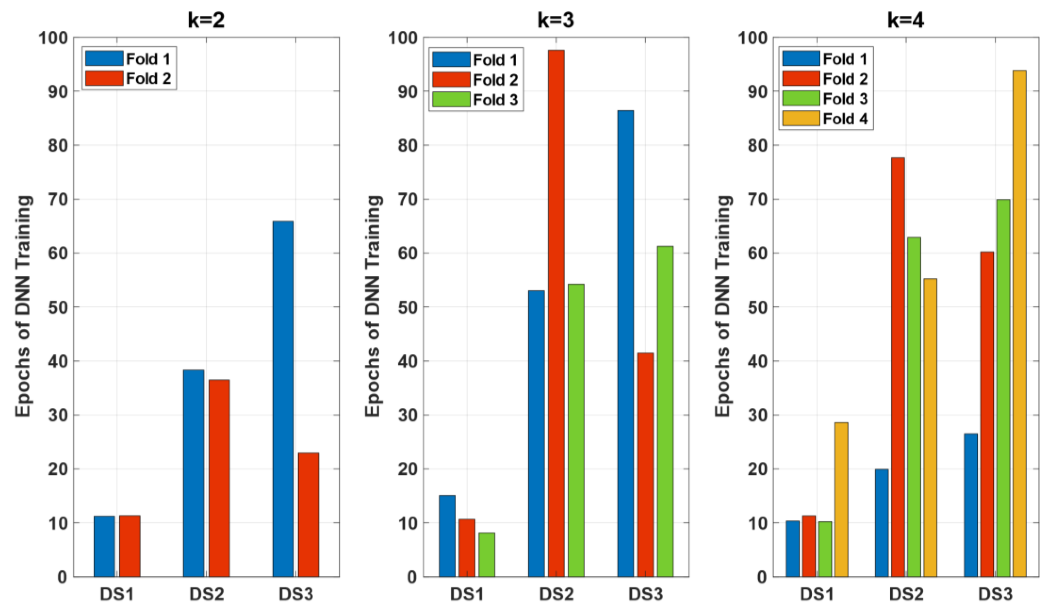
Lastly,
Figure 8 illustrates the number of epochs required for the DNN training across different folds and datasets (
,
,
) for k=2, k=3, and k=4. Each bar represents the number of epochs needed to achieve the final model performance for each fold within the respective k-fold cross-validation setup.
The results indicate that the number of epochs varies significantly across different datasets and folds. For k=2, required the highest number of epochs in both folds, indicating that this dataset posed more complexity for the DNN model to learn effectively. In contrast, required fewer epochs, suggesting it was easier for the model to converge.
When k=3, the variability in the number of epochs increased, particularly for , which again required the most training epochs across all folds, highlighting its complexity. also showed a substantial increase in epochs needed for Fold 2, suggesting variability in the training process.
For k=4, continued to demand a high number of epochs, with Fold 1 showing the maximum epochs among all the datasets and folds. , however, showed more consistency across folds, indicating a more stable training process for this dataset under the k=4 setup.
The analysis shows that consistently required more training epochs across all k values, reflecting its higher complexity and the model’s need for more iterations to learn effectively. generally required fewer epochs, suggesting it was less complex and easier for the DNN to train. This variability in training epochs across datasets and folds underscores the importance of considering dataset complexity and ensuring adequate training to achieve optimal model performance.
5. Discussion
This research examined the influence of feature selection on the reconstruction of phylogenetic trees through machine learning algorithms. The results highlight the essential importance of proficient feature selection in improving both the accuracy and reliability of phylogenetic studies. We applied DNN, SVM and RF to the binary dataset and preprocessed datasets (, and ) assessing and comparing their performance across different fold sizes.
An important observation pertains to the utilization of binary dataset which offers simplicity to easier implementation and faster processing times. However, its general limitation is the different number of input size to machine learning algorithms which restricts its application on different datasets that hold different sizes.
In contrast, using preprocessed features or normalized one leads to additional complexity due to preprocessing steps. However, these offer the flexibility of maintaining a fixed input size letting machine learning models to be applied across datasets of varying sizes. This adaptability is crucial for generalizing models to a broader range of phylogenetic analyses and ensuring robust performance across different scenarios.
Our results indicate that DNN consistently performed well across all datasets and folds, achieving the highest AUC values and maintaining low EER values, particularly for and . This suggests that DNN effectively captures complex patterns within the data, making it a reliable choice.
SVM also demonstrated strong performance, particularly for and , where it achieved high AUC values. However, its slightly lower performance on . This aligns with the known strengths of SVMs, which perform well with well-defined boundaries but may struggle with more complex or noisy data.
RF exhibited more variable performance, with AUC values ranging from 0.82 to 0.91 across the datasets. Although this variability RF maintained relatively low EER values, particularly for . RF’s ability to handle large datasets makes it valuable for identifying key evolutionary traits, even though overall performance was less compared to DNN and SVM.
Our study also highlights the importance of considering dataset complexity consistently required more training epochs in case of DNN across all k values showing its higher complexity and the need for more iterations to achieve effective learning. This highlights the necessity of adequate training to optimize model performance.
Finally, using cross-validation provided a comprehensive assessment of each model’s predictive capability. Because DNN, SVM, and RF are nondeterministic algorithms, each run with the same data and settings can yield slightly different results. To account for this variability we ran each test 50 times and averaged the outcomes. This approach Reduced the effects of random variation and ensured the stability and reliability of our results, providing a more accurate evaluation of each model’s performance.
