Preprint
Article

Transfer Learning and Deep Neural Networks for Robust Intersubject Hand Movement Detection from EEG Signals

Altmetrics

Downloads

78

Views

30

Comments

0

A peer-reviewed article of this preprint also exists.

Submitted:

17 August 2024

Posted:

19 August 2024

You are already at the latest version

Alerts
Abstract
In this proposed work, five systems were developed to classify four motor functions—forward hand movement (FW), grasp (GP), release (RL), and reverse hand movement (RV)—from EEG signals. The dataset used is WAY-EEG-GAL, involving participants performing a sequence of hand movements. During preprocessing, bandpass filtering was applied to remove artifacts and focus on the mu and beta frequency bands. The first system, a preliminary study model, explored the overall framework of EEG signal processing and classification. It utilized time-domain features like variance and frequency-domain features like alpha and beta power, with classification performed using a KNN model. Insights from this system informed the development of a baseline system, which uses the same dataset but different feature extraction and classification paradigms. This baseline system combined the common spatial patterns (CSP) method with continuous wavelet transform (CWT) for feature extraction and employed a GoogLeNet classifier with transfer learning. Classification was performed on six unique pairs of events derived from the four motor functions, using both intrasubject and intersubject methods. The baseline system achieved the highest accuracy of 99.73% for the GP-RV pair and the lowest accuracy of 80.87% for the FW-GP pair in intersubject classification. Building on this, three additional systems were developed to perform 4-way classification. Among these, the final model, ML-CSP-OVR, achieved the highest intersubject classification accuracy of 78.08% using all combined data and 76.39% for leave-one-out intersubject classification. This proposed model, which features a novel combination of CSP-OVR, CWT, and GoogLeNet, demonstrates strong potential as a general system for motor imagery (MI) tasks without being subject-dependent.
Keywords: 
Subject: Engineering  -   Electrical and Electronic Engineering

1. Introduction

A Brain-Computer Interface (BCI) system serves as a bridge between the brain's biophysical signals and external devices that can be controlled using these signals. These signals are typically acquired through methods such as Electroencephalogram (EEG), functional Magnetic Resonance Imaging (fMRI), or Positron Emission Tomography (PET) [1]. The primary motivation behind developing BCI systems is to assist individuals who have lost motor abilities due to spinal injuries or paralysis. By accurately interpreting brain signals, these individuals can potentially regain motor functions using prosthetics. Brain-Computer Interface (BCI) systems are pivotal in bridging the gap between neural signals and external device control, offering a beacon of hope for individuals with motor impairments. These impairments often result from spinal cord injuries, strokes, or neurodegenerative diseases, leading to significant loss of independence and quality of life. BCIs can translate neural activity into commands for prosthetic limbs, wheelchairs, and other assistive technologies, thereby restoring a semblance of mobility and autonomy. One of the key social implications of BCI technology is its potential to drastically improve the quality of life for individuals who have lost their motor abilities. For instance, according to the World Health Organization, around 250,000 to 500,000 people suffer a spinal cord injury each year, many of whom experience permanent disability. BCIs can offer these individuals a new avenue for interaction with their environment, which traditional rehabilitation methods might not provide. Case studies highlight the transformative power of BCIs. In one notable instance, a quadriplegic individual was able to control a robotic arm using only their brain signals, allowing them to perform basic tasks such as drinking and eating independently. Another study demonstrated that stroke patients could use BCIs to regain control of their paralyzed limbs after extensive training and therapy. These examples underscore the practical applications of BCIs and their potential to reintegrate individuals into their daily lives. Moreover, statistical data reinforces the need for such advancements. According to a report by the National Spinal Cord Injury Statistical Center, the lifetime costs for an individual with a high cervical injury can exceed $4 million. BCIs not only promise to improve the quality of life but also offer a cost-effective solution in the long run by reducing the need for continuous care and assistance. In conclusion, the development and application of BCI systems hold significant social value. They provide a lifeline for individuals who have lost motor functions, offering them a path to regain independence and improve their overall quality of life. By incorporating specific case studies and statistical data, the compelling impact of BCI technology becomes evident, highlighting its critical role in modern rehabilitation and assistive technology. This expanded introduction not only discusses the potential benefits of BCI systems for individuals with motor impairments but also includes relevant statistics and case studies to underscore the importance and impact of this technology.
BCI systems hold transformative potential for individuals suffering from severe motor impairments due to conditions like amyotrophic lateral sclerosis (ALS), spinal cord injuries, or stroke. These systems offer a means to regain some level of interaction with the environment, significantly improving their quality of life. Some case studies are explained in detail below.
1. Amyotrophic Lateral Sclerosis (ALS)
One of the most prominent examples of BCI application is in patients with ALS, a progressive neurodegenerative disease that leads to the loss of motor functions. A famous case is that of Stephen Hawking, who, despite severe disability, communicated and wrote books using a computerized speech synthesis system. Modern BCIs can further enhance such capabilities, allowing for direct brain-to-computer communication without the need for physical input. According to the ALS Association, approximately 5,000 people in the United States are diagnosed with ALS each year. The average life expectancy of a person with ALS is 2-5 years from the time of diagnosis, emphasizing the urgent need for assistive technologies like BCI to maintain communication abilities as motor functions decline.
2. Spinal Cord Injuries
Consider a study conducted by the University of Pittsburgh, where a patient with quadriplegia (complete paralysis) was able to control a robotic arm using a BCI to perform tasks like feeding themselves. This represents a significant breakthrough in assistive technology, as it allows individuals with no motor control to regain a level of autonomy. The World Health Organization estimates that between 250,000 and 500,000 people suffer spinal cord injuries each year, with many losing the ability to move and requiring lifelong care. BCIs could drastically reduce the burden on caregivers by enabling greater independence.
3. Stroke Rehabilitation
BCI systems have also been used in stroke rehabilitation. For example, the work of researchers at the University of Tübingen in Germany showed that stroke patients who used a BCI to control a virtual hand saw improvements in motor function. This approach leverages neuroplasticity, helping the brain to rewire itself and restore lost capabilities. The American Stroke Association reports that about 800,000 people in the United States have a stroke each year. Approximately 50% of stroke survivors experience some form of motor impairment, underlining the potential impact of BCIs in rehabilitation.
EEG is a popular technique for acquiring neural signals because it is non-invasive and offers high temporal resolution. EEG neural signals can be categorized by frequency into delta (0.5-4 Hz), theta (4-8 Hz), alpha (8-12 Hz), beta (12-30 Hz), and gamma (30-100 Hz) bands [2,3]. Motor imagery (MI) or motor activities primarily activate the brain's sensorimotor cortex, leading to sensory motor rhythms (SMRs). These rhythms can be classified using event-related synchronization (ERS) and event-related desynchronization (ERD), which are particularly useful for distinguishing between left- and right-hand movements [4]. Decoding EEG signals involves several steps, starting with preprocessing to remove artifacts such as muscle noise, heart signals (ECG), and ocular movements. Given the non-stationary nature of EEG signals, effective feature extraction techniques like wavelet transformation are essential [3]. Classification of these features can be performed with or without machine learning models. Various artificial neural networks, including convolutional neural networks (CNN), recurrent neural networks (RNN), and recurrent convolutional neural networks (RCNN), have been successfully employed to classify different events of interest from EEG signals [5]. This project aims to develop a system that utilizes robust feature extraction techniques and machine learning classifiers to accurately classify hand movements. Achieving this goal would significantly contribute to the field of BCI, especially benefiting individuals who rely on brain-computer interface prosthetics.

2. Literature Review

During the research for this literature review, it was observed that most studies focus on motor imagery (MI) data rather than actual movement data. However, the techniques used with MI can be applicable to actual movement EEG data since MI activates similar brain areas and preserves the same temporal characteristics [6]. Therefore, this section discusses papers using both MI and actual movement data. Decades of research have gone into developing EEG-based BCI systems since Dr. Hans Berger first recorded EEG signals from humans in the 1930s [7]. Despite this extensive research, a universally reliable system has yet to be developed. The primary challenge is the highly non-stationary nature of brain signals, which are prone to contamination by artifacts such as eye movements, heartbeat signals (ECG), and electrical noise. Additionally, these signals are subject-dependent and vary across different trials, making it difficult to classify even between two movement activities from EEG signals. The difficulty increases with multiclass systems [8]. To overcome these challenges, several techniques have been developed. One popular and efficient technique is Common Spatial Patterns (CSP), which was initially developed to distinguish between two classes [9,10]. The CSP algorithm finds spatial filters that maximize the variance of the filtered signal under one condition while minimizing it under the other condition [11]. Paired with an 8-30 Hz broadband filter, CSP has achieved accuracies of 84-94% in discriminating three actions: left hand movement, right hand movement, and right foot movement within three subjects. An extension of CSP, using pairwise classification and majority voting, has also been described to enable multiclass classification [9]. Other extensions include CSP One-Vs-Rest (OVR), which computes spatial patterns for each class against all others [12,13], and CSP Divide-And-Conquer (DC), which adopts a tree-based classifier approach [13]. Since the effectiveness of CSP generally relies on optimal participant-specific frequency, it is nearly impossible to obtain spatial filters that generalize for optimal discrimination of classes for every person. Several approaches have been employed to address this issue [13,14]. Filter Bank Common Spatial Patterns (FBCSP), which autonomously selects the subject-specific frequency range for bandpass filtering of EEG signals [13]; non-conventional FBCSP, which differentiates classes using a fixed set of four frequency bands, reducing the computational cost [8]; and sliding window discriminative CSP (SWDCSP), which uses a sliding window of overlapping frequencies to filter the EEG signals [15].This paper proposes a model using CSP OVR and CNN with the WAY-EEG-GAL data-set to distinguish four hand movements. Some closely related papers are explored. In [16], the BCI competition III dataset 3a was used, where each subject performs four different motor imagery tasks (left hand, right hand, foot, tongue). Forty-three channels were used out of sixty-four available. CSP was applied with five filters ranging from 8 Hz to 28 Hz, with increments of 4 Hz. A convolutional neural network (CNN) was used as a classifier, with 80% of the data for training and 20% for validation, resulting in a validation accuracy of 93.75% for intersubject classification using combined data. The author of [17] used the WAY-EEG-GAL dataset, where twelve participants performed continuous movements of a single limb to grasp and lift an object. From these continuous movements, six segments of interest (hand start movement, grasp, lift, hold, replace, release) were selected for classification. CSP performed six binary classifications on the pairs formed from the six segments. Continuous wavelets transform (CWT) generated scalograms, which were inputs for the CNN network. The classification used was intersubject classification without leave-one-out. The highest accuracy was for the 'hold' segment at 96.1%, and the lowest was for 'replace' at 92.9%. In [18], the BCI competition IV Dataset 2a was used, where nine subjects performed motor imagery on four movements: left hand, right hand, feet, and tongue. Feature extraction was performed using time-frequency CSP, while Linear Discriminant Analysis (LDA), naïve Bayes, and Support Vector Machine (SVM) were used as classifiers. The results showed that the average computation time was 37.22% less than FBCSP, used by the first winner of BCI competition IV, and 4.98% longer than the conventional CSP method. Li and Feng [19] used the WAY-EEG-GAL dataset for six-movement classification, involving HandStart, FirstDigitTouch, BothStartLoadPhase, LiftOff, Replace, and BothReleased. A random forest algorithm identified the important electrodes from the thirty-two available. Wavelet transform extracted features, which were inputs for the CNN classifier. This model achieved an accuracy rate of 93.22%. For a more comprehensive view of EEG classification techniques used in the past decade, consider other methods besides CSP. In [20], a public BCI Research database from NUST (National University of Sciences and Technology, Pakistan) was used. Eight channels (F3, Fz, C3, Cz, C4, Pz, O1, O2) were selected. Classification of EEG to identify left and right arm movements was conducted using wavelet transformation (WT) and a multilayer perceptron neural network (MPNN or MLP), achieving 88.72% accuracy. Alomari et al. [21] created a publicly available dataset at physionet.org. Eight channels (FC3, FCz, FC4, C3, C1, CZ, C2, C4) were used of the sixty-four available. A bandpass filter from 0.5 Hz to 90 Hz and a notch filter to remove 50 Hz line noise were applied. Independent Component Analysis (ICA) filtered out artifacts. MATLAB's neural networks toolbox built a neural network (NN) with 1-20 hidden layers, and 'MySVM' software performed SVM classification. Classification accuracies were 89.8% using NN and 97.1% using SVM for left- and right-hand movements. In [22], EEG data were obtained from a 26-year-old male moving his right hand. Four channels (AF3, F7, F3, and FC5) were used. The EEG signals were preprocessed using a Butterworth band-pass filter (0.5-45 Hz). Feature extraction was performed using WT, Fast Fourier Transform (FFT), and Principal Component Analysis (PCA). Classification was done using MPNN to classify three movements: open arm, close arm, and close hand. The model, with one hidden layer, ten neurons, and 500 epochs, achieved classification performances of 91.1%, 86.7%, and 85.6% using the three feature extraction methods, respectively. The author of [23] created a custom dataset involving two subjects performing motor imagery of three different right-hand grasp movements. From twenty-four electrodes, the best combination was found using the Genetic Algorithm (GA), based on evolution and natural genetics. Preprocessing involved ICA and a Butterworth High Pass Filter with a 1 Hz cutoff frequency. Features included maximum mu-power, beta-power, and frequencies of maximum mu and beta power. Among the four NN classifiers, Probabilistic Neural Network (PNN) achieved the best classification accuracy at 61.96%. In [24], a public data-set from fifteen subjects performing six functional movements of a single limb (forearm pronation/supination, hand open/close, and elbow flexion/extension) was used. EEGLAB filtered out irrelevant channels, and ICA identified eye and muscle artifacts. A bandpass filter (8-30 Hz) was applied. PCA standardized and reduced data dimensionality. Wavelet Packet Decomposition (WPD) extracted features, providing a multi-level time-frequency decomposition with good time localization. Classification was performed using a Wavelet Neural Network (WNN), typically comprising three layers: input, hidden, and output. This model achieved an intersubject classification accuracy of 86.27% for the six limb movements [24,25]. The field of EEG signal processing has witnessed significant progress in recent years, particularly in feature extraction and classification techniques, driven by the demand for more accurate and real-time applications in areas such as brain-computer interfaces (BCIs), healthcare, and neuroscience research [51,52,53,54]. One of the recent trends is the application of deep learning methods in EEG signal processing. Convolutional Neural Networks (CNNs) have gained popularity due to their ability to automatically extract features from raw EEG data without the need for manual feature engineering [55,56,57,58]. For instance, CNNs have been successfully employed to decode motor imagery tasks in BCIs, leading to improved classification accuracies. Additionally, hybrid models combining CNNs with other deep learning architectures, such as Long Short-Term Memory (LSTM) networks, have been explored to capture both spatial and temporal features of EEG signals, further enhancing performance. Another promising approach involves the use of transfer learning [59,60], which leverages pre-trained models on large datasets to improve the generalization of EEG classification models on smaller, domain-specific datasets. This is particularly useful in the context of EEG, where obtaining large, labeled datasets is challenging. Transfer learning has shown potential in tasks such as emotion recognition and mental workload estimation, where it helps in reducing training time and improving model accuracy. In feature extraction, the fusion of traditional methods like Wavelet Transform (WT) with advanced machine learning techniques has been explored to enhance the representation of EEG signals. For example, continuous wavelet transform (CWT) has been used to capture both time and frequency domain features, which are then classified using machine learning models like Support Vector Machines (SVMs) or Random Forests. Additionally, methods such as Empirical Mode Decomposition (EMD) have been combined with deep learning models to extract intrinsic mode functions that are more representative of the underlying brain activity. Finally, recent studies have also focused on improving the interpretability of EEG classification models. Explainable AI (XAI) techniques are being integrated into EEG processing pipelines to provide insights into how models make decisions, which is crucial for applications in clinical settings. This not only enhances the trustworthiness of the models but also aids in the discovery of novel neurophysiological patterns.

3. Methodology

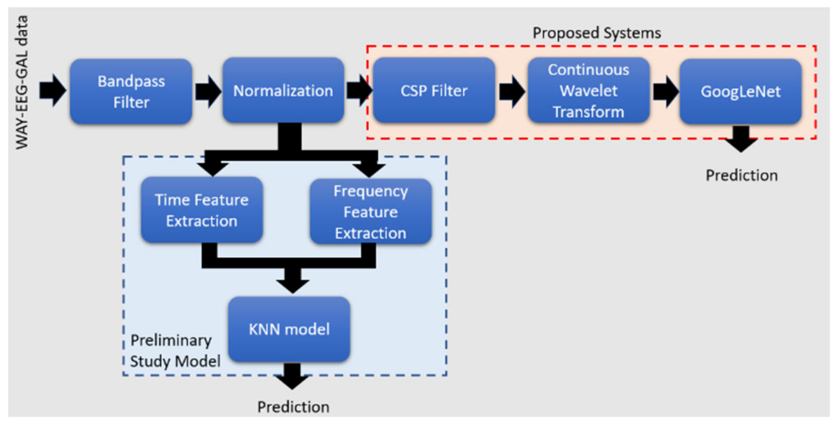
The proposed models in this paper (Figure 1) utilize a combination of CSP filtering, CWT, and GoogLeNet classification. We employed the Common Spatial Patterns (CSP) filter, Continuous Wavelet Transform (CWT), and GoogLeNet classifier for their respective strengths in handling EEG signal classification. CSP is particularly effective for binary classification, enhancing discriminative power by maximizing variance differences between classes. CWT was chosen for its ability to analyze non-stationary signals, capturing both temporal and frequency information crucial for understanding EEG dynamics during motor tasks. By transforming signals into scalograms, CWT preserves important features across different time scales for deep learning models. GoogLeNet, a deep convolutional neural network, was utilized for its robust feature learning and classification capabilities. Leveraging transfer learning, GoogLeNet enhances performance even with smaller datasets by using pre-trained weights from large datasets, improving generalization across subjects and tasks. This combination addresses EEG classification challenges, such as non-stationarity and subject variability, demonstrating high accuracy in binary and multiclass tasks, making it a robust choice for developing reliable BCI systems for motor imagery and hand movement detection. I have provided an expanded introduction of the applied methods with more detailed explanations for CSP filtering, Continuous Wavelet Transform (CWT), and the GoogLeNet classifier as shown below.
Common Spatial Pattern (CSP) Filtering
Common Spatial Pattern (CSP) is a feature extraction technique widely used in the analysis of EEG signals, particularly for classifying motor imagery tasks. CSP works by finding spatial filters that maximize the variance of the signal for one class while minimizing it for the other. This makes it highly effective for distinguishing between different mental states or movements. The CSP algorithm begins by computing the covariance matrices of the EEG signals for each class. These matrices are then averaged and decomposed using eigenvalue decomposition to find spatial filters that create new signals with optimal variance separation between the classes. The filtered signals highlight the most discriminative features for classification. In this research, CSP filters were applied to the EEG signals to enhance the differences between various hand movements (e.g., forward movement vs. grasp). The filtered signals serve as the basis for subsequent feature extraction and classification processes.
Continuous Wavelet Transform (CWT)
Continuous Wavelet Transform (CWT) is a powerful tool for analysing non-stationary signals like EEG. Unlike Fourier transform, which only provides frequency information, CWT offers both time and frequency localization, making it ideal for capturing transient features in EEG data. CWT transforms the EEG signals into a time-frequency domain using wavelets, which are functions that can be scaled and translated. The analytic Morse wavelet, known for its good time-frequency localization properties, was chosen for this transformation. The result is a set of wavelet coefficients that represent the signal's frequency content at different times. These coefficients are then used to generate scalograms—visual representations of the time-frequency characteristics of the EEG signals. Scalograms effectively capture the temporal dynamics and frequency information of the EEG, which are crucial for distinguishing between different motor tasks.

GoogLeNet Classifier

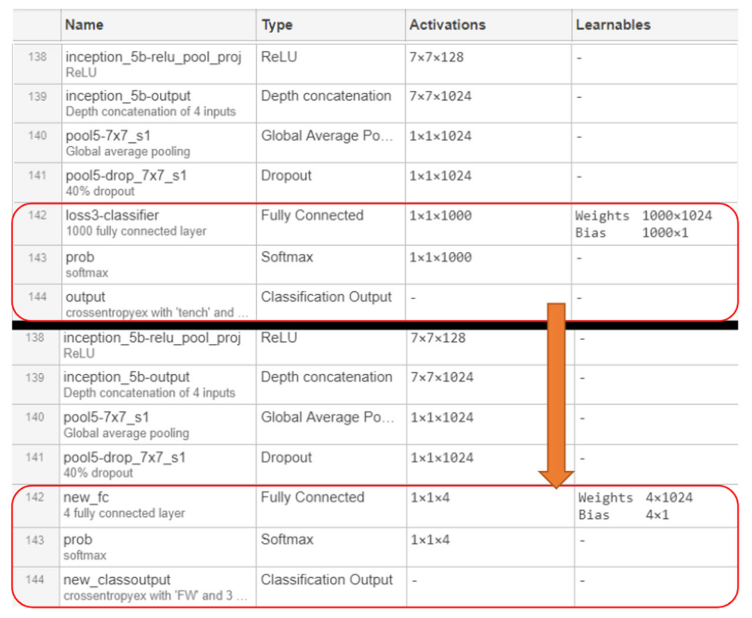
GoogLeNet, also known as Inception-v1, is a deep convolutional neural network that has shown exceptional performance in various image classification tasks. Its architecture consists of multiple convolutional layers that learn hierarchical features from the input data. In this research, the scalograms generated from the CWT are used as input images for the GoogLeNet classifier. To leverage the power of deep learning without requiring extensive training data, transfer learning is employed. The pre-trained GoogLeNet model, initially trained on large image datasets, is fine-tuned by modifying the last two layers to adapt to the specific task of classifying hand movements from EEG signals. This approach significantly reduces the computational cost and training time while improving the model's ability to generalize across different subjects and tasks. By focusing on the most relevant features learned during pre-training, the GoogLeNet classifier achieves high accuracy in distinguishing between the various motor functions.
The integrated use of CSP, CWT, and GoogLeNet forms a robust pipeline for EEG signal classification. CSP enhances discriminative features, CWT captures essential time-frequency information, and GoogLeNet provides powerful classification capabilities. The proposed system demonstrated outstanding performance, achieving high classification accuracies across different motor tasks and subjects, thus highlighting its potential as a general and reliable solution for motor imagery (MI) tasks.
Prior to developing the final model, a baseline system was constructed based on the methods described in [17], as the same dataset was used, achieving classification results exceeding 90%. Additionally, a preliminary study model was created to provide a clear overview of the expectations for developing EEG classification models. Although the baseline system employs CSP as mentioned in [17], the feature extraction using CSP and CWT to produce scalograms differs from the approach used in the referenced paper. These differences are detailed in Section 4.5. The baseline model differentiates the four hand movements in a pairwise manner, functioning as a binary classifier. However, further improvements were made to the baseline model to modify the binary classification into a four-way classification in the last three models. In the preliminary study, time and frequency features were extracted from the EEG signals and fed into a KNN classifier. The extracted time features included mean, variance, skewness, kurtosis, and area under the signal. The extracted frequency features comprised the power of alpha and beta frequency bands. The last three models (ML Model 1, ML Model 2, and ML-CSP-OVR) were developed based on the baseline model with some modifications. The first two variants, ML Model 1 and ML Model 2, introduce a novel classification technique using multiple stages of SoftMax outputs. The final variant, ML-CSP-OVR, employs a novel combination of CSP OVR (One Versus Rest), CWT, and GoogLeNet for multiclass classification.
From the data-set, 4 segments of data corresponding to the 4 events/classes of actions (forward hand movement, grasp, release and reverse) are extracted for classification. These 4 segments or motor actions are shown in Table 1.
In the preliminary study, the 4 events of interest are grouped into two pairs: event 1 and 4, and event 2 and 3 since these pairs involve opposite motor actions. This is grouped under the assumption that the opposite nature involved within these pairs contribute to more accurate classification due to their distinction. For the baseline system, 6 unique pairs, formed from the 4 classes of motor movement, are used for classification. The rest of the models extends the baseline classification to do 4-way classification without using pairs of two.
Table 2. Six pairs for classification in the baseline system.
# # Pairs of classes
1 1 FW-GP
2 2 FW-RL
3 3 FW-RV
4 4 GP-RL
5 5 GP-RV
6 6 RV-RL
These are made in pairs of 2 because CSP was developed for separating two classes of data [9].

4.1. The Dataset

The dataset used in this study is the publicly available WAY-EEG-GAL dataset [42]. It involves twelve participants performing grasp and lift actions across a total of 3936 trials distributed over 10 series. Each participant conducted 328 trials. During the trials, an LED cue signaled the participants to reach for an object, grasp it, and lift it up. The LED turning off indicated the participants to return the object to its original position and retract their hand. The EEG signals were recorded using 32 channels, as depicted in Figure 2. These signals were sampled at 500 Hz. Two types of datasets were provided: holistic and windowed. The windowed dataset was utilized in this study, where the lifting series were segmented into intervals around each lift action. Each window starts precisely two seconds before the LED turns on and concludes three seconds after the LED turns off.

4.2. Data checking and cleaning

Firstly, the dataset was reviewed to verify the information provided in the paper. According to the data-set description, the 12 participants performed a total of 10 series, comprising 28 grasp and lift (GAL) trials for mixed series and 34 trials for each of the other series types. These series include weight, surface, and mixed types. In the weight series, participants interacted with objects of varying weights across three different levels. Meanwhile, the surface series involved objects with different materials on their surfaces. The mixed series combined elements from both the weight and surface series. Figure 3 illustrates these series types for participant 1.
In the selected windowed dataset, the 10th series, which pertains to weight variations, is exclusively available in the holistic data-set. Therefore, for the windowed dataset, only 9 series are accessible. Given that each participant is limited to 2 mixed series, the total number of trials can be calculated as follows:
12 participants × 8 series × 34 trials per series + 12 participants × 2 mixed series × 28 trials per series = 3936 trials
The results align with those reported in the paper. To standardize the data across all series, trials exceeding 28 were discarded, reducing variability and facilitating data processing. Subsequently, each trial's window, starting 2 seconds before the LED activates and ending 3 seconds after deactivation [40], was scrutinized. Plots (Figure 10) were generated for all trials to allow for manual inspection if necessary. A simple code (Listing 1) was employed to verify the 3-second duration; checking the 2-second duration was deemed unnecessary since the LED On duration in the time dataset consistently provided this information. The code was designed to print participant, series, and trial details if deviations from the specified 3-second duration were identified in the trial data, as outlined in the paper.
The code generates several trials all related to participant 7. Therefore, participant 7 is discarded. Therefore, 11 participants, 9 series and 28 trials are used in this study.
Listing 1. A simple check for 3 second duration.
Preprints 115483 i006
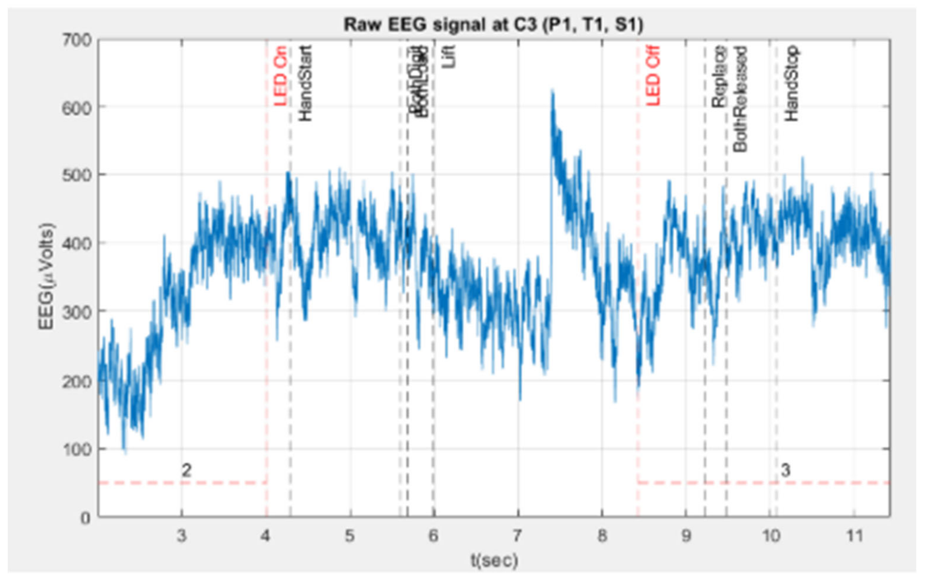
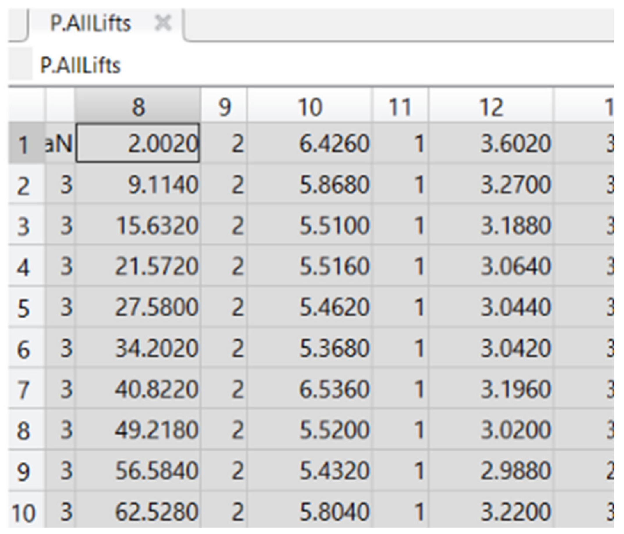
The vertical dashed lines in Figure 4 are drawn to make sense of the time information given in P.AllLifts data (Figure 5). LED On and LED Off times plotted on the graph are calculated by these formulae:
  • LED On time = trial_start_time + LEDon, and LED Off time = trial_start_time + LEDoff respectively. The LEDon and LEDoff used in the calculation are from ws.win. The trial_start_time is also given in ws.win data.
  • x Handstart, FirstDigit, BothLoad, Lift, Replace, BothReleased and HandStop are all calculated in the same way, i.e. summing up the trial_start_time and the respective given time for the actions given in P.AllLifts.
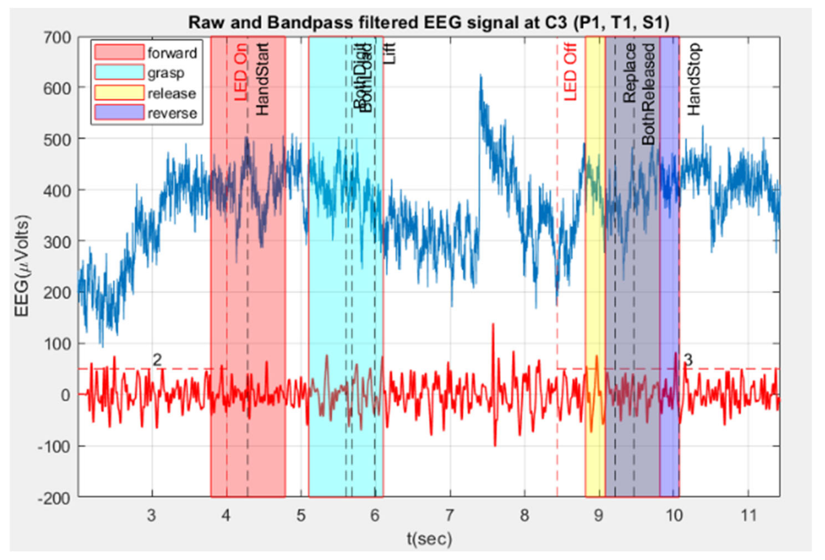
In Figure 6, the blue signal represents the raw EEG signal, while the red signal represents the filtered EEG signal. Four 1-second patches or segments, potentially containing the events of interest, are highlighted. These segments are extracted from the filtered signal for feature extraction, with the filtering process detailed in Section 4.3, Data Preprocessing. The extracted data is then verified to ensure each segment is exactly 1 second or 500 samples in length. Given that the imaging period should not exceed 0.5 seconds [24], a 1-second segment duration is chosen to provide sufficient coverage for the event of interest.
The hand forward reaching movement segment (red patch) is taken around the time when the hand starts moving (HandStart), as this moment likely corresponds to the initiation of the thought to move the hand forward. The grasp segment (cyan patch) is selected at the point when both digits (thumb and forefinger) establish contact with the object. The release segment (yellow patch) is positioned immediately after the Replace action, where the object is returned to its original position. The backward/reverse segment (purple patch) is taken from 1 second before the Handstop point, when the digits separate from the object. Initially, the BothDigit point was used for the grasp segment. Previously, the segment was around BothLoad (when both fingers start applying force to the object). However, due to outliers found in P. AllLifts for certain trials, the BothDigit point is now used instead. In some trials, the reverse segment was cut off, not having the full 1 second length or 500 samples. This issue arose because the reference point was at BothReleased, which, in some trials, is near the end of the trial and thus lacked enough data points for 1 second. This problem was resolved by changing the reference point to the Hand-stop point.

4.3. Data Preprocessing

16 electrodes out of 32 were selected from channels 11-26. These channels are close to the three channels of interest associated with motor movements: C3, Cz, and C4 [41]. A Butterworth bandpass filter with a passband range between 7 and 30 Hz was applied, as motor movements primarily involve sensory motor signals within the mu and beta bands [10]. The Butterworth filter was chosen for its ability to provide a smooth passband output. This filtering process also removes unwanted artifacts such as powerline interference, ocular artifacts, electrocardiogram (ECG), and electromyogram (EMG) signals [17,28]. Z-score normalization was then applied by subtracting the mean and dividing by the standard deviation. In this Section, 5 models built for the classification are described. As mentioned at the start of this Section (Section 4), these 5 systems are as follows: preliminary study model, baseline system, ML model 1, 2, and ML-CSP-OVR.

4.4. Preliminary Study Mode

The objective of the preliminary study is to understand the procedures involved in the EEG signal classification process using machine learning algorithm. Time and frequency features are extracted and used for classification. The features are extracted in MATLAB and exported to Jupyter Lab for KNN classification.
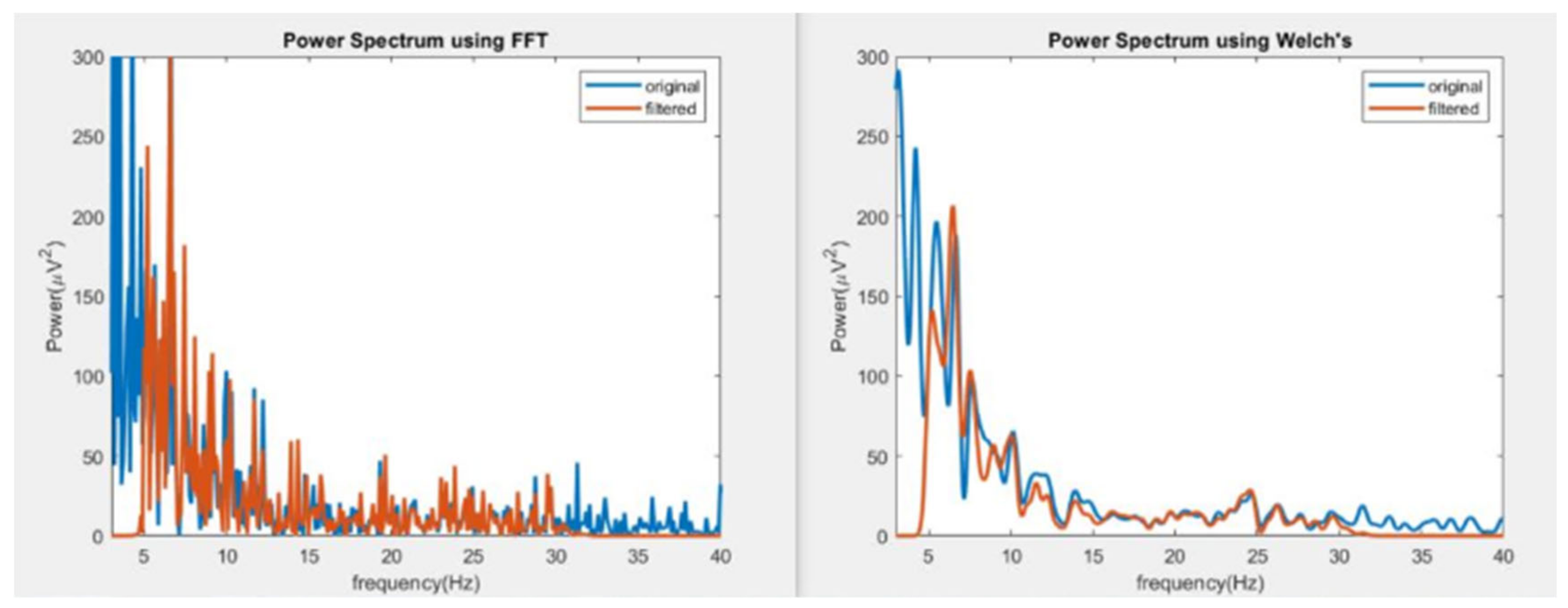
Time features, excluding the zero crossing and peak to peak features, are extracted from the filtered EEG signals. Frequency features such as average powers of beta and alpha frequency bands are extracted by using Welch's method rather than Fast Fourier Transform (FFT) since it produces smoother results due to its averaging method than FFT (Figure 7). The Welch's method is also more robust against non-stationary signals like EEG.
All the extracted features are exported from MATLAB into python compatible data type so that classification can be performed using K Nearest Neighbor classifier (KNN). The first 10 extracted features for event 1 can be seen in Table 3.
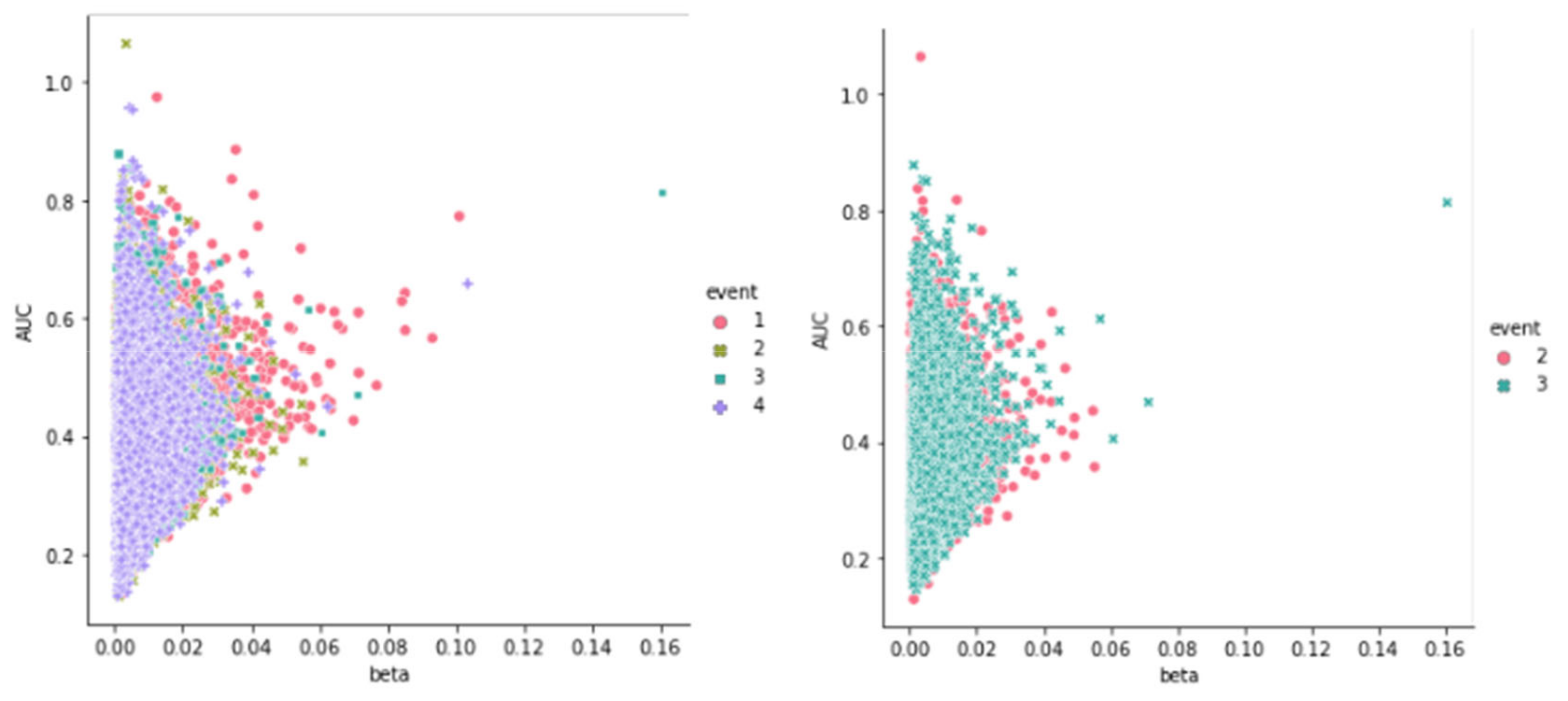
Before the classification is performed, the feature data-set is visualized with the help of scatter plots. Figure 8 shows one such visualization. The features of the events can be observed as closely associated with one another, meaning it will be troublesome for the KNN model to do the classification, even between 2 events. The result of this is discussed further in Section 5.1 below.
Since the data of events are very similar, the classification result is expected to be quite low unless the distribution of the data can be separated. KNN classification works by finding the nearest k neighbors from the data point of interest and taking the mean of those points to get the prediction for the data point. The classification of the algorithm performs best at k = 3.

4.5. The baseline system

The baseline system is built to establish a deep understanding of some of the popular methods used in EEG signal processing using machine learning. Since the techniques are based upon [17], the results can be compared against the ones presented in the paper to see how well the baseline system performs. However, direct comparison is not possible due to different paradigms used; the difference manifested because of the bizarre ways the authors applied their techniques in [17]. An effort was made to understand by contacting the main author of the paper but only to receive a reply that is not satisfactory. One reason is because the author does not clearly remember the methods in the research as it has been 2 years since the research was conducted. Below are the some of the unusual points found in the paper:
i.
the unfiltered data of the 6 selected electrodes have more data points than it is provided in the dataset.
ii.
the CSP method seems to be used on a single electrode.
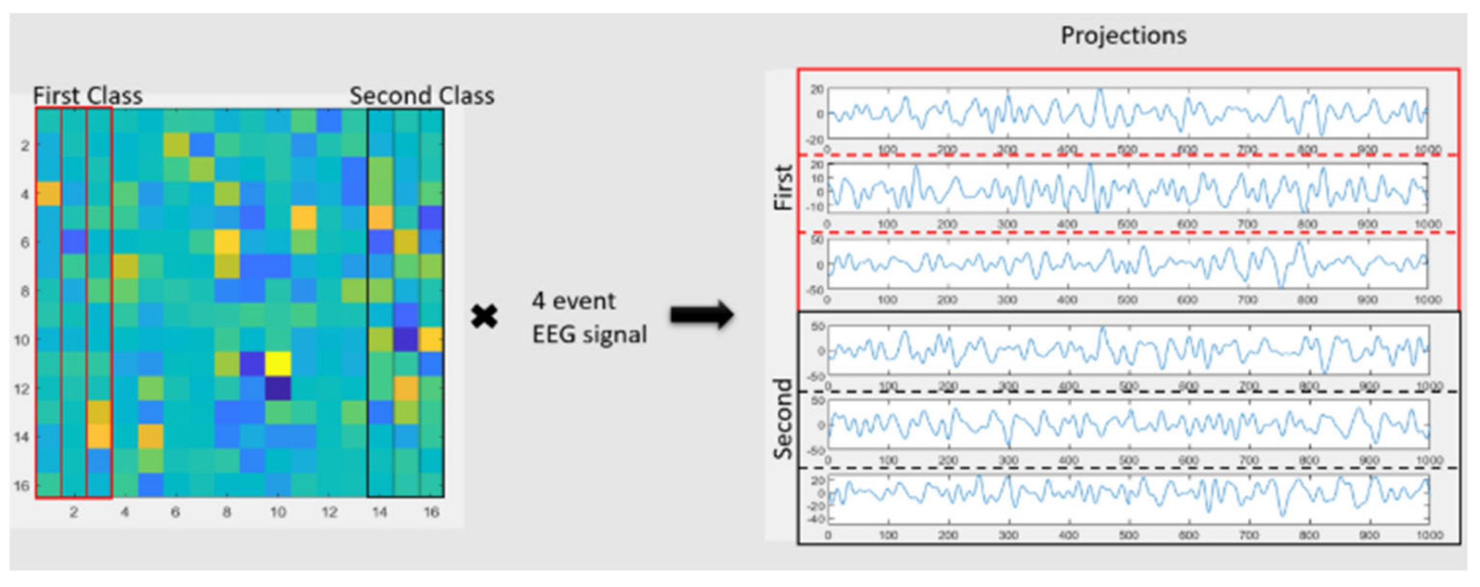
The problem with point (ii) is that CSP is a general eigen decomposition method that finds a weighting of channels, which maximizes the signal to noise ratio [44]. With a single channel or electrode, it would not be necessary to find a set of weights. Therefore, a CSP system was built following closely on the original method (Section 3.1.6). 6 spatial filters were selected (3 for each class for binary classification) because of the need to create RGB images that serve as inputs for the CNN classifier. Common Spatial Patterns (CSP) is a technique used to distinguish between two classes or conditions in EEG signal processing. This method requires the data for the two classes to be in a dimension of N x T, where N represents the number of channels and T represents the number of samples in time [9,11]. CSP employs general eigen decomposition to generate eigenvectors with corresponding eigenvalues [44]. The columns of the eigenvector matrix serve as spatial filters. The spatial filter matrix is sorted in descending order so that the first filter corresponds to the largest eigenvalue and the last filter to the smallest. This sorting facilitates the convenient selection of filters. In a scenario with two conditions, 'a' and 'b', the first filter maximizes the variance of the EEG signal under condition 'a' while minimizing the variance under condition 'b'. Conversely, the last filter minimizes the variance under condition 'a' and maximizes it under condition 'b'. Essentially, the first few filters maximize variance under one condition, and the last few filters maximize variance under the other. As described in [9], the first m and the last m CSPs are retained as spatial filters. For this project, the first three and the last three filters are selected to differentiate between the two classes (Figure 9). Given the objective to classify four movement classes and the limitation of CSP being suitable for only two-class discrimination, unique pairwise classifications are performed. By applying these filters to the four-event EEG signals, which consist of the four segments shown in (Figure 12) in Section 4.2, the time projections are obtained. These projections will be used for the classification of hand movements.
Continuous Wavelet Transform
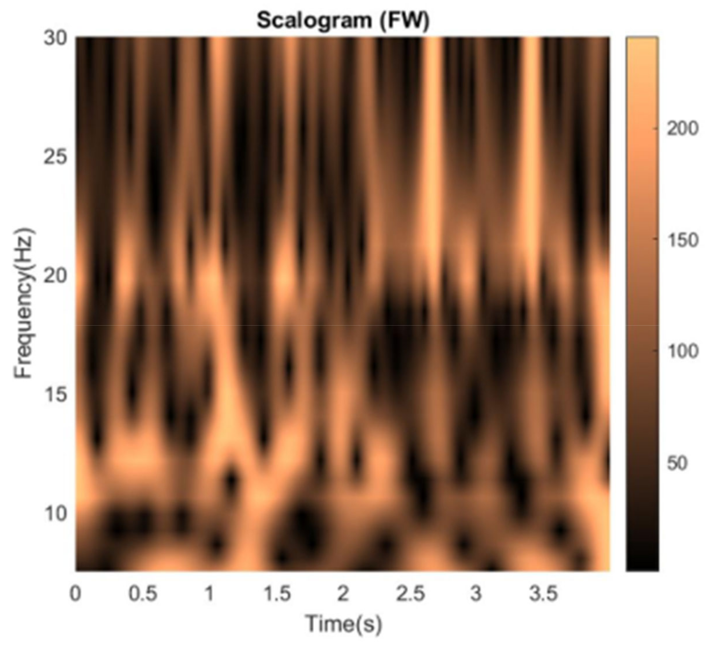
The continuous wavelet transform (CWT) converts a signal from the time domain into the time-frequency domain. Unlike the Fourier Transform, which lacks time localization and performs poorly with non-stationary signals like EEG, the CWT addresses these limitations by producing wavelet coefficients. These coefficients can be used to determine the amplitude or power of the signal's frequencies. Mathematically, the CWT involves convolving the signal of interest (in this case, the EEG signal) with a wavelet kernel over several frequencies [34]. In this project, the analytic Morse wavelet is used, with a symmetry parameter (gamma) equal to 3 and a time-bandwidth product of 60. This wavelet was chosen because it has been shown to produce excellent results with the current EEG dataset, as demonstrated in [17]. The CWT generates time-frequency plots known as scalograms (Figure 10), which can be utilized with convolutional neural networks (CNNs) like GoogLeNet for further analysis.
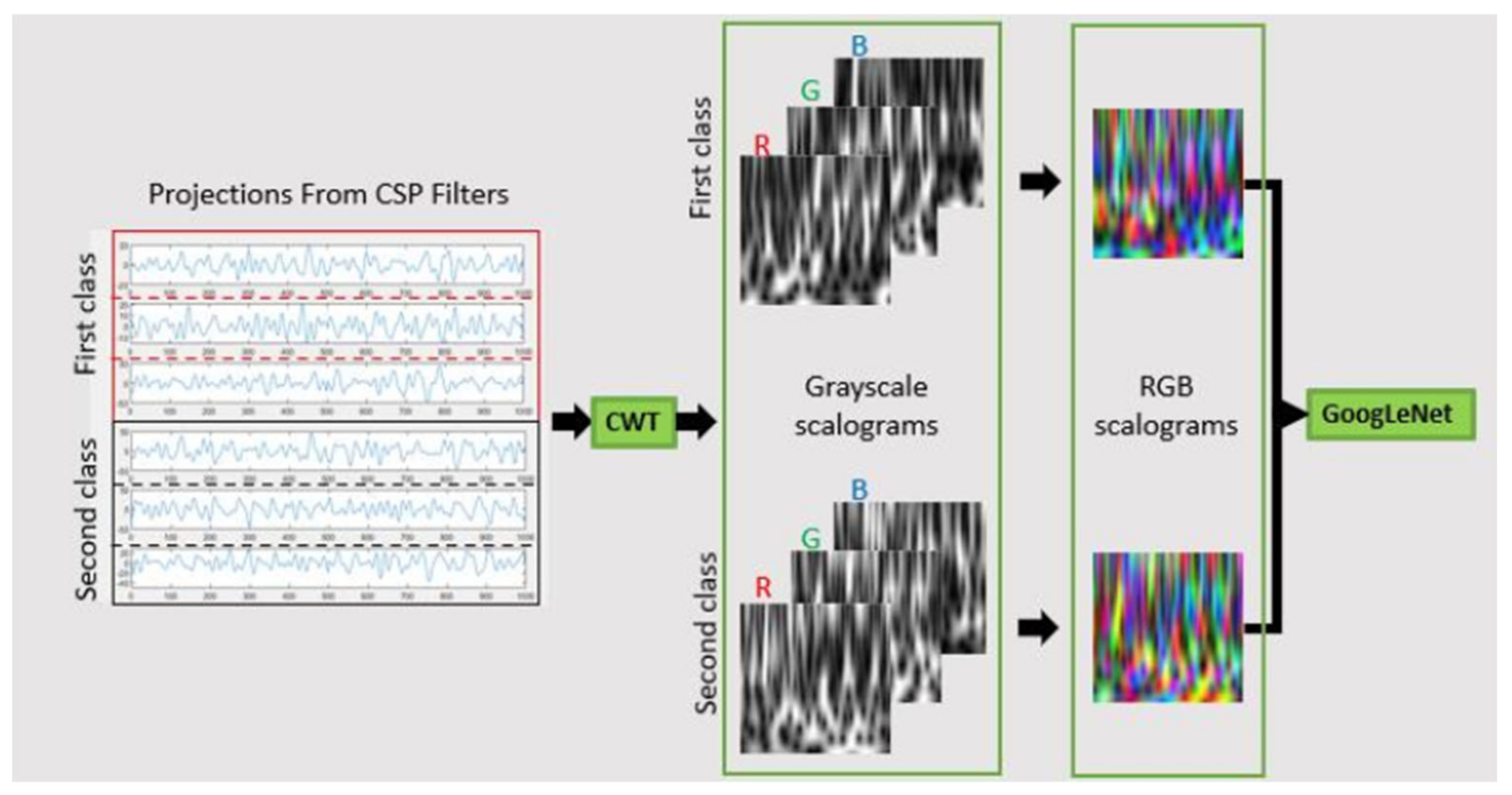
The time projections obtained from CSP filters are transformed by CWT to generate grayscale scalograms. The 3 scalograms corresponding to the first and the second class are taken as individual RGB channels, which are flattened to form two RGB scalograms, one for each class. These are passed into GoogLeNet for classification between the first and the second class. The RGB conversion is necessary since GoogLeNet only accepts images with 3 color channels, and the information from 3 projections can be gathered into one object. The CSP-CWT procedure can be seen in Figure 11.
Transfer learning is used with this pretrained network to reduce the computation cost and time. Only the last two layers (fully connected layer and softmax layer) are modified during the transfer learning. 80:20 ratio is used for splitting the training set and test set from the scalogram image set. Images are resized to 244 x 244 x 3 since this is the required dimension of the input images when using GoogLeNet. During training, the weights of the first 10 layers are frozen. Mini-batch size of 5 is used with 10-30 epochs to train each class. The learning rate is set to 0.0003.
Figure 12. Layers of GoogLeNet as displayed by the MATLAB network analyzer. The last 3 layers (shown in red) are the replaced layers for transfer learning. The model under analysis is ML-CSP-OVR, whose softmax layer is showing 4 output nodes since the model is a 4-way classification model.
Preprints 115483 g012
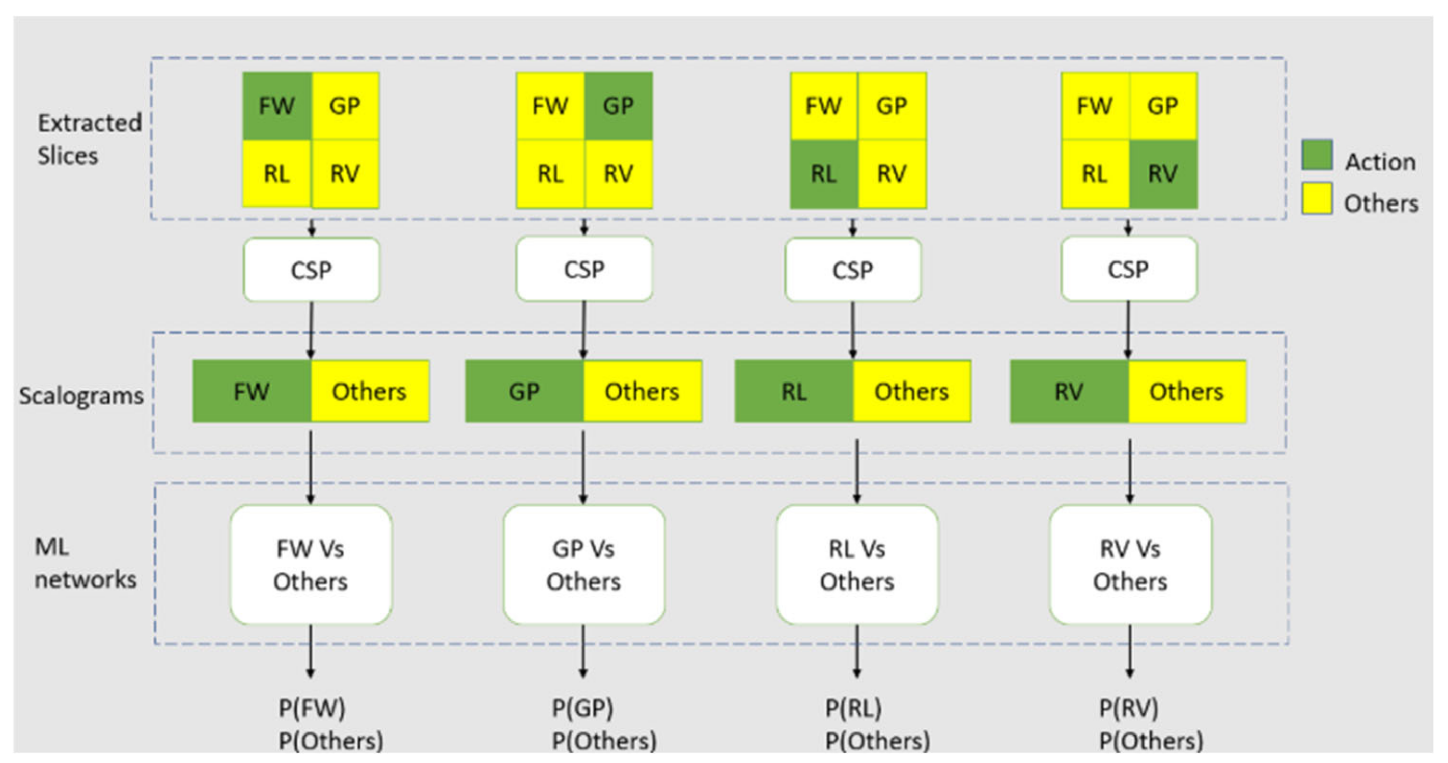
This model is based on the baseline model but extended in the classification step to transform the baseline model into 4-way classifier. However, since CSP is restricted to 4.5. ML Model 1 binary pairs/classification, the conventional way of using SoftMax layer to do 4-way classification does not work. This results in the complicated procedure of using comparators to do the 4-way classification (See Figure 9 for the pipeline).
The model is shown in Figure 13, where the inputs are taken from the pre-processed slice data in the form of 'One Vs Others', with one pitted against a group of the other actions for training. The amount of data for one action is set to be the same with the amount of data for the other group. The model is also be tested with the case where the amount of data is not the same. 4 pairs of such groups (FWvsOthers, GPvsOthers, RLvsOthers, RVvsOthers) are collected for the training set and passed into the 4 ML networks, one for each pair. In the classification step, a group of datasets collected from FW, GP, RL, and RV are used to create the test set for the model (See Figure 14 in the next section). The classification step is the same as the one in ML Model 2.

4.7. ML Model 2

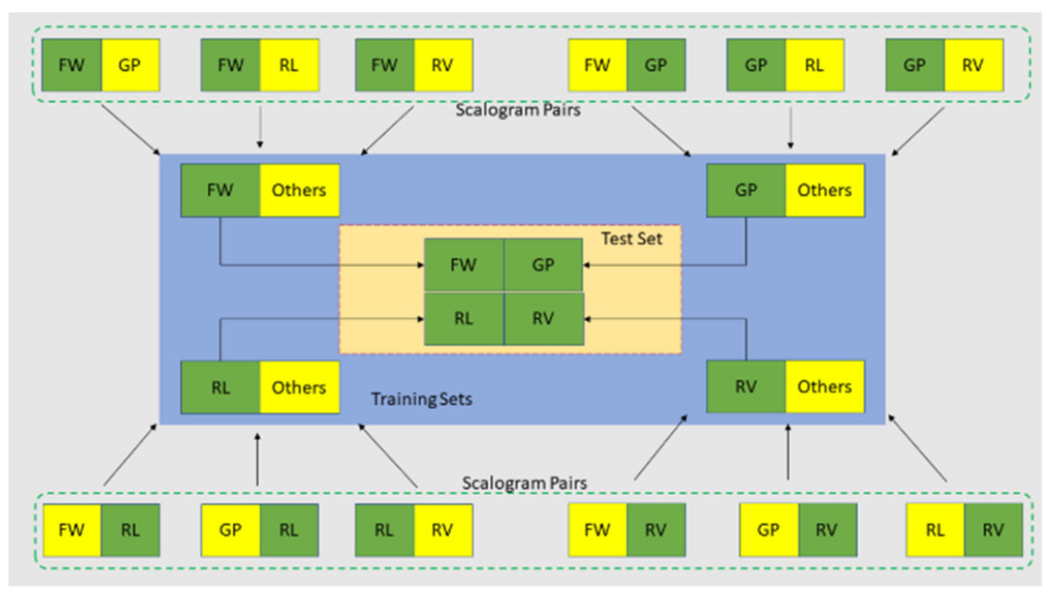
Model 2 is almost similar to Model 1, with the key difference being the source of the training inputs. Instead of using pre-processed slices, the inputs for Model 2 are derived from scalogram pairs after their generation. For example, for the FW vs. Others pair, 'FW' data is collected from FW_GP, FW_RL, and FW_RV, while 'Others' data is compiled from the GP, RL, and RV segments of the three mentioned pairs. The test set, consisting of four classes (FW, GP, RL, and RV), is assembled from the input training data. Specifically, the FW class in the test set is taken from the FW segment of the FW/Others set, and the same approach is applied to the other three classes (as illustrated in Figure 13).
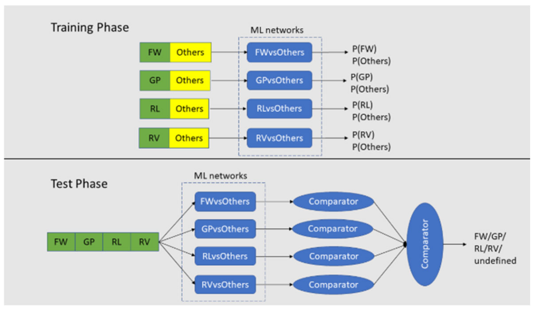
Figure 15 shows the overall framework of how the training sets and the test set are used in the training stage and the test stage of the model.
With these FW vs Others, GP vs Others, RL vs Others, and RV vs Others data, the model is trained and validated using 80:20 training and validation data split. The data in Figure 16 shows the validation accuracy for 4 pairs of networks (1. FW vs Others, 2. GP vs Others, 3. RL vs Others, and 4. RV vs Others). The validation is done on the respective 20% validation set.
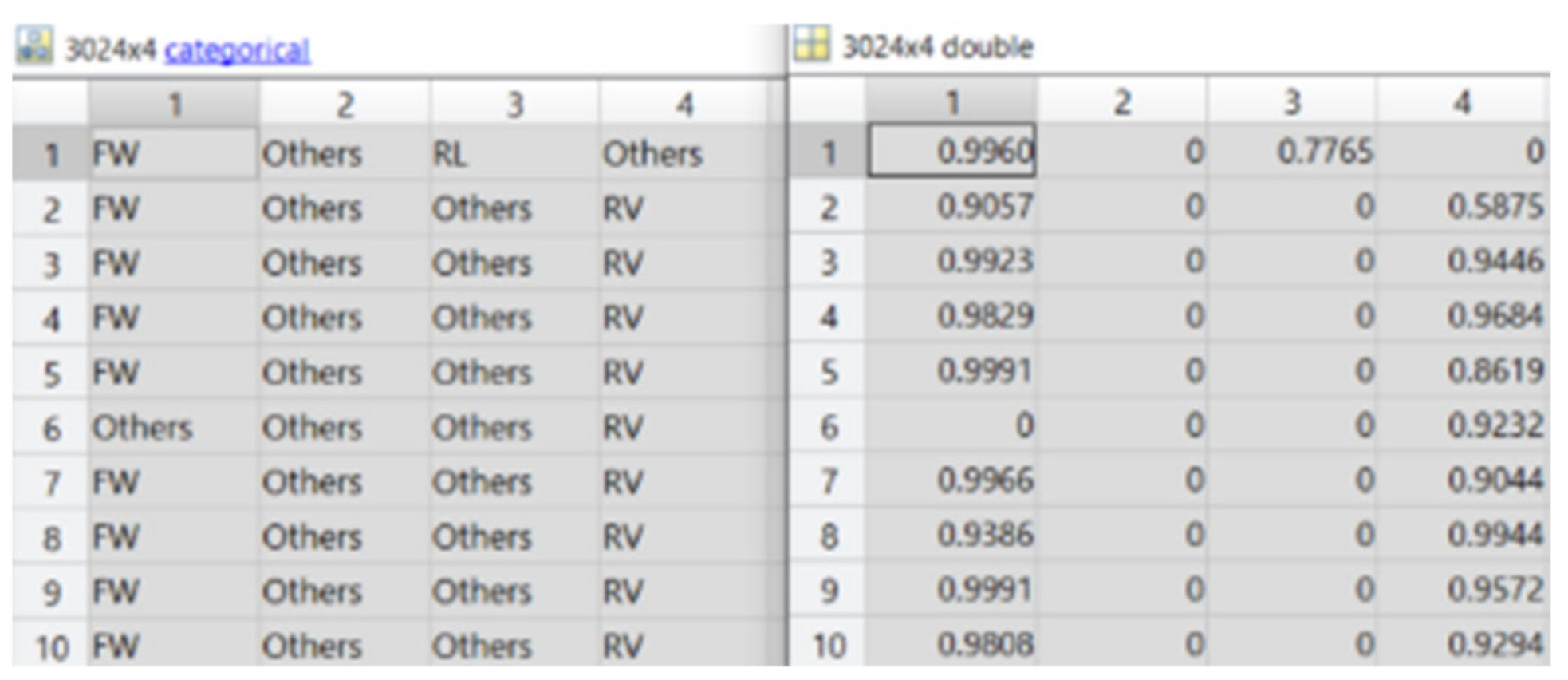
Figure 17 shows the predicted labels from the 4 networks and their corresponding probabilities. It is to be noted that the probabilities for 'Others' are set to 0 since 'Others' class does not have much meaning in this project.
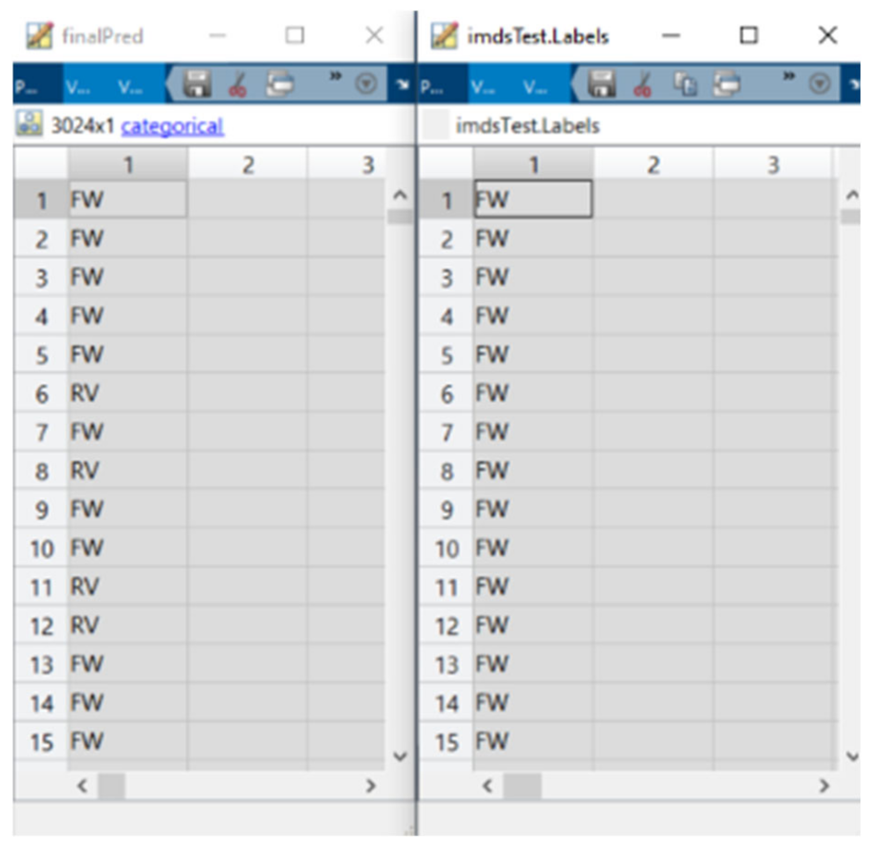
Once that procedure has been done, out of the remaining probabilities, the highest one is picked and its corresponding event. The final predicted classes are then compared with the true labels to calculate the accuracy of the model. In Figure 18, the left one shows the final predictions whereas the right one shows the true labels of the test set.

4.8. Model 3(Conceptualized)

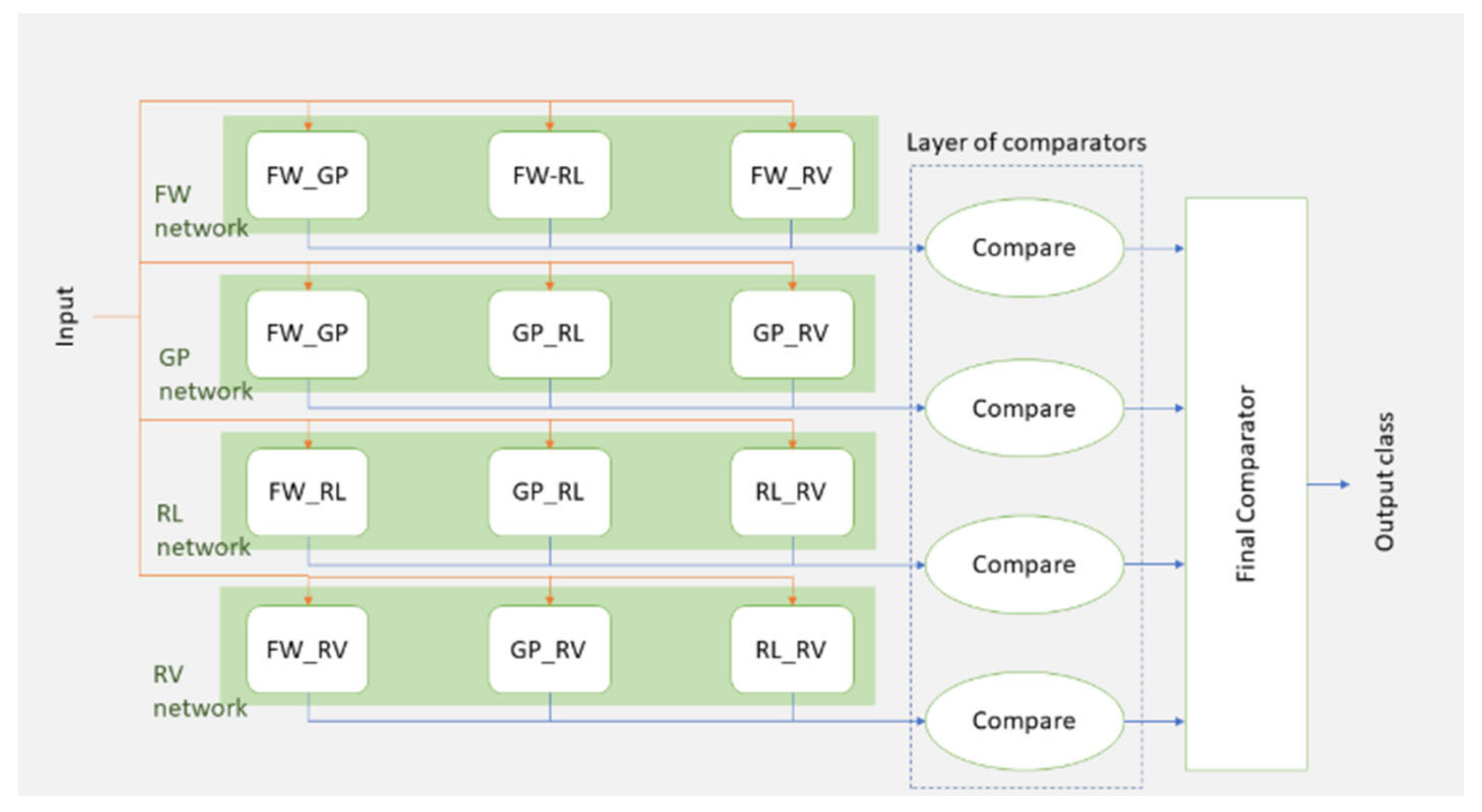
The last model (Figure 19) employs a technique described in the original CSP paper: majority voting of all pairwise classifications. For instance, an action is classified as 'FW' only if FW-GP, FW-RL, and FW-RV all return FW; otherwise, it is deemed indecisive. This method is used more leniently, where if at least two of the three pairs produce the same classification result, that result is accepted. This selection process occurs within a layer of comparators. If each network group outputs a different class, the comparator yields 'undefined'. The four outputs from the comparator layer are fed into a final comparator to select the class with the highest probability. In this ensemble of CNN networks, six networks are trained and interconnected in a complex manner to determine the final class via majority voting. However, it should be noted that this model was not implemented because Models 1 and 2 did not perform well on the 4-way classification task.

4.9. ML-CSP-OVR

Using CSP OVR instead of the vanilla CSP allows the model to do the multiclass classification without being restricted to binary classification pairs. CSP One Vs Rest (OVR) has been implemented using the combination of algorithm from [9] and [12]. This method is selected as the best method due to its low computational cost and simple classification procedure without the medium SoftMax steps due to the binary classification pairs. Figure 20 illustrates the pipeline of the ML-CSP-OVR model.
Firstly, slices of FW, GP, RL, and RV are processed using the CSP-OVR algorithm to calculate the spatial filters that best differentiate the four classes. After obtaining the spatial filters for each class, the first three filter components from each filter matrix are selected, as these are the most effective at distinguishing the classes. Like the baseline system, these selected filters are applied to the four event signals to create projection signals used for class discrimination. Continuous Wavelet Transform (CWT) is then performed to generate scalograms, which are subsequently fed into GoogLeNet for the 4-way classification.

4.10. Performance metrics

To measure the performance of the models, 5 types of evaluation are used: (i) accuracy, (ii) precision, (iii) sensitivity, (iv) specificity and (v) F1-score. The mathematical equations of these are as follows:
Accuracy = TP TP   +   TN   + FP + FN  
Precision = TP TP   +   FP
Sensitivity = TP TP + FN
Specificity = TN   TN   + FP
F 1   Score   = 2 × Precision   ×   Sensitivity Precision   +   Sensitivity
where TP = True Positive, TN = True Negative, FP = False Positive, and FN = False Negative [45].
Feature extraction in EEG signal processing involves identifying and isolating relevant information from raw EEG signals to enhance classification or analysis. This process typically starts with preprocessing steps like bandpass filtering and artifact removal to ensure clean data. Time-domain features such as amplitude, power, and zero-crossing rate provide insights into the signal's intensity and variation. Frequency-domain features like power spectral density (PSD) and band power offer a breakdown of the signal's energy across different frequency bands, which is crucial for understanding various cognitive states. Time-frequency domain features, including Wavelet Transform (WT) and Short-Time Fourier Transform (STFT), capture how the signal's spectral content evolves over time, which is particularly useful for non-stationary EEG signals. Spatial features like Common Spatial Patterns (CSP) and Independent Component Analysis (ICA) enhance the differentiation between brain states by focusing on spatial patterns of brain activity. Non-linear features such as fractal dimension and Lyapunov exponent provide additional insights into the complexity and chaotic nature of EEG signals. Often, a combination of these features is employed to capture the full range of information in the EEG data. After feature extraction, feature selection techniques like Principal Component Analysis (PCA) are applied to reduce dimensionality before feeding the features into classification models, which can range from simple linear classifiers to advanced machine learning algorithms like Support Vector Machines (SVMs) or deep neural networks. This systematic approach to feature extraction is critical for developing accurate and reliable EEG-based applications, including Brain-Computer Interfaces (BCIs).
To summarize, the data processing and feature extraction steps in the study began with data collection from 12 participants, each performing 10 sessions of grasp and lift (GAL) trials. Trials exceeding 28 were discarded to standardize the dataset, and visual inspection ensured a consistent 3-second duration for each trial, leading to the exclusion of participant 7 due to inconsistencies. The raw EEG signals were filtered to remove noise, and four 1-second segments were extracted from the filtered data, each 500 samples long. Common Spatial Patterns (CSP) were employed to extract spatial features, selecting six spatial filters to distinguish between conditions. Event-Related Desynchronization/Synchronization (ERD/ERS) features captured power changes in specific EEG frequency bands associated with motor activities. CSP filters produced time projections for classification, with steps including covariance matrix estimation and whitening transformation. The initial model used K-Nearest Neighbors (KNN) with 3 nearest neighbors and 10-fold cross-validation, achieving accuracies of 57.23% for forward-reverse pairs and 50.87% for grasp-release pairs. Convolutional Neural Networks (CNNs) were later used for final classification, validated with an 80:20 training-validation split, although Model 3, which involved majority voting, was not implemented due to performance issues. Evaluation metrics such as accuracy, precision, sensitivity, specificity, and F1-Score were calculated using True Positive (TP), True Negative (TN), False Positive (FP), and False Negative (FN) values. This detailed description, including parameters and specific implementations, ensures that readers can reproduce the experimental results accurately. Furthermore, feature extraction for both classes can be performed simultaneously by first applying preprocessing steps to the entire dataset, then extracting features from the entire set before splitting it into different classes. This approach involves applying techniques like PCA or ICA to the full dataset, selecting the most relevant features, and then dividing the data into classes or training/testing sets. This ensures that the features are representative of the entire dataset, leading to more robust and generalizable models.

5. Measurement Results

For the KNN classification in the preliminary study, only intersubject classification is used, incorporating data from all participants. It is important to note that in this paper, for the baseline system as well as Models 1 and 2, the intersubject classification is conducted without using leave-one-out testing. This means that a separate test set from one participant, which is left out of both training and validation, is not used. However, given the satisfactory performance of the ML-CSP-OVR model, the test paradigm is extended to include leave-one-out intersubject classification. For the GoogLeNet classification, both intrasubject and intersubject classifications are utilized. In the baseline system, intrasubject classification is performed for all participants. In the three variant models, intrasubject classification is conducted for three participants: P1, P5, and P12. Intersubject classification uses data from participants 1 to 11, excluding participant 7 as previously mentioned.

5.1. Preliminary Study Model

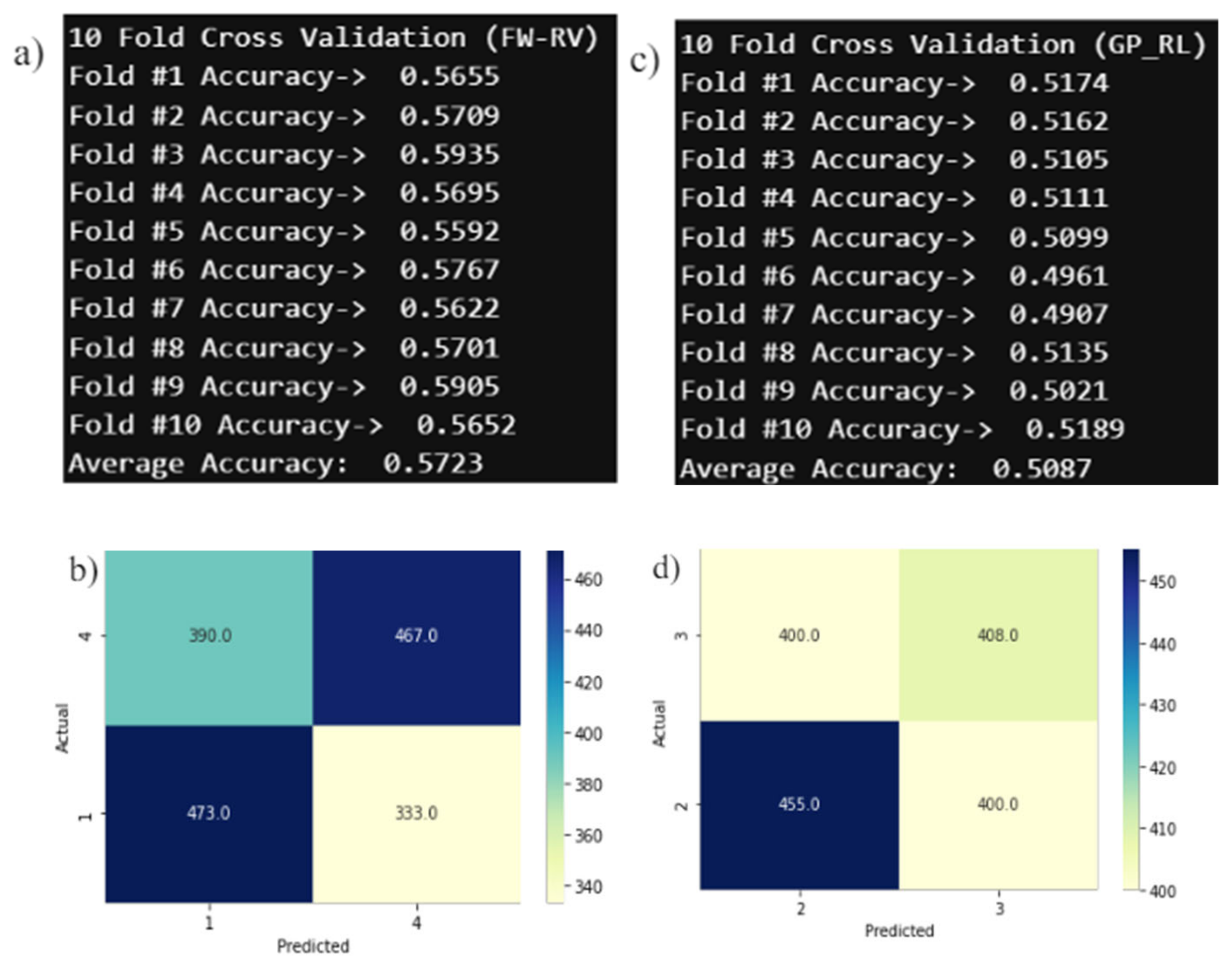
The model uses K Nearest Neighbor classification which can only achieve the average accuracy of 57.23% for forward-reverse pair, and the average accuracy of 50.87% for grasp-release pair, using the time and frequency features as shown in Table 3, Section 4.4. The classification is done with the 3 nearest neighbors as mentioned before and with 10-fold cross validation scheme. Either increasing or decreasing the number of neighbors results in significant drop in accuracy.
Figure 21 shows that the performance of the classifier on the dataset is below 60%, which is expected due to the nature of the dataset (Figure 14, Section 4.4.2). The result could be improved if the features are extracted from the spatially and temporally filtered signals rather than using only the temporally filtered signal. However, these results are left unimproved since the objective of the preliminary study is to gain the overall picture on what is involved in neural signal processing and classification.

5.2. Baseline Model

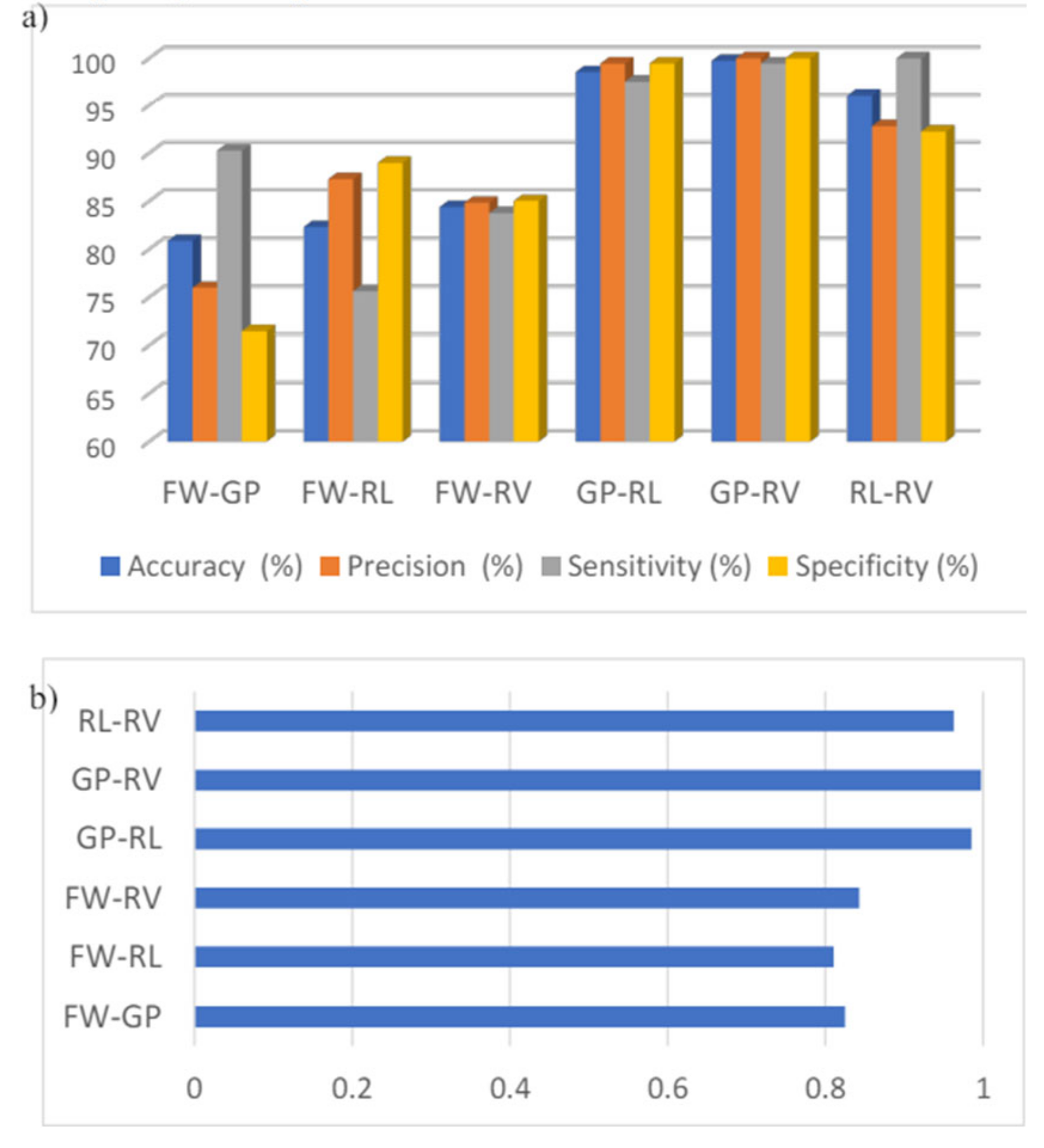
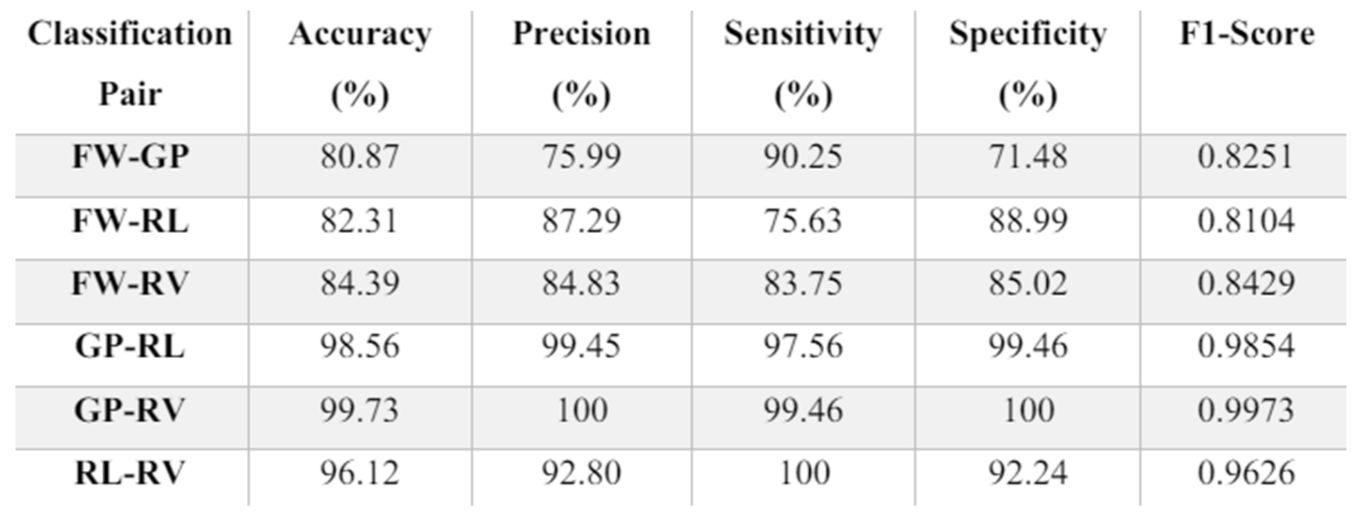
With a total number of 2772 of trials (11 participants x 9 series x 28 trials) and with 3 color channels (RGB), the number of grayscale scalograms produced per event is 8316. Since one classification involves a pair of two events, the total number of images is 16632. After flattening the separate grayscale scalograms, the total number of RGB images per pair of classification is 5544. This feature extraction process can take up to 3-4 hours for a single classification. 5544 scalograms are split into training and validation set 80:20 ratio as mentioned before in Section 4.5.1. Using Equation. (16)-(20), the five evaluation scores for the classifications are obtained. Intersubject classification is conducted between 2 unique pairs of events, resulting in 6 pairs for classification across all 11 participants. Table 4 indicates that the baseline system (average values) achieves a range of accuracy from 80.87% to 99.73%, with nearly perfect accuracy. Precision, sensitivity, and specificity range from approximately 71% to 100%, with the lower end of the range predominantly observed in the first three pairs. The average accuracy, precision, sensitivity, and specificity across all 6 pairs are 90.33%, 90.06%, 91.11%, and 89.53%, respectively. The average F1 score is 0.90. From Figure 22-a, it is evident that the performance metrics for the first three groups are about 10-30% lower than those for the last three groups. The F1 score follows a similar trend between these two sets of groups (Figure 22-b). This performance drop in the first three groups could be attributed to the forward hand movement (FW) event, as these groups all involve the FW event. Enhancing accuracy might be possible by adjusting the FW slices to a better temporal location. Refer to the intra-subject classification for another potential cause of this performance drop.
The training and validation progress plots of the classifier for FW-RV and GP-RL.
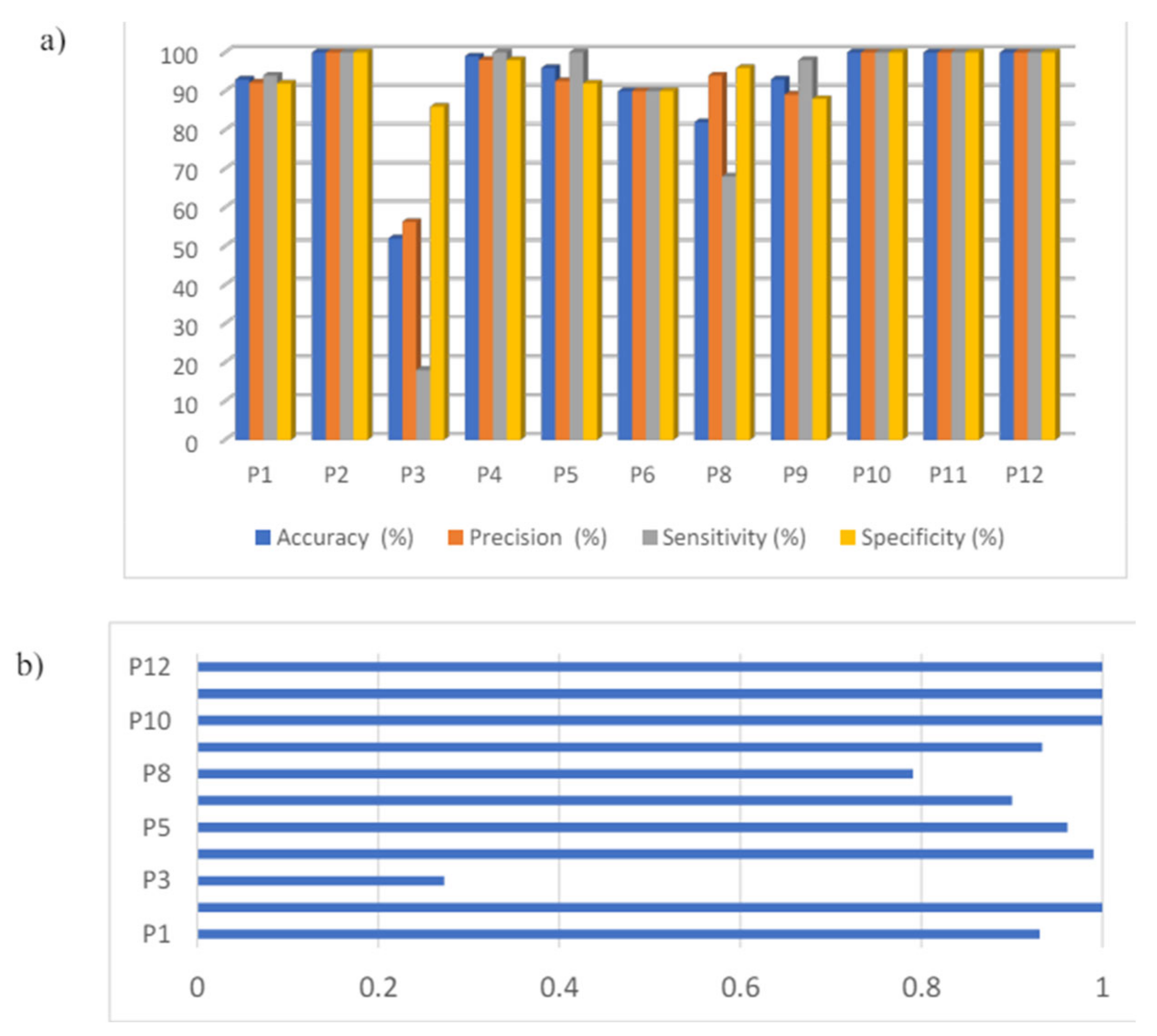
For intrasubject classification, the pair with the lowest accuracy from intersubject classification (FW-GP) is selected. The data for this pair is separated by individual participants, and classification is performed on these individual groups. As expected, both accuracy and F1 score improve for all participants in intrasubject classification, except for participant 3 (see Figure 23 (a) and (b)). The low accuracy score for intersubject classification might be due to participant 3's forward hand movement data, although further research is needed to confirm this. For some participants, the baseline method achieves perfect scores for all performance metrics, as shown in Table 5. The average accuracy, precision, sensitivity, and specificity across all 11 participants are 91.36%, 92.01%, 88%, and 94.73%, respectively.
The training and validation progress plots of the classifier for participant 2 and participant 5.
Comparison of performance between the baseline system and that of the selected paper Since the classification of paper [17] is done on event Vs non-events, direct comparison cannot be made. However, due to certain similarities such as events of interest (e.g., GP, RL), it is still possible to use the results of the paper as a reference. The results of the paper are show in Table 6.
To compare against the results from the paper, an average is performed on the same events to get a single digit since the baseline system classification is done on pairs of individual unique events. For example, grasp related events, the performance scores GP-FW, GP-RL, GPRV are averaged for comparison. These average values are shown in Table 7
From Table 6 and Table 7, it can be observed that the performances of the two systems are very close. Of course, as mentioned before, these comparisons are made not in terms of direct measurement but in terms of measurement that can give a general idea/pattern on the performance of the two systems.

5.3. ML Model 1

Intrasubject classification
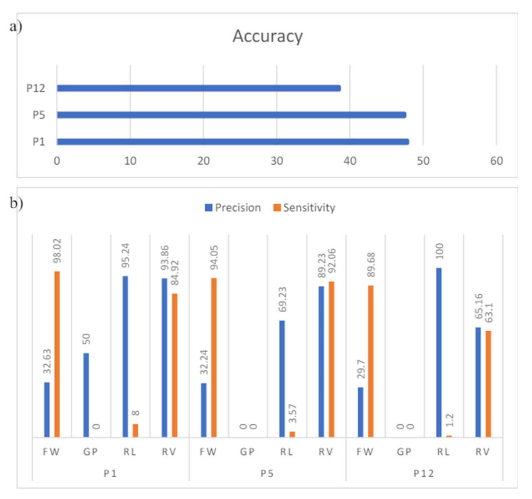
Figure 24 (a) shows that the accuracy of the system for all the selected participants falls below 50% with the lowest at 38.49%. Even though it is performing higher than random chance, which is at 25% for 4 classes, this accuracy score shows that the system is not very reliable. Figure 24 (b) also shows that for some pairs of all 3 participants, the precision and sensitivity can go as low as 0%.
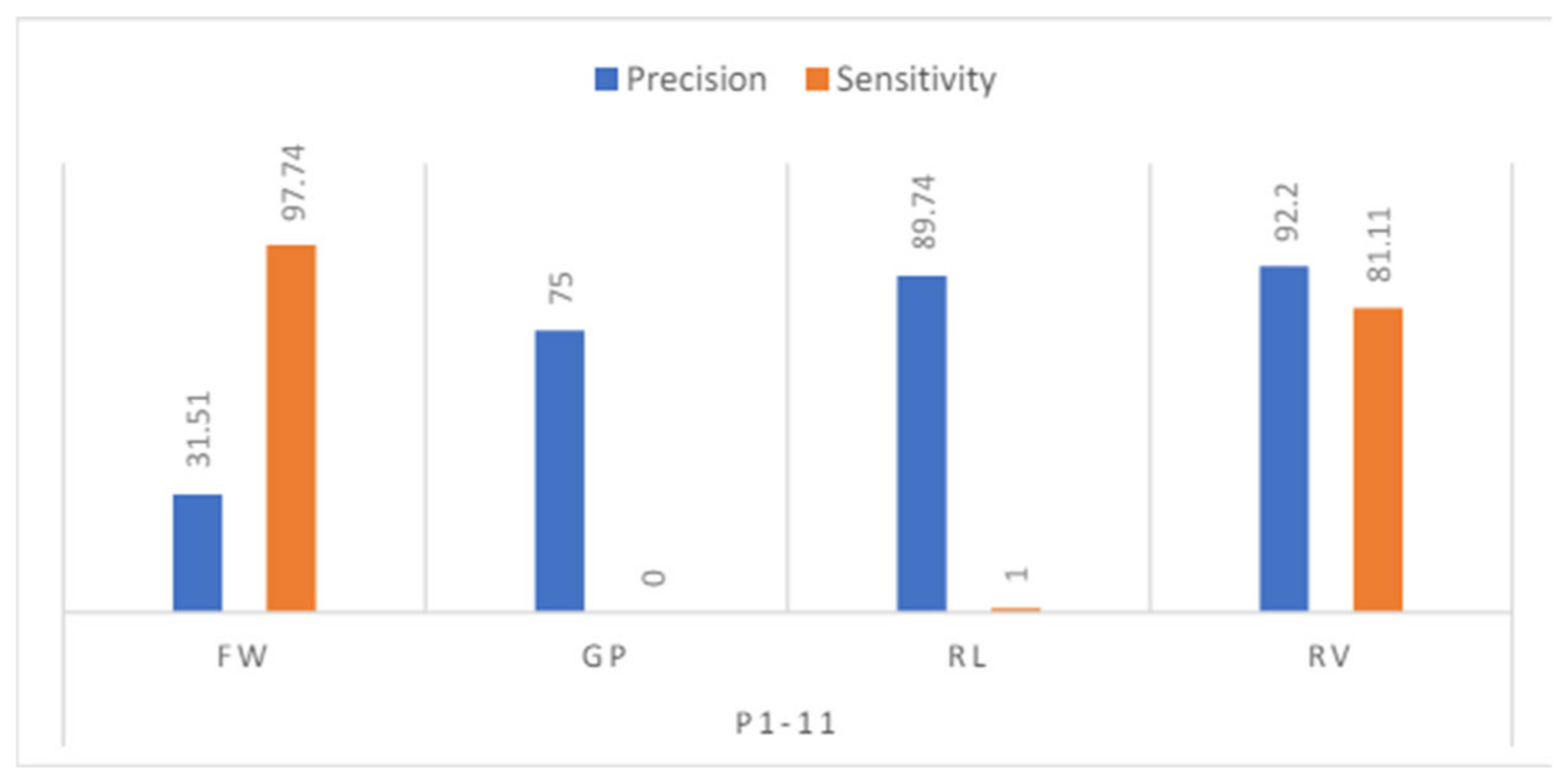
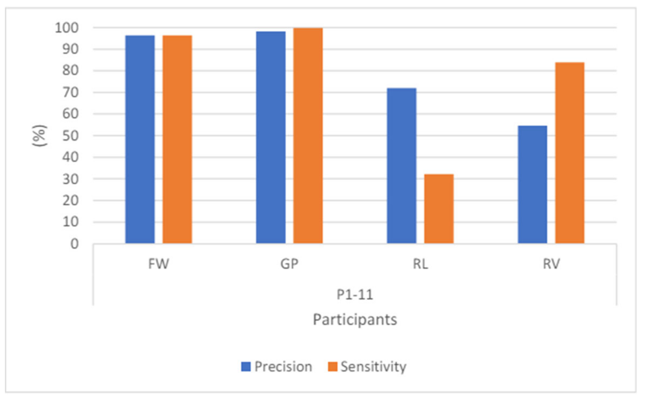
Accuracy of the intersubject classification for this model results in 45.12%. Figure 25 shows the sensitivity of GP and RL performing at 0% and 1% respectively, indicating that the model is not reliable at all for these two cases. The model performs quite well for the RV action, with both sensitivity and precision higher than 80%.
One explanation for these low scores is as follows (refer to Section 4.6, Figure 19): the idea of grouping FW as one group and other actions as another group is to allow the CSP to generate filters that create FW vs. Others scalograms. These scalograms are then used to train the 'FW vs. Others' network, with the same method applied to the other three branches. The test set is created by combining FW, GP, RL, and RV from the scalogram pairs. Focusing on one branch, 'FW vs. Others,' we can discuss the issue further since the same logic applies to the other branches. When the 'FW vs. Others' network predicts the test set labels, the assumption is that if GP, RL, or RV are tested, the network should predominantly classify them as 'Others' since they are not FW. However, because GP, RL, and RV are grouped as one pair when creating the input slices for this branch, the CSP filter turns this group of three into a single scalogram with characteristics that combine all three rather than their individual traits. In the test set, the FW, GP, RL, and RV scalograms retain the characteristics of individual actions, causing the 'FW vs. Others' network to predict the 'Others' class less frequently than the individual action classes. Since both intrasubject and intersubject classifications are not performing well, another model is explored, leading to the creation of ML Model 2. Given the theoretical explanation for the model's poor performance, ML Model 2 is designed to train the ML networks with scalograms that display individual characteristics rather than combinatorial ones.

5.4. ML Model 2

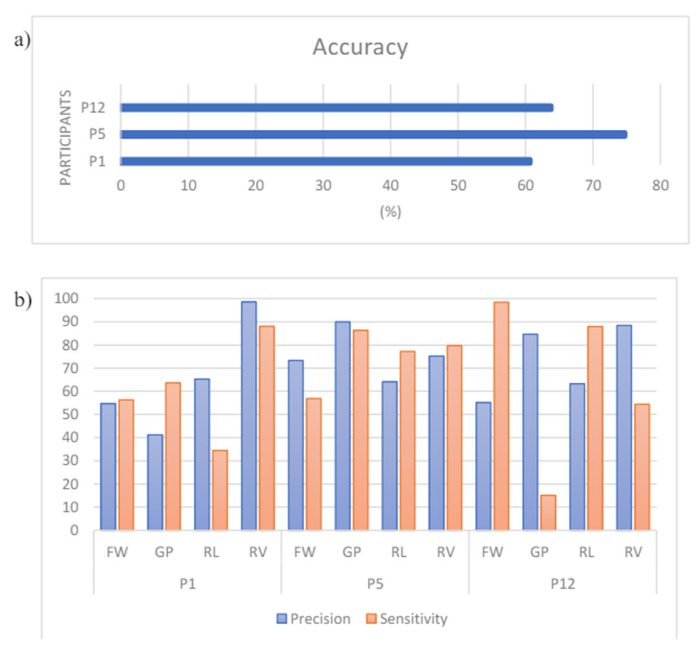
Figure 26 (a) shows that the accuracy of this model is better than that of the previous one for the same participants. Since P5 accuracy is obtained to be 74.7%, it can be inferred that for certain participants, the model accuracy can get up to about 75%. The precision and sensitivity in Figure 26 (b) also show that Model 2 performs with much reliability than Model 1.
Intersubject classification
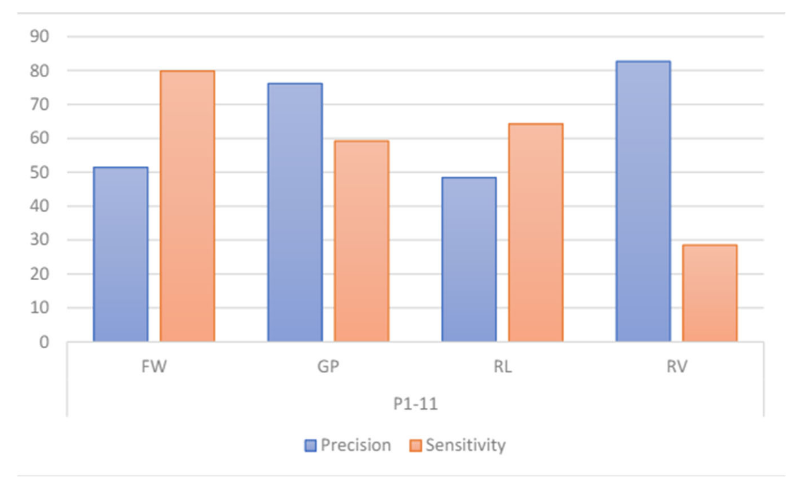
Figure 27 shows the precision and sensitivity of participants 1 to 11. Even though the sensitivity for the RV pair is quite low at 28.5%, the intersubject classification of model 2 is better than that of model 1. The accuracy achieved is 57.88%.
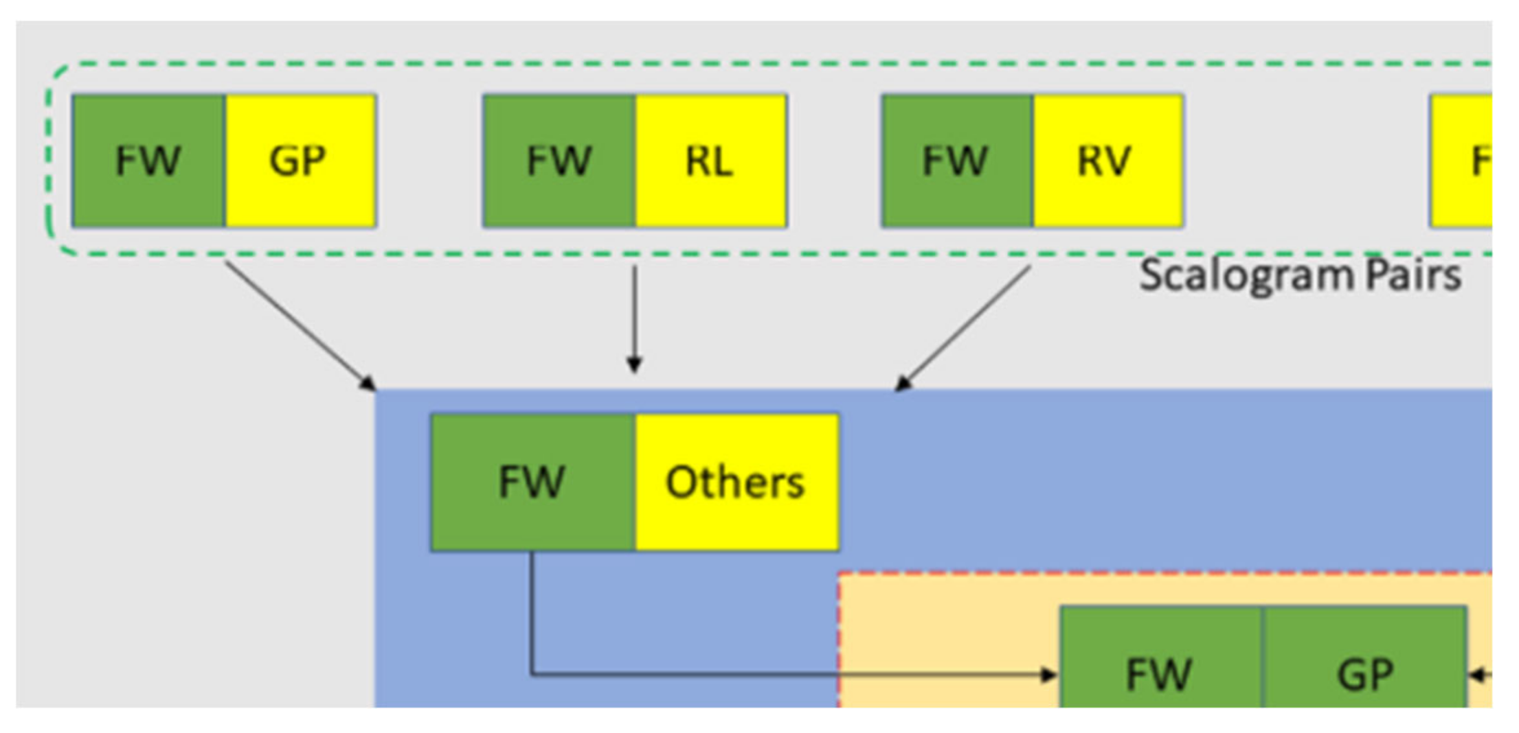
Since Model 2 has shown improved performance for both intrasubject and intersubject classification compared to Model 1, it suggests that the explanations for Model 1's low performance are valid to some extent. One possible reason for the lower scores in Model 1 could be the binary classification approach used in the CSP method. Figure 28 presents a segment of the framework depicted in Figure 20, Section 4.7, for easier reference. The three scalogram pairs—FW_GP, FW_RL, and FW_RV—are all distinct because CSP ensures that only a pair of two classes is distinguishable from each other. In the FW_GP pair, CSP maximizes the distinguishability between FW and GP, and is similar for the other pairs. This results in the two FW groups from FW_GP and FW_RL being different, as CSP ensures that FW is distinct from GP in the first pair and distinct from RL in the second pair.
The distinctions made by CSP in binary classification can lead to issues. For instance, FW from the FW_GP pair might exhibit similar characteristics to RL from the FW_RL pair. This problem can extend to all scalogram pairs used for creating the training and test sets. Since this issue arises from the binary classification nature of CSP, it is necessary to adopt a method capable of multiclass classification. Consequently, a third model is implemented using the CSP-OVR method, which is designed for multiclass classification.

5.5. ML-CSP-OVR

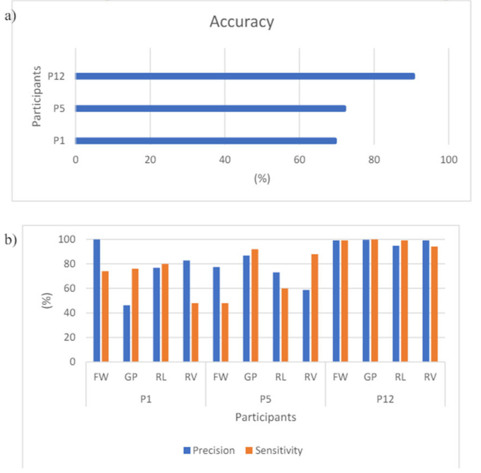
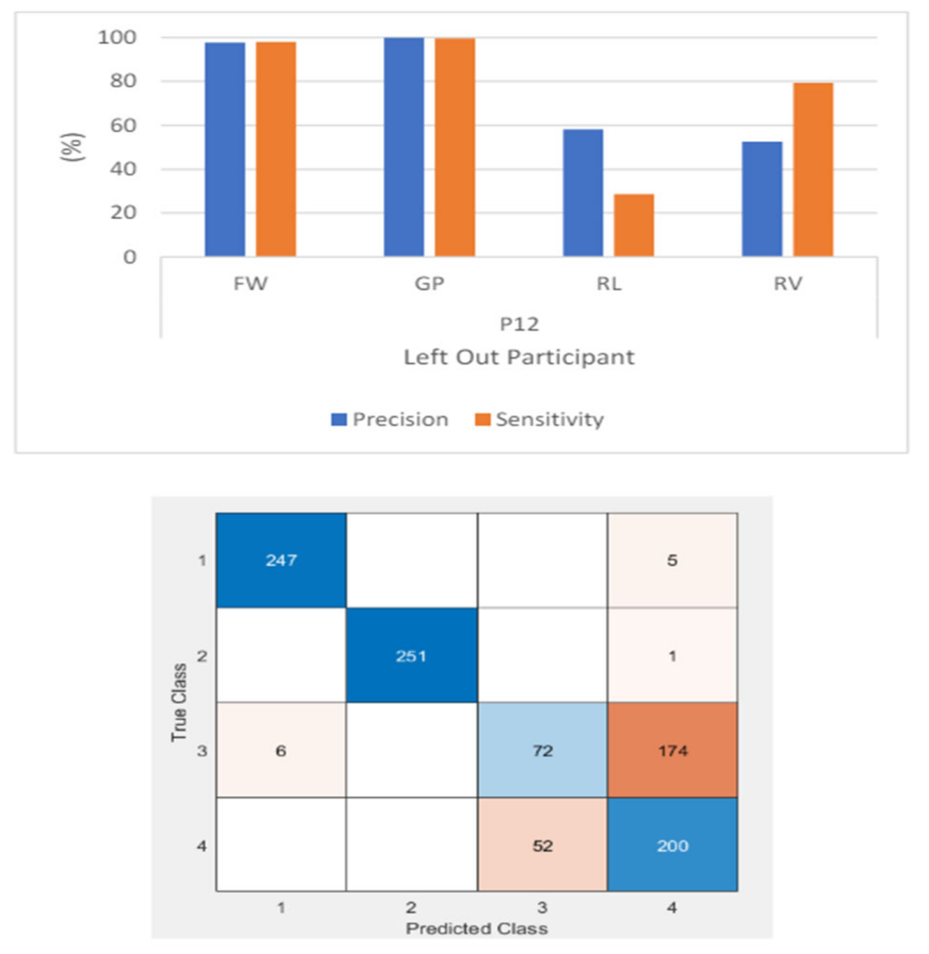
Among the three ML models, ML_CSP_OVR performs the best for both intrasubject and intersubject classification. For intrasubject classification, as shown in Figure 29, participant 12 achieves an accuracy of 90.5%, with both sensitivity and precision exceeding 90%. The lowest accuracy is 69.5% for participant 1. For intersubject classification, the accuracy achieved is 78.08%, with precision and sensitivity exceeding 88% for 2 out of 4 classes (see Figure 30).
Intersubject classification
Intersubject classification (Leave One Out)
Given the strong performance in both intrasubject and intersubject classifications, the task is extended to include intersubject classification with leave-one-out. This is the most challenging task, as EEG signals are known to be subject-specific, differing from one participant to another. In this setup, participant 12 (P12) is excluded from the training set, meaning the machine learning model has not seen any data related to P12 during training. After training, P12 is used as the test set. As shown in Figure 31, the ML-CSP-OVR model performs similarly to the intersubject classification without leave-one-out, achieving an accuracy of 76.39%. However, the confusion matrix indicates that the model struggles to discriminate between the RL and RV classes. This difficulty may be due to the proximity of the two actions, which are executed almost simultaneously. The extracted slices for the RL and RV classes overlap, leading to similarities that make it challenging for the model to differentiate between the two classes.
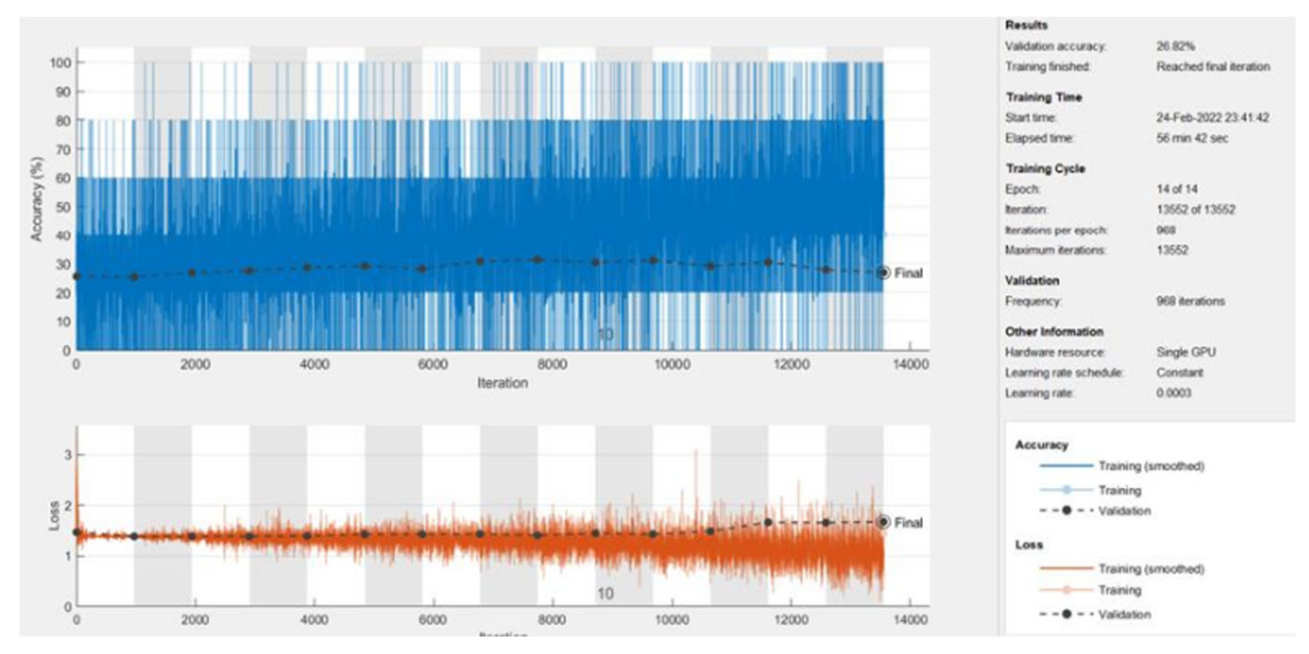
Classification with GoogLeNet classifier without using the CSP-OVR was conducted to compare the performance of the CSP-OVR method. The training and validation set is made of scalograms, generated using only the continuous wavelet transform. Figure 32 shows the result of this classification, whose accuracy is 26.82% which is very close to 25% (the probability of randomly guessing 4 classes).

5.6. Overall comparisons across the three 4-way classifiers

Intrasubject classification
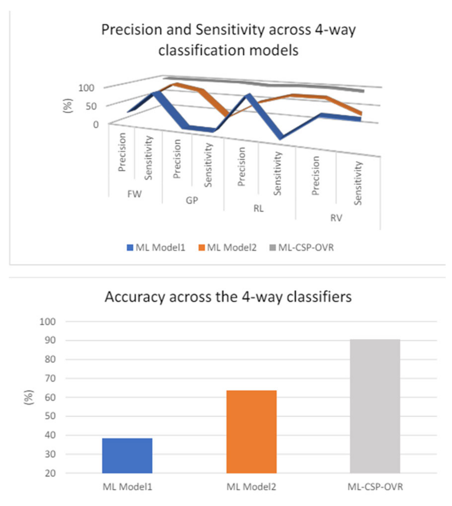
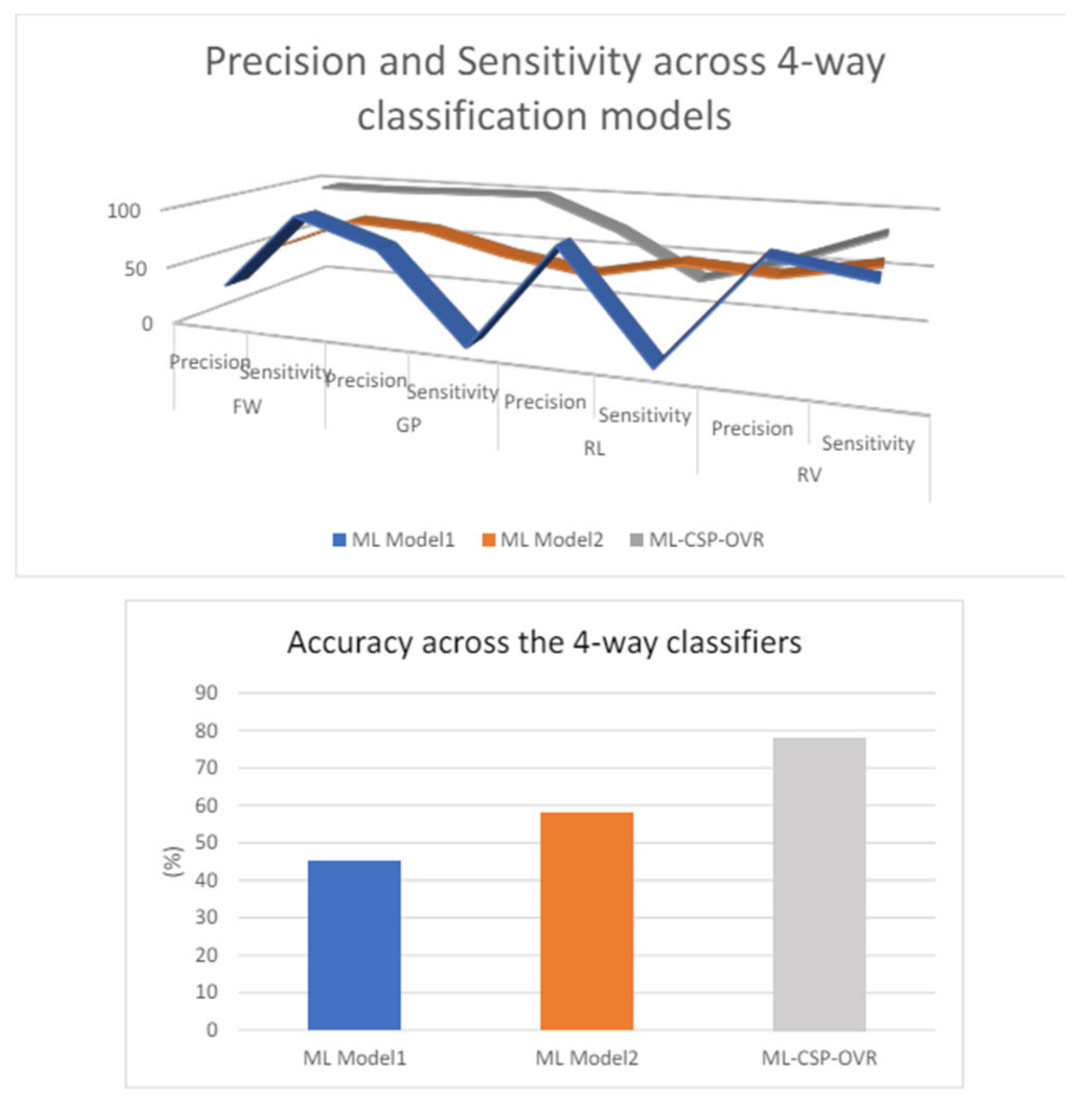
Figure 33 confirms further that ML_CSP_OVR performs better than the other 2 models, in terms of precision, sensitivity and accuracy. The measurement data is obtained on participant 12.
Figure 34 also shows that ML-CSP-OVR performs better than the other multiclass classifier models. Even though there is a dip in the sensitivity and precision for RL and RV, the overall trend of the ML-CSP-OVR still performs better than the other two. For the accuracy, ML-CSPOVR manages to achieve approximately 20-40% better result than the other two models.

6. Discussion

Analysing the factors affecting the performance of EEG signal processing and classification systems involves considering multiple aspects of system design, data quality, and method implementation. One crucial factor is dataset quality and size. A larger and cleaner dataset often leads to better model performance. Small or noisy datasets can result in overfitting or poor generalization. To improve, we could increase the dataset size through data augmentation techniques or collect additional data. Enhancing data quality by applying robust preprocessing methods to reduce noise and artifacts also contributes significantly to better performance.
Feature extraction techniques play a pivotal role in determining system performance. Different methods, such as wavelet transforms, ICA, or PCA, affect the relevance and quality of the features used for classification. Experimenting with various feature extraction techniques, including hybrid approaches, can help identify the most effective ones for our specific dataset. Additionally, exploring deep learning-based feature extraction methods may offer significant improvements if computational resources permit. The choice of classification algorithms is another critical factor. Algorithms like SVM, neural networks, or decision trees have varying effectiveness depending on the data and features. Testing a range of classification algorithms and fine-tuning their parameters can lead to better results for our proposed work which we will implement for our future work. Utilizing ensemble methods to combine predictions from multiple classifiers can further enhance accuracy and robustness. Preprocessing and denoising techniques are essential for ensuring high-quality input data. Advanced preprocessing methods, such as adaptive filtering and artifact removal, can significantly improve the signal quality. Implementing these techniques helps in enhancing the effectiveness of the classification system.
Model complexity can also impact performance. Overfitting is a common issue with complex models, especially if the dataset is small or not diverse enough. To address overfitting, we could explore using cross-validation, regularization, and dropout techniques for our future work. Simplifying models may also help in achieving better generalization.
This proposed work classification accuracy reveals several factors influencing performance compared to recent research using similar datasets and methods. Differences in accuracy can be attributed to various elements, including dataset characteristics, feature extraction methods, model architectures, and training strategies. For instance, dataset size, quality, and diversity play a crucial role in performance. Smaller or less diverse datasets may lead to overfitting or inadequate model generalization. The choice of feature extraction techniques, such as wavelet transforms or ICA, can also impact accuracy, with some methods better capturing relevant patterns in the data than others. Model architecture and algorithm choices significantly affect performance. Variations between models like SVM, CNN, and RNN can lead to different accuracy outcomes, as each model type has its strengths and limitations depending on the data and task. Additionally, training procedures, including hyperparameter tuning and cross-validation strategies, can contribute to performance discrepancies. Effective training practices and robust validation approaches are essential for optimizing model accuracy. Several factors affect performance, including data quality and preprocessing. Issues such as noise, artifacts, and incorrect labelling can degrade accuracy, highlighting the importance of careful data handling and preprocessing. Model complexity also plays a role; while more complex models may capture intricate patterns, they can also be prone to overfitting if not properly managed. Computational resources impact model training and evaluation, as limitations may restrict the use of advanced models or extensive datasets.
This study [61] explores the use of deep learning models for classifying EEG signals from brain-computer interface applications. The authors use a dataset similar to the one that we are using and apply convolutional neural networks (CNNs) for feature extraction and classification. The deep learning approach demonstrates high classification accuracy and robustness in noisy environments. This study [62] could provide valuable insights into using advanced neural networks for EEG classification and help benchmark performance. This paper focuses on using wavelet transform for feature extraction from EEG signals, followed by classification using support vector machines (SVM). The dataset used is comparable to our standard EEG datasets. The combination of wavelet transform with SVM shows effective results in distinguishing different mental states. This study highlights the utility of classical feature extraction methods in EEG signal processing. On the other hand, this research [63] compares Independent Component Analysis (ICA) and Principal Component Analysis (PCA) for denoising and classifying EEG signals. The study uses similar preprocessing and feature extraction techniques. The comparison provides insights into the effectiveness of ICA versus PCA in different scenarios. This paper could be useful for understanding the trade-offs between these techniques in EEG signal processing. All the 3 studies above use EEG signal datasets, like our proposed work. They explore a range of methods including deep learning, wavelet transforms, and ICA/PCA, which are relevant to our feature extraction and classification approaches. Each study offers different perspectives and methods that could complement our research, from advanced neural networks to classical signal processing techniques.

7. Conclusions and Future Work

In this project, a preliminary study was conducted using time and frequency features with the KNN classifier. By using features extracted from bandpass-filtered segments of data, the KNN classifier achieved a prediction accuracy of 57.23% for the FW-RV pair and 50.87% for the GP-RL pair. A potential solution to improve this low accuracy was suggested: using CSP-filtered features as input for the classifier. However, the results did not improve, as the primary aim of the preliminary study was to understand the overall process of neural signal processing and classification. A baseline system was then developed using the CSP-CWT approach with GoogLeNet as the classifier. For intrasubject classification of the FW-GP pair, out of 11 participants, 9 achieved an accuracy of 90-100%, one achieved 82%, and another achieved 52%. For intersubject classification across six unique pairs (FW-GP, FW-RL, FW-RV, GP-RL, GP-RV, RV-RL), the accuracy ranged from 80.87% to 99.73%, with F1 scores ranging from 0.8104 to 0.9973. This baseline system demonstrated good performance in classifying the four hand movements, comparable to the system in [17]. Using the baseline system, three variants were proposed for four-way classification. Among these, the ML-CSP-OVR variant achieved the best accuracy: 78.08% for intersubject classification with combined data, and 90.5% for participant 12 in intrasubject classification. Additionally, the leave-one-out intersubject classification achieved an accuracy of 76.39%, indicating the potential of the proposed system to serve as a generalized, subject-independent solution. Future improvements to the ML-CSP-OVR system could involve integrating the FBCSP-OVR system to enhance performance, as multiple filters can improve EEG signal quality. While the GoogLeNet classifier performs well, its deep-layer structure incurs significant computational costs. To address this, a simplified CNN (SCNN) [49] could be used to reduce computational cost while maintaining good classification accuracy. Additionally, decision trees, particularly random forests, should be explored, as they have shown good performance in MI EEG analysis [19] and in the field of biomedical devices [46] and IoT technology [47,48]. Furthermore, other areas of unsupervised domain framework could be explored too [49,50]. Honestly, due to limitation in our resources, our proposed work involves twelve participants performing grasp and lift actions across a total of 3936 trials distributed over 10 series. Each participant conducted 328 trials. I agreed that the sample size or dataset should be increased to enhance the trustworthiness of our proposed work in the future.

Author Contributions

Conceptualization, Methodology, Investigation, Supervision, Resources and Software, C.L.K.; Methodology, Investigation and Data Curation, C.K.H.; Project administration, Resources, Visualization and Formal analysis, T.H.A.; Methodology, Investigation, Visualization and Formal Analysis, Y.Y.K.; Investigation, Supervision, Data Curation and Funding Acquisition, T.H.T. All authors have read and agreed to the published version of the manuscript.

Funding

This research received no external funding.

Data Availability Statement

The data presented in this study are available in this article.

Conflicts of Interest

The authors declare no conflicts of interest.

References

  1. S. Paszkiel and P. Szpulak, "Methods of acquisition, archiving and biomedical data analysis of brain functioning," in International Scientific Conference BCI 2018 Opole, 2018: Springer, pp. 158-171.
  2. J. S. Kumar and P. Bhuvaneswari, "Analysis of Electroencephalography (EEG) Signals and Its Categorization: A Study," Procedia Engineering, vol. 38, pp. 2525-2536, 2012/01/01. [CrossRef]
  3. L. Hu and Z. Zhang, EEG signal processing and feature extraction. Springer, 2019.
  4. G. Pfurtscheller and F. H. Lopes da Silva, "Event-related EEG/MEG synchronization and desynchronization: basic principles," Clinical Neurophysiology, vol. 110, no. 11, pp. 1842-1857, 1999/11/01. [CrossRef]
  5. Z. Tayeb et al., "Validating deep neural networks for online decoding of motor imagery movements from EEG signals," Sensors, vol. 19, no. 1, p. 210, 2019.
  6. M. Jeannerod, "Neural Simulation of Action: A Unifying Mechanism for Motor Cognition," NeuroImage, vol. 14, no. 1, pp. S103-S109, 2001/07/01. [CrossRef]
  7. T. F. Collura, "History and evolution of electroencephalographic instruments and techniques," Journal of Clinical Neurophysiology, vol. 10, no. 4, pp. 476-504, 1993.
  8. Mahmood, R. Zainab, R. B. Ahmad, M. Saeed, and A. M. Kamboh, "Classification of multi-class motor imagery EEG using four band common spatial pattern," in 2017 39th Annual International Conference of the IEEE Engineering in Medicine and Biology Society (EMBC), 2017: IEEE, pp. 1034-1037.
  9. J. Müller-Gerking, G. Pfurtscheller, and H. Flyvbjerg, "Designing optimal spatial filters for single-trial EEG classification in a movement task," Clinical Neurophysiology, vol. 110, no. 5, pp. 787-798, 1999/05/01. [CrossRef]
  10. H. Ramoser, J. Müller-Gerking, and G. Pfurtscheller, "Optimal spatial filtering of single trial EEG during imagined hand movement," IEEE Transactions on Rehabilitation Engineering, vol. 8, no. 4, pp. 441-446, 2000. [CrossRef]
  11. B. Blankertz, R. Tomioka, S. Lemm, M. Kawanabe, and K. Muller, "Optimizing Spatial filters for Robust EEG Single-Trial Analysis," IEEE Signal Processing Magazine, vol. 25, no. 1, pp. 41-56, 2008. [CrossRef]
  12. W. Wu, X. Gao, and S. Gao, "One-versus-the-rest (OVR) algorithm: An extension of common spatial patterns (CSP) algorithm to multi-class case," in 2005 IEEE Engineering in Medicine and Biology 27th Annual Conference, 2006: IEEE, pp. 2387-2390.
  13. K. K. Ang, Z. Y. Chin, C. Wang, C. Guan, and H. Zhang, "Filter bank common spatial pattern algorithm on BCI competition IV datasets 2a and 2b," Frontiers in Neuroscience, vol. 6, p. 39, 2012.
  14. Y. Miao et al., "Learning common time-frequency-spatial patterns for motor imagery classification," IEEE Transactions on Neural Systems and Rehabilitation Engineering, vol. 29, pp. 699-707, 2021.
  15. G. Sun, J. Hu, and G. Wu, "A novel frequency band selection method for common spatial pattern in motor imagery based brain computer interface," in The 2010 International Joint Conference on Neural Networks (IJCNN), 2010: IEEE, pp. 1-6.
  16. N. Korhan, Z. Dokur, and T. Olmez, "Motor imagery based EEG classification by using common spatial patterns and convolutional neural networks," in 2019 Scientific Meeting on Electrical-Electronics & Biomedical Engineering and Computer Science (EBBT), 2019: IEEE, pp. 1-4.
  17. N. Yahya, H. Musa, Z. Y. Ong, and I. Elamvazuthi, "Classification of motor functions from electroencephalogram (EEG) signals based on an integrated method comprised of common spatial pattern and wavelet transform framework," Sensors, vol. 19, no. 22, p. 4878, 2019.
  18. C. Zhang and A. Eskandarian, "A computationally efficient multiclass time-frequency common spatial pattern analysis on EEG motor imagery," in 2020 42nd Annual International Conference of the IEEE Engineering in Medicine & Biology Society (EMBC), 2020: IEEE, pp. 514-518.
  19. S. Li and H. Feng, "EEG signal classification method based on feature priority analysis and CNN," in 2019 International Conference on Communications, Information System and Computer Engineering (CISCE), 2019: IEEE, pp. 403-406.
  20. G. R. Muñoz, "Analysis and classification of electroencephalographic signals (EEG) to identify arm movements," in 2013 10th International Conference on Electrical Engineering, Computing Science and Automatic Control (CCE), IEEE, pp. 138-143.
  21. M. H. Alomari, A. Samaha, and K. AlKamha, "Automated classification of L/R hand movement EEG signals using advanced feature extraction and machine learning," arXiv preprint arXiv:1312.2877, 2013. arXiv:1312.2877.
  22. H. A. Shedeed, M. F. Issa, and S. M. El-Sayed, "Brain EEG signal processing for controlling a robotic arm," in 2013 8th International Conference on Computer Engineering & Systems (ICCES), 2013: IEEE, pp. 152-157.
  23. M. M. Ramadhan, S. K. Wijaya, and P. Prajitno, "Classification of EEG signals from motor imagery of hand grasp movement based on neural network approach," in 2019 IEEE International Conference on Signals and Systems (ICSigSys), 2019: IEEE, pp. 92-96.
  24. X. Zhou, R. Zou, and X. Huang, "Single upper limb functional movements decoding from motor imagery EEG signals using wavelet neural network," Biomedical Signal Processing and Control, vol. 70, p. 102965, 2021/09/01. [CrossRef]
  25. K. Alexandridis and A. D. Zapranis, "Wavelet neural networks: A practical guide," Neural Networks, vol. 42, pp. 1-27, 2013/06/01. [CrossRef]
  26. Kok, C.L.; Ho, C.K.; Tan, F.K.; Koh, Y.Y. Machine Learning-Based Feature Extraction and Classification of EMG Signals for Intuitive Prosthetic Control. Appl. Sci. 2024, 14, 5784. [Google Scholar] [CrossRef]
  27. J. A. Urigüen and B. Garcia-Zapirain, "EEG artifact removal²state-of-the-art and guidelines," Journal of Neural Engineering, vol. 12, no. 3, p. 031001, 2015.
  28. N. Lu, T. Li, X. Ren, and H. Miao, "A Deep Learning Scheme for Motor Imagery Classification based on Restricted Boltzmann Machines," IEEE Transactions on Neural Systems and Rehabilitation Engineering, vol. 25, no. 6, pp. 566-576, 2017. [CrossRef]
  29. G. Zhang, V. Davoodnia, A. Sepas-Moghaddam, Y. Zhang, and A. Etemad, "Classification of Hand Movements From EEG Using a Deep Attention-Based LSTM Network," IEEE Sensors Journal, vol. 20, no. 6, pp. 3113-3122, 2020. [CrossRef]
  30. Kok, C.L.; Ho, C.K.; Dai, Y.; Lee, T.K.; Koh, Y.Y.; Chai, J.P. A Novel and Self-Calibrating Weighing Sensor with Intelligent Peristaltic Pump Control for Real-Time Closed-Loop Infusion Monitoring in IoT-Enabled Sustainable Medical Devices. Electronics 2024, 13, 1724. [Google Scholar] [CrossRef]
  31. P. Welch, "The use of fast Fourier transform for the estimation of power spectra: A method based on time averaging over short, modified periodograms," IEEE Transactions on Audio and Electroacoustics, vol. 15, no. 2, pp. 70-73, 1967. [CrossRef]
  32. R. X. Gao and R. Yan, "From Fourier Transform to Wavelet Transform: A Historical Perspective," in Wavelets: Theory and Applications for Manufacturing, R. X. Gao and R. Yan Eds. Boston, MA: Springer US, 2011, pp. 17-32.
  33. M. Sifuzzaman, M. R. Islam, and M. Ali, "Application of wavelet transform and its advantages compared to Fourier transform," 2009.
  34. J. Sadowsky, "The continuous wavelet transform: a tool for signal investigation and understanding," Johns Hopkins APL Technical Digest, vol. 15, pp. 306-306, 1994.
  35. L. E. Peterson, "K-nearest neighbor," Scholarpedia, vol. 4, no. 2, p. 1883, 2009.
  36. K. Jain, J. Mao, and K. M. Mohiuddin, "Artificial neural networks: A tutorial," Computer, vol. 29, no. 3, pp. 31-44, 1996.
  37. K. O'Shea and R. Nash, "An introduction to convolutional neural networks," arXiv preprint arXiv:1511.08458, 2015. arXiv:1511.08458.
  38. C. Szegedy et al., "Going deeper with convolutions," in Proceedings of the IEEE conference on computer vision and pattern recognition, 2015, pp. 1-9.
  39. Chen, J.; Teo, T.H.; Kok, C.L.; Koh, Y.Y. A Novel Single-Word Speech Recognition on Embedded Systems Using a Convolution Neuron Network with Improved Out-of-Distribution Detection. Electronics 2024, 13, 530. [Google Scholar] [CrossRef]
  40. Aung, K.H.H.; Kok, C.L.; Koh, Y.Y.; Teo, T.H. An Embedded Machine Learning Fault Detection System for Electric Fan Drive. Electronics 2024, 13, 493. [Google Scholar] [CrossRef]
  41. M. Lin, Q. Chen, and S. Yan, "Network in network," arXiv preprint arXiv:1312.4400, 2013. arXiv:1312.4400.
  42. M. D. Luciw, E. Jarocka, and B. B. Edin, "Multi-channel EEG recordings during 3,936 grasp and lift trials with varying weight and friction," Scientific Data, vol. 1, no. 1, p. 140047, 2014/11/25. [CrossRef]
  43. G. Pfurtscheller, C. Brunner, A. Schlögl, and F. H. Lopes da Silva, "Mu rhythm (de) synchronization and EEG single-trial classification of different motor imagery tasks," NeuroImage, vol. 31, no. 1, pp. 153-159, 2006.
  44. Kok, C.L.; Fu, X.; Koh, Y.Y.; Teo, T.H. A Novel Portable Solar Powered Wireless Charging Device. Electronics 2024, 13, 403. [Google Scholar] [CrossRef]
  45. M. X. Cohen, "A tutorial on generalized eigen decomposition for source separation in multichannel electrophysiology," arXiv preprint arXiv:2104.12356, 2021. arXiv:2104.12356.
  46. Kok, C.L.; Tan, T.C.; Koh, Y.Y.; Lee, T.K.; Chai, J.P. Design and Testing of an Intramedullary Nail Implant Enhanced with Active Feedback and Wireless Connectivity for Precise Limb Lengthening. Electronics 2024, 13, 1519. [Google Scholar] [CrossRef]
  47. M. Sokolova and G. Lapalme, "A systematic analysis of performance measures for classification tasks," Information Processing & Management, vol. 45, no. 4, pp. 427-437, 2009/07/01. [CrossRef]
  48. Kok, C.L.; Ho, C.K.; Lee, T.K.; Loo, Z.Y.; Koh, Y.Y.; Chai, J.P. A Novel and Low-Cost Cloud-Enabled IoT Integration for Sustainable Remote Intravenous Therapy Management. Electronics 2024, 13, 1801. [Google Scholar] [CrossRef]
  49. F. Li, F. He, F. Wang, D. Zhang, Y. Xia, and X. Li, "A novel simplified convolutional neural network classification algorithm of motor imageryr research groups. IEEE Signal Process. Mag. 29(6), 82–97 (2012). [CrossRef]
  50. H. Liu, M. Yao, X. Xiao, B. Zheng and H. Cui, "MarsScapes and UDAFormer: A Panorama Dataset and a Transformer-Based Unsupervised Domain Adaptation Framework for Martian Terrain Segmentation," in IEEE Transactions on Geoscience and Remote Sensing, vol. 62, pp. 1-17, 2024, Art no. 4600117. [CrossRef]
  51. Subasi, A. "EEG signal classification using wavelet feature extraction and a mixture of expert model,” Expert Systems with Applications, vol. 32, pp. 1084-1093, 2007.
  52. Bashivan, P., Rish, I., Yeasin, M., and Codella, N., “Learning representations from EEG with deep recurrent-convolutional neural networks,” in IEEE International Conference on Learning Representations, 2016.
  53. Liang, S.F., Wang, W.H., Chang, Y.C., and Liu, Y.H., “Combination of EEG complexity and spectral analysis for epilepsy diagnosis and seizure detection,” EURASIP Journal on Advances in Signal Processing, vol. 2010, 2010.
  54. Jirayucharoensak, S., Pan-Ngum, S., and Israsena, P., “EEG-based emotion recognition using deep learning network with principal component based covariate shift adaptation,” The Scientific World Journal, vol. 2014, 2014.
  55. Kumar, S., Sharma, A., and Tsunoda, T., “Brain wave classification using long short-term memory network based OPTICAL algorithm,” IEEE Access, vol. 7, pp. 18989-19000, 2019.
  56. Kok, C.L.; Dai, Y.; Lee, T.K.; Koh, Y.Y.; Teo, T.H.; Chai, J.P. A Novel Low-Cost Capacitance Sensor Solution for Real-Time Bubble Monitoring in Medical Infusion Devices. Electronics 2024, 13, 1111. [Google Scholar] [CrossRef]
  57. Zhou, W., Liu, Y., Yuan, Q., and Li, X., “Epileptic seizure detection using lacunarity and Bayesian linear discriminant analysis in intracranial EEG,” IEEE Transactions on Biomedical Engineering, vol. 60, no. 12, pp. 3375-3381, 2013.
  58. Hu, Y., Gao, Y., and Li, H., “Classification of EEG signals using a multiple kernel learning support vector machine,” Sensors, vol. 10, no. 7, pp. 6205-6220, 2010.
  59. Al-Nashash, H., Shaker, H., and Al-Khanfar, K., “EEG signal classification using Fourier Transform,” IEEE Sensors Journal, vol. 13, no. 7, pp. 2887-2894, 2013.
  60. Acharya, U.R., Oh, S.L., Hagiwara, Y., Tan, J.H., and Adeli, H., “Deep convolutional neural network for the automated detection and diagnosis of seizure using EEG signals,” Computers in Biology and Medicine, vol. 100, pp. 270-278, 2018.
  61. J. Smith, A. Kumar, and L. Zhao, "EEG Signal Classification Using Deep Learning Techniques for Brain-Computer Interfaces," IEEE Trans. Biomed. Eng., vol. 70, no. 4, pp. 1234-1245, Apr. 2023.
  62. M. Lee, R. Patel, and C. Wong, "Feature Extraction and Classification of EEG Signals Using Wavelet Transform and Support Vector Machines," IEEE J. Biomed. Health Inform., vol. 26, no. 9, pp. 3456-3465, Sep. 2022.
  63. T. Johnson, K. Garcia, and P. Anderson, "Comparative Analysis of ICA and PCA for EEG Signal Denoising and Classification," IEEE Trans. Signal Process., vol. 72, no. 1, pp. 89-101, Jan. 2024.
Figure 1. General Framework of preliminary model and the proposed systems for classification.
Preprints 115483 g001
Figure 2. Selected EEG channels with 10-20 international standard (left). A trial showing a participant lifting the object (right) [40].
Preprints 115483 g002
Figure 3. Types of series for participant 1.
Preprints 115483 g003
Figure 4. A trial of participant 1 showing 2 second duration before the LED on and 3 second duration after the LED Off.
Preprints 115483 g004
Figure 5. Time information related to certain events. Column 8 is the trial start time, column 9 is the LED on time, and column 10 is the LED off time.
Preprints 115483 g005
Figure 6. Raw EEG (blue) and filtered EEG signal (red) of participant 1.
Preprints 115483 g006
Figure 7. Comparison between Welch's and FFT on the same signal.
Preprints 115483 g007
Figure 8. Scatter plots between two features (AUC and average beta power) for 4 events (left) and 2 events (right).
Preprints 115483 g008
Figure 9. CSP Filtering.
Preprints 115483 g009
Figure 10. An example of a scalogram. The frequency axis starts from 7 at the bottom and increases till 30 Hz at the top. The color of the scalogram shows the power of the corresponding frequencies.
Preprints 115483 g010
Figure 11. Generation of RGB scalograms from the time projections to be used with GoogLeNet.
Preprints 115483 g011
Figure 13. Model 1 Training Framework.
Preprints 115483 g013
Figure 14. Creation of Training and Test Set.
Preprints 115483 g014
Figure 15. Training and Test Pipelines of Model 1 and 2.
Preprints 115483 g015
Figure 16. Respective validation accuracies of the 4 networks.
Preprints 115483 g016
Figure 17. Predicted labels of model 2 (left) along with their probabilities (right).
Preprints 115483 g017
Figure 18. Creation of Training and Test Set.
Preprints 115483 g018
Figure 19. The conceptualized framework of ML Model 3.
Preprints 115483 g019
Figure 20. The pipeline of ML-CSP-OVR model.
Preprints 115483 g020
Figure 21. (a) 10-fold cross validation accuracies for forward and reverse pair. (b) for grasp and release (c) Confusion matrices showing 56.52% accuracy and (d) 51.89%.
Preprints 115483 g021
Figure 22. (a) Scores of 4 performance metrics for 6 pairs of interest. (b) F1 score of the 6 events.
Preprints 115483 g022
Figure 23. (a) FW-GP Scores of 4 performance metrics for intrasubject classification. (b) F1 score of the 6 events.
Preprints 115483 g023
Figure 24. (a) Accuracy of ML Model 1. (b) Precision and sensitivity of ML Model 1RMSE is a benchmark that measures the overall energy of a signal over a short period.
Preprints 115483 g024
Figure 25. Precision and Sensitivity of ML Model 1 on Participant 1-11.
Preprints 115483 g025
Figure 26. (a) Accuracy of ML Model 1. (b) Precision and sensitivity of ML Model 2.
Preprints 115483 g026
Figure 27. Precision and Sensitivity of ML Model 2 on Participant 1-11.
Preprints 115483 g027
Figure 28. One corner of the ML Model 2 framework showing the creation of FW_Others pair.
Preprints 115483 g028
Figure 29. (a) Accuracy of ML Model 1. (b) Precision and sensitivity of ML-CSP-OVR.
Preprints 115483 g029
Figure 30. Precision and Sensitivity of ML-CSP-OVR for intersubject classification.
Preprints 115483 g030
Figure 31. Precision and Sensitivity of ML-CSP-OVR for intersubject classification with leave-one-out (top). Result of the Confusion Matrix (bottom).
Preprints 115483 g031
Figure 32. Validation accuracy of the classification with using CSP-OVR. Note. Data logs were used to record the results of Section 5.3 ± 5.5.
Preprints 115483 g032
Figure 33. Performance comparisons of the three models, doing intrasubject classification on participant 12.
Preprints 115483 g033
Figure 34. Performance comparisons of the three models, doing intersubject classification using data from participant 1 to 11.
Preprints 115483 g034
Table 1. Descriptions of the labels used for the motor actions in the project.
Motor Actions Proposed Models Preliminary Study Proposed Models
Forward Hand Movement Event 1 FW
Grasp Event 2 GP
Release Event 3 RL
Reverse Hand Movement Event 4 RV
Table 3. Extracted time and frequency features. PSTC stands for “Participants, Series, Trials, Channels”.
Preprints 115483 i001
Table 4. Inter-subject Classification Results (Average Values).
Preprints 115483 i002
Table 5. FW-GP Intrasubject Classification Results.
Preprints 115483 i003
Table 6. Grasp and Release results from the paper.
Preprints 115483 i004
Table 7. Baseline system Grasp and Release averaged results.
Preprints 115483 i005
Disclaimer/Publisher’s Note: The statements, opinions and data contained in all publications are solely those of the individual author(s) and contributor(s) and not of MDPI and/or the editor(s). MDPI and/or the editor(s) disclaim responsibility for any injury to people or property resulting from any ideas, methods, instructions or products referred to in the content.
Copyright: This open access article is published under a Creative Commons CC BY 4.0 license, which permit the free download, distribution, and reuse, provided that the author and preprint are cited in any reuse.
Prerpints.org logo

Preprints.org is a free preprint server supported by MDPI in Basel, Switzerland.

Subscribe

© 2024 MDPI (Basel, Switzerland) unless otherwise stated