A Simple Procedure to Obtain the Grounding Resistance Measure of Very Large and Urban Electrodes by a Modified Fall-of-Potential Method

The measurement of the grounding resistance of protection grids in large installations as well as grounding electrodes in urban areas is addressed in this article. The resistance value is obtained using a three-pin array by measuring the fall-of-potential on the ground surface. The resistance measured by this method is corrected using the so-called correction factor that adjusts the measured resistance value to its real value. The proposed measurement method obtains correct values of the grounding resistance even when the auxiliary and potential electrodes of the tree-pin array are close to the electrode to be measured. Thus, it can be applied to large electrodes as well as electrodes in urban areas. Several simulated examples are used to illustrate the method, and some real cases with field measurements are presented for a final validation of the method.

Keywords:

very large and urban grids

;

modified Fall-of-Potential method

;

corrected unitary grounding resistance

;

grounding electrode status

Subject:

Engineering - Electrical and Electronic Engineering

1. Introduction

Grounding resistance is one of the most important parameters determining the suitability of a protection installation. Its determination is an important issue and many studies have focused on it. Although it is possible to theoretically calculate its value provided the physical configuration and burial parameters are known [1,2,3,4], field measurement is a mandatory task. Among the various methods of measuring the earthing resistance of an operating electrode [5], the well-known fall-of-potential method (FOPM) is one of the simplest and most effective. This method involves externally connecting the electrode to be measured to a current source and another auxiliary electrode located far away at a distance D, forming a circuit that closes as current passes through the ground from the electrode being measured to the distant auxiliary electrode, that is, a three-pin arrangement. The procedure is completed by measuring the potential difference between the electrode and an auxiliary probe driven into the ground at an appropriate distance x from it. For a very specific value of this distance, around 0.618D, the ratio between the measured potential difference and the injected current provides the value of the grounding resistance of the electrode. This is known as the 62% rule [6]. This is always satisfied provided that the electrode to be measured is small, D is very large, and x is large enough so that from distance x the electrode behaves like a point source of current at ground level [7].

To measure extensive electrodes associated with large installations, the size of the electrodes presents a problem since it would be necessary to place the auxiliary potential probe at a considerable distance to meet the requirements of the 62% rule. Not to mention the auxiliary current electrode, which must be placed even farther away from the electrode, severely compromising the proper functioning of the circuit that closes through the ground loop. This would require a more intense current injection for the measurement method to work properly. Several attempts have been made to avoid the limitations of FOPM when it is not possible to move the auxiliary current electrode far enough away [8,9,10,11]. Some modifications of the FOPM have been proposed [12,13] and the effect of surrounding electrodes and other conductors on FOPM measurements have been studied [14].

Currently, in the European context, the measurement of grounding resistance for large electrodes in electrical installations with alternating current voltages above 1 kV connected to transmission lines is carried out in accordance with the EN 50522 standard [15]. According to this standard, it is necessary to inject current through the grounding system of a transmission line tower at the substation. The tower must be sufficiently distant so that both electrodes can be considered isolated. This will create a measurable potential rise in the ground at the electrode being tested, which can be used to evaluate the grounding resistance. Despite the apparent simplicity described, the procedure is complex and costly to execute, as it requires handling the transmission line used.

In this paper, a new modification of the classic FOPM is proposed, which is applicable to situations like those described above without requiring the potential probe to be placed far from the edge of an extensive grounding mesh. The only requirement to maintain is that the auxiliary current electrode remains as far away from the mesh as possible. Moreover, the farther this electrode is from the mesh, the better the measurements obtained. This is achieved by defining a correction factor that must be multiplied by the field measurement result of the resistance to obtain the correct grounding resistance value of the mesh. The correction factor depends on the nature of the grounding electrode and the theoretical potentials it generates around it through current injection. It can be considered a factory parameter of the electrode and can therefore be calculated theoretically. In the following sections, the correction factor will be defined and calculated through some simulated examples and applied to the determination of the grounding resistance of extensive electrodes. Some real cases will be presented and analyzed. Finally, the conclusions and recommendations will be detailed in the final section of this paper.

2. Theoretical Background

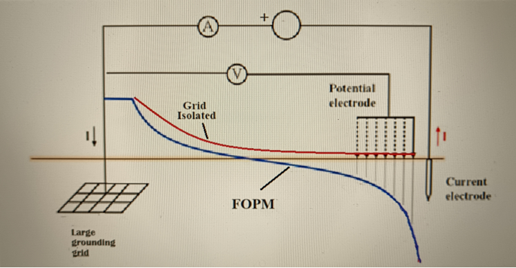
The three-pin method is represented in Figure 1. The electrode to be measured is connected to a distant auxiliary electrode through a current source with intensity I.

The circuit is completed through the ground. The potential difference between points A and B is

\begin{array}{l} V_{A} = V_{e} - \frac{ρ I}{2 π D} \\ V_{B} (x) = \frac{ρ I}{2 π x} - \frac{ρ I}{2 π (D - x)} \\ V_{A} - V_{B} (x) = V_{e} - \frac{ρ I}{2 π} (\frac{1}{D} + \frac{1}{x} - \frac{1}{D - x}) \end{array}

(1)

In expression (1),

V_{e}

is the potential of the electrode when it is isolated, i.e., the grounding potential. Additionally, it is implicitly assumed that at point x, both the grounding electrode and the auxiliary current electrode behave as point sources of current at ground level. The same applies to the auxiliary electrode with respect to point A. This question should be discussed in the case of long electrodes or not very large distances D.

Based on expression (1), the measured grounding resistance

R_{G}^{m e a s}

is defined as

R_{G}^{m e a s} (x) = \frac{V_{A} - V_{B} (x)}{I} = R_{G} - \frac{ρ}{2 π} (\frac{1}{D} + \frac{1}{x} - \frac{1}{D - x})

(2)

where

R_{G}

is the true grounding resistance. It is clear that

R_{G}^{m e a s} = R_{G}

for any given value of x, provided that the quantity in brackets in (2)

(\frac{1}{D} + \frac{1}{x} - \frac{1}{D - x}) = 0

is zero. Thus, solving for the value of x, it gives

x = 0.618 \cdot D

, known as the 62% rule, provided that the assumptions mentioned above are satisfied. In summary, by placing the auxiliary electrode at a sufficiently distant location D from the grounding point, this rule can be applied to obtain values that are very close to the true grounding resistance.

It is evident that the analysis presented here cannot be applied when measuring an extensive electrode or also when the distance D is not large enough to ensure that the potential generated by the auxiliary current electrode on the electrode to be measured is

\frac{ρ I}{2 π D}

as the implicit assumptions described above are no longer valid. An extensive mesh cannot behave like a point source of current unless viewed from an immensely large distance. It also cannot be applied if there is not enough space to place the auxiliary electrode sufficiently far away, even if the grounding system is not very extensive. Since the electrode can no longer be assimilated to a current point,

\begin{array}{l} V_{A} = V_{e} - \frac{ρ I}{2 π D} \\ V_{B} (x) = V_{e} (x) - \frac{ρ I}{2 π (D - x)} \\ V_{A} - V_{B} (x) = V_{e} - V_{e} (x) - \frac{ρ I}{2 π D} + \frac{ρ I}{2 π (D - x)} \end{array}

(3)

where

V_{e} (x)

is the potential created by the electrode at point x, considered as isolated and the distance D is not well defined since it must correspond to the distance at which V_A coincides with the true potential of the electrode. Dividing by the injected current I,

R_{G}^{m e a s} (x) = \frac{V_{A} - V_{B} (x)}{I} = R_{G} - \frac{V_{e} (x)}{I} + \frac{ρ}{2 π} (\frac{1}{D - x} - \frac{1}{D})

(4)

Note that from expression (4),

R_{G}^{m e a s} = R_{G}

, if and only if

V_{e} (x) = \frac{ρ I}{2 π} (\frac{1}{D - x} - \frac{1}{x})

for some value of x, otherwise will be above or below R_G depending on the value of x. This condition is equivalent to the 62% rule when it is not possible to assume that the electrode to be measured behaves as a current point. Next, the so-called correction factor

k_{m} (x)

will be introduced. It is defined as the ratio between the true grounding resistance and the resistance measured in the field

k_{m} (x) = \frac{R_{G}}{R_{G}^{m e a s} (x)}

. According to (4), it can be written as

k_{m} (x) = \frac{R_{G}}{R_{G} - \frac{V_{e} (x)}{I} + \frac{ρ}{2 π} (\frac{1}{D - x} - \frac{1}{D})} = \frac{k_{ρ}}{k_{ρ} - k_{p} (x) + \frac{1}{2 π} (\frac{1}{D - x} - \frac{1}{D})}

(5)

where the coefficients

k_{ρ} = \frac{R_{G}}{ρ}

and

k_{p} (x) = \frac{V_{e} (x)}{ρ I}

have been introduced. These coefficients

k_{ρ}

k_{p} (x)

turn out to be parameters of the electrodes and can be calculated for single-layered soils of resistivity

ρ

Therefore, the proposed method requires precise knowledge of the nature, geometry, and placement of the electrode, information that is presumably available, with which to evaluate

k_{ρ}

and

k_{p} (x)

. Once

k_{m} (x)

is obtained for a specific position of the potential probe, the electrode resistance

R_{G}^{m e a s} (x)

is measured, and the grounding resistance is found using

R_{G} = k_{m} (x) \cdot R_{G}^{m e a s} (x)

. Since these expressions have been derived from a drastic simplification, such as considering an extensive electrode as a point source at short distances, it is expected that

R_{G}

will depend on x and actually represent an upper bound to the true grounding resistance value. It should be noted that in the three-pin method, the measured resistance

R_{G}^{m e a s} (x)

is always lower than the real value.

As a comment, the denominator of (5) contains actually the touch potential of the electrode at distance x per unit of current and soil resistivity, known as

k_{c} (x)

and defined by

k_{c} (x) = \frac{V_{e} - V_{e} (x)}{ρ I}

, so (5) can also be expressed as

k_{m} (x) = \frac{k_{ρ}}{k_{c} (x) + \frac{1}{2 π} (\frac{1}{D - x} - \frac{1}{D})}

(6)

The magnitude

k_{c} (x)

can be evaluated theoretically, just like

k_{p} (x)

, given the nature, geometry, and positioning of the electrode in the soil. When dealing with extensive electrodes or with auxiliary current electrodes close to the electrode being measured, it becomes necessary to determine the appropriate value of D to use. It might be useful to rewrite (6) by introducing two distances,

k_{m} (x) = \frac{k_{ρ}}{k_{c} (x) + \frac{1}{2 π} (\frac{1}{D_{1} - x} - \frac{1}{D_{2}})}

(7)

where D₁ represents the distance between the auxiliary current electrode and the coordinate origin used to define the electrode being measured and D₂ is the optimal distance from the auxiliary electrode to the electrode being measured to obtain the potential V_A according to the first equation in (3). In critical situations, that is, when D₁ is not very large, we propose averaging R_G evaluated with two different values of D₂, corresponding to the nearest and farthest distances from the auxiliary electrode to the extensive electrode being measured. It is easy to see that

D_{1} \approx D_{2}

if both are large compared to the size of the electrode being measured so the point current approximation for the grounding electrode becomes quite accurate.

In the proposed method, we start with a known "theoretical" electrode for which it is possible to calculate

k_{c} (x)

k_{ρ}

and therefore

k_{m} (x)

according to (6). However, the electrode to be measured may not exactly correspond to the "theoretical" electrode. It may be altered for various reasons, so its resistance will not match the theoretical resistance. If we measure

R_{G}^{m e a s} (x)

, then applying the correction factor

k_{m} (x)

will not result in

R_{G}

. The main causes include oxidation or deterioration of the conductors that make up the electrode. Besides, the measurement can also be altered because the electrode is interconnected with other external grounds. This is a common practice that significantly reduces the resistance of the joint ground. With electrode deterioration the measure typically leads to grounding resistances

R_{G}^{m e a s} (x)

somewhat higher than those of the unaltered electrode, which, when multiplied by the correction factor, results in an overestimation of

R_{G}

. Thus, generally the result will be

R_{G} \leq k_{m} (x) \cdot R_{G}^{m e a s} (x)

. However, for interconnected electrodes, the measurement will give an underestimation of R_G. In either case, the proposed method will give the correct reading that corresponds to the case, and it is the task of the technical staff to determine the usefulness of the measurements. This hypothesis will be verified with the help of a numerical example in which a flat square electrode with a side length of 4 meters, made of conductive rods with a radius of 9mm, is buried at a depth of 0.5 meters. The soil is considered homogeneous with unitary resistivity. We are going to simulate the measurement of the grounding resistance by placing an auxiliary current rod 200 meters away from the electrode using the fall-of-potential method. For the same type of electrode, two situations will be addressed. In one case, the electrode has no issues, while in the other, it is assumed that part of the electrode is damaged and inactive in releasing current to the ground. Figure 2 shows the profiles of the electrode, and the dotted line represents the path traced to evaluate the potentials on the ground.

The difference of potential profile

V_{A} - V_{B} (x)

at points on the ground (z=0) along a straight line from the left side of the electrode at x=-2m to x=180m when the y-coordinate is fixed at y=2m, will be measured for both electrodes. Since the soil has a unit resistivity and the injected current is 1A, this potential difference represents the unit grounding resistance as a function of the distance x at which the potential probe is located, measured by the three-pin method, when the auxiliary electrode is, as previously mentioned, 200 meters from the electrode being measured.

Figure 3 shows the grounding resistance measured using the three-pin method, placing the potential electrode at distance x. The figure shows this measured resistance for both the original (red line) and the damaged electrode (beige line). The figure also shows the resistance corrected by the correction factor k_m, which is shown in the subfigure. The blue line is the result of this correction for the original electrode. As seen, the value R_G = 0.1114 Ω corresponding to the true resistance of the original electrode is obtained. In contrast, for the damaged electrode, applying the correction factor results in an R_G value above the true resistance value, which is 0.1266 Ω. Note that the correction factor is derived from the original electrode parameters and is applied to all situations, whether the electrode is damaged or not.

3. Application to Real Cases for Validation of the Method

The method described in the previous section will be applied to two real large electrodes. In the first case, the field measurement of the grounding resistance using the three-pin method will be simulated. In the second case, the resistance of the electrode is obtained from real field data.

3.1. Grounding Grid of the Balaidos Substation

The method described in the previous section will be applied to determine the grounding resistance of an extensive electrode, such as the grounding grid of the Balaidos substation in Vigo, Galicia, Spain. The technical characteristics of the mesh are cited below. Specifically, the resistance of the grounding electrode of the Balaidos electrical substation belonging to the Electric Company Unión Fenosa, located in Vigo, Galician Community (Spain), will be estimated. Figure 4 shows the geometric structure of the electrode, which is a non-regular grid formed by rods of variable length.

The electrode of 4 mm radius is buried at a depth of 0.8 m and the parameter

k_{R} = \frac{R_{G}}{ρ}

is previously known. The value is k_ρ=0.02766 Ω/Ωm, which represents the unitary grounding resistance provided that ρ=1 Ωm. The measurement using the three-pin method is simulated with the help of an auxiliary current electrode at a distance of 300 meters from the long edge of the mesh. Given the large distance between the auxiliary electrode and the grounding grid, we will assume

D_{1} \approx D_{2} = 300

m in (7). The soil is considered to be a single layer with unit resistivity, and the current injected into the mesh-auxiliary electrode circuit is 1 ampere. The absolute potential generated by the isolated mesh in the surrounding area can be simulated. Specifically, considering the dashed path drawn in the subfigure of Figure 5, the absolute potential at points along this path is shown.

Figure 6 shows the variation of the measured resistance

R_{G}^{m e a s} (x)

(blue line) with the coordinate x from the edge of the mesh, as well as the correction factor

k_{m} (x)

corresponding to the single grid and theoretically calculated (subfigure blue line). The product

R_{G} = k_{m} (x) \cdot R_{G}^{m e a s} (x)

is shown (red line), which ideally represents the true grounding resistance of the electrode obtained from the measurement at distance x. It can be observed that

R_{G}

is almost everywhere constant and equals the true grounding resistance value R_G=0.02766 Ω.

Figure 6 also illustrates the situation where the Balaidos grid is interconnected with another distant grid that is part of an external grounding system. In this case, a fault either in Balaidos or in the distant installation causes both grounding systems to act as one. The figure shows the field measurement of the combined grounding (beige line), while the magenta line represents the product of this measured resistance by the correction factor k_m from Balaidos grid as isolated. The result is an almost constant graph, which is also equal to the grounding resistance of the interconnection. In this case, R_G = 0.01912 Ω, which is 3% lower than the theoretical value of the combined grounding system R_G=0.01963 Ω.

3.2. Grounding Grid of the Loeches Substation

Loeches is a large substation located in Loeches (Madrid), with approximate dimensions of 350 meters in length by 250 meters in width. The substation, owned by Union Fenosa Distribucion (UDF), has voltage levels of 132 kV, 45 kV, and 15 kV, and is located next to another large substation owned by Red Eléctrica de España, with a voltage level of 220 kV. In Figure 7, the 45 kV/15kV section of the UFD substation is outlined in red.

The auxiliar current electrode used, consisting of 4 copper rods connected in parallel and spaced approximately 2 meters apart, was installed at a distance of about 100 meters from the substation perimeter fence (green dot). In Figure 7, the position of the auxiliary current electrode is shown as a blue dot. To measure the substation grounding resistance, an auxiliary voltage electrode was used, consisting of a rod driven into the ground at an approximate distance of 40 meters from the substation perimeter fence, in the direction of the current electrode.

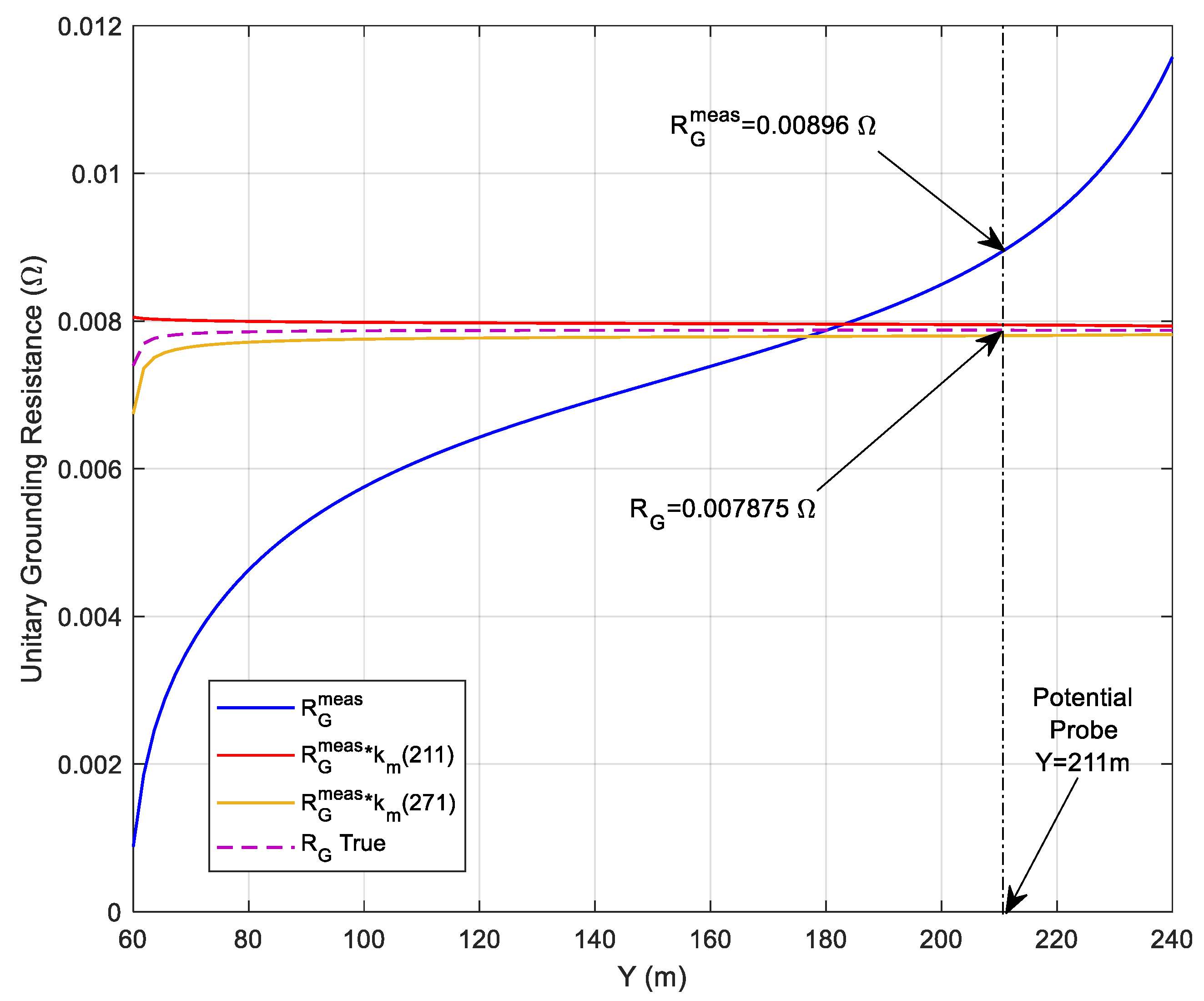
Based on the technical data of the grounding electrode shown in the right panel of Figure 7, it is easy to calculate and

k_{ρ} = 0 . 00787

Ω/Ωm and

k_{c} (x)

, along the yellow line shown in Figure 7, to finally evaluate

k_{m} (x)

according to (7). For this final step, D₁=271 m, and D₂ will take two values, 271 meters and 211 meters from the auxiliary electrode, since the coordinate origin on the ground is the point (X0 = 35 m, Y0 = 0). With respect to this coordinate origin, the potential probe is located at the point with coordinates (X_p = 35 m, Y_o = 211 m, Z_p = 0).

Figure 8 shows the results of the analysis. The solid blue line represents, as in previous examples, the field measurement values of the electrode resistance using the FOPM

R_{G}^{m e a s} (x)

. These values are expressed as unit resistance, knowing that the estimated soil resistivity is ρ= 59.5 Ωm. The solid red and beige lines represent the corrected values of

R_{G}^{m e a s} (x)

using the correction coefficient k_m evaluated with D2 = 211 m and D2 = 271 m, respectively and D1=271 m, according to (7). Finally, the magenta dashed line shows the average of both corrections, corresponding to the estimated resistance of the electrode. The figure also shows the value measured by the potential probe 40 meters from the perimeter fence, which corresponds to a distance of 211 m from the coordinate origin. As can be seen in the figure, the estimated value for the grounding resistance, obtained by correcting the field-measured values at any distance from the potential probe, is constant and has a value of R_G= 0.007875 Ω, in full agreement with the theoretical value associated with the electrode.

4. Conclusions

Field measurement of the grounding resistance of large electrodes presents practical problems that are not easily solved. The commonly used three-pin method requires that the return electrode be sufficiently separated from the electrode to be measured so that it can be considered a current point, and the well-known 62% rule can be applied. Otherwise, the potential provided by the three-pin arrangement must be properly corrected. This paper proposes a simple method to correct the reading obtained from the direct measurement to obtain the actual grounding resistance. However, the value given by the method may not correspond to the theoretical value of the electrode due to various causes such as deterioration or interconnection with other groundings. In any case, the value given by the correction to the field measurements provides the correct value that would be obtained by applying the fall-of-potential method to a three-pin scheme with the auxiliary current electrode sufficiently far away, if this could be carried out. Such an auxiliary current electrode can be located at a relatively close distance to the electrode to be measured and the potential probe can be placed at any intermediate distance. The only requirement is that the electrode is known in all its physical characteristics as well as its location in the ground with known resistivity.

Author Contributions

Jorge Moreno (JM), Eduardo Faleiro (EF), Daniel Gracia (DG), Pascual Simon (PS), Gregorio Denche (GD) and Gabriel Asensio (GA). Conceptualization, JM, EF and PS.; methodology, JM, EF,DG and PS.; software, DG, GD and GA.; validation, JM,EF,PS and DG; formal analysis, JM,EF,DG and PS.; investigation, JM, EF and PS; resources, DG, PS, GD and GA; data curation, PS, GD and GA; writing—original draft preparation, JM, EF, PS, GD and GA; writing—review and editing, JM, EF, GD and GA; visualization, JM and EF.; supervision, JM and EF.; project administration, JM and EF. All authors have read and agreed to the published version of the manuscript.

Funding

This research received no external funding.

Institutional Review Board Statement

Not applicable.

Data Availability Statement

The data used in this paper are not public but has been kindly provided by the company Union Fenosa Distribucion S.A.

Acknowledgments

The authors would like to thank both the Department of Applied Mathematics and the IEEF Department of the Escuela Técnica Superior de Ingeniería y Diseño Industrial (ETSIDI) at the Universidad Politecnica de Madrid (UPM) for their support to the undertaking of the research summarized here. Furthermore, the authors appreciate the collaboration with the firm QUIBAC at Terrassa, Barcelona (Spain), for the technical support. Finally, we also would like to thank for the support provided by Unión Fenosa Distribución S.A. for allowing the use of data from electrical installations for scientific purposes to perform this work.

Conflicts of Interest

The authors declare no conflict of interest.

References

Zhiwei, L.; Zhao, Z. The Grounding Impedance Calculation of Large Steel Grounding Grid. 2012 International Conference on Future Electrical Power and Energy Systems. Energy Procedia 2012, 17, 157–163. [Google Scholar] [CrossRef]
Freschi, F.; Mitolo, M.; Tartaglia, M. An Effective Semianalytical Method for Simulating Grounding Grids. IEEE Trans. Ind. Appl. 2013, 49, 256–263. [Google Scholar] [CrossRef]
Trifunovic, J.; Kostic, M.B. An Algorithm for Estimating the Grounding Resistance of Complex Grounding Systems Including Contact Resistance. IEEE Trans. Ind. Appl. 2015, 51, 5167–5174. [Google Scholar] [CrossRef]
Denche, G.; Faleiro, E.; Asensio, G.; Moreno, J. An Estimator of the Resistance of Large Grounding Electrodes from Its Geometric Characterization. Appl. Sci. 2020, 10, 8162. [Google Scholar] [CrossRef]
Korasli, C. Ground Resistance Measurement with Alternative Fall-of-Potential Method. 2005/2006 IEEE/PES Transmission and Distribution Conference and Exhibition. [CrossRef]
IEEE Guide for Measuring Earth Resistivity, Ground Impedance, and Earth Surface Potentials of a Ground System, IEEE Std. 81-2012,2012.
Ladanyi, J.; Smohai, B. Influence of Auxiliary Electrode Arrangements on Earth Resistance Measurement Using the Fall-of-Potential Method. 2013 4th International Youth Conference on Energy (IYCE). [CrossRef]
Dimcev, V.; Handjiski, B.; Vrangalov, P.; Sekerinska, R. Vrangalov, R. Sekerinska. Impedance measurement of grounding systems with alternative fall-of-potential method. Conference Record of the 2000 IEEE Industry Applications Conference. Thirty-Fifth IAS Annual Meeting and World Conference on Industrial Applications of Electrical Energy (Cat. No.00CH37129). [CrossRef]
Alcantara, F.R. An Approximated Procedure to Find the Correct Measurement Point in the Fall-of-Potential Method. 2018 IEEE PES Transmission & Distribution Conference and Exhibition - Latin America (T&D-LA). [CrossRef]
Nassereddine, M.; Rizk, J.; Nagrial, M.; Hellany, A. Substation earth grid measurement using the fall of potential method (FOP) for a limited test area. 2014 Australasian Universities Power Engineering Conference (AUPEC). [CrossRef]
Wang, C.-G.; Takasima, T.; Sakuta, T.; Tsubota, Y. Grounding resistance measurement using fall-of-potential method with potential probe located in opposite direction to the current probe. IEEE Trans. Power Deliv. 1998, 13, 1128–1135. [Google Scholar] [CrossRef]
Huang, H.; Liu, H.; Luo, H.; Du, H.; Xing, Y.; Li, Y.; Dawalibi, F.P.; Zhou, H.; Fu, L. Analysis of a Large Grounding System and Subsequent Field Test Validation Using the Fall of Potential Method. Energy Power Eng. 2013, 5, 1266–1272. [Google Scholar] [CrossRef]
Yuan, T.; Bai, Y.; Sima, W.; Xian, C.; Peng, Q.; Guo, R. Grounding Resistance Measurement Method Based on the Fall of Potential Curve Test Near Current Electrode. IEEE Trans. Power Deliv. 2016, 32, 2005–2012. [Google Scholar] [CrossRef]
Colella, P.; Pons, E.; Tommasini, R.; Di Silvestre, M.L.; Sanseverino, E.R.; Zizzo, G. Fall of Potential Measurement of the Earth Resistance in Urban Environments: Accuracy Evaluation. IEEE Trans. Ind. Appl. 2019, 55, 2337–2346. [Google Scholar] [CrossRef]
SIST EN 50522:2022 - Earthing of power installations exceeding 1 kV a.c.

Figure 1. Practical illustration of the Three-Pin method for measuring the grounding resistance R_G.

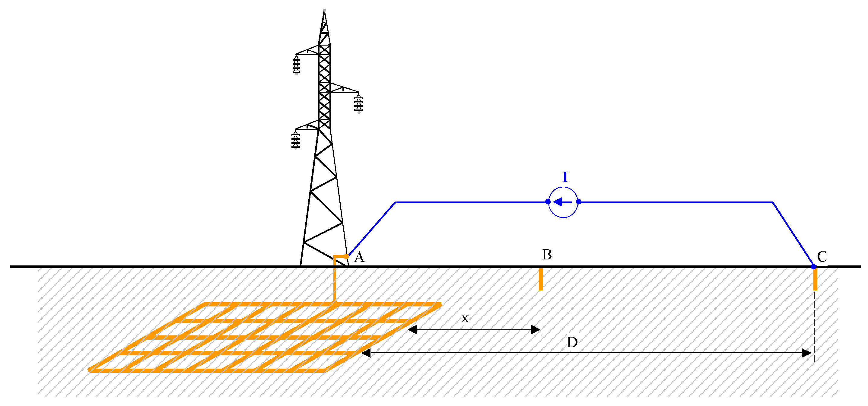
Figure 2. The upper panel shows the electrode being studied, while the lower panel represents the same electrode partially damaged.

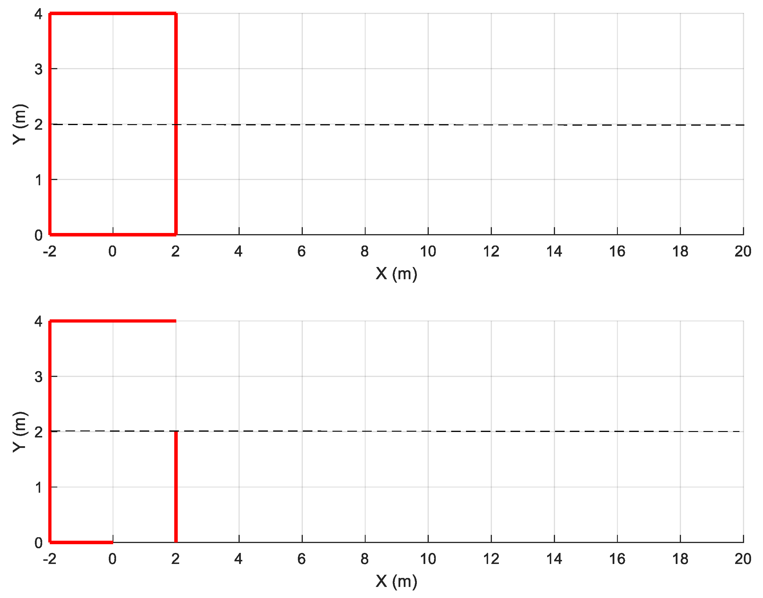
Figure 3. The measured grounding resistance profile for the original electrode (red line) and for the damaged electrode (beige line).

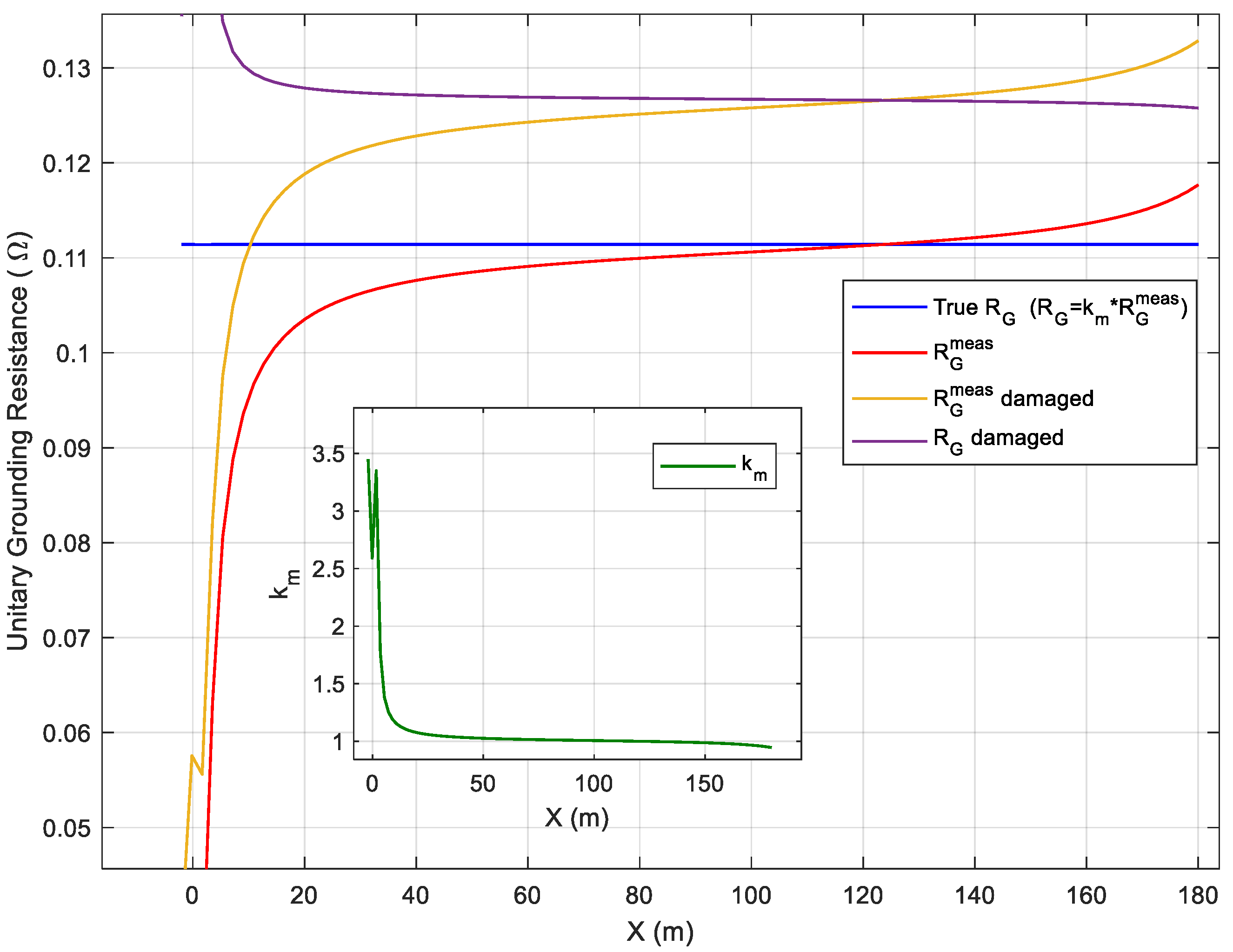
Figure 4. The Balaidos substation grounding grid.

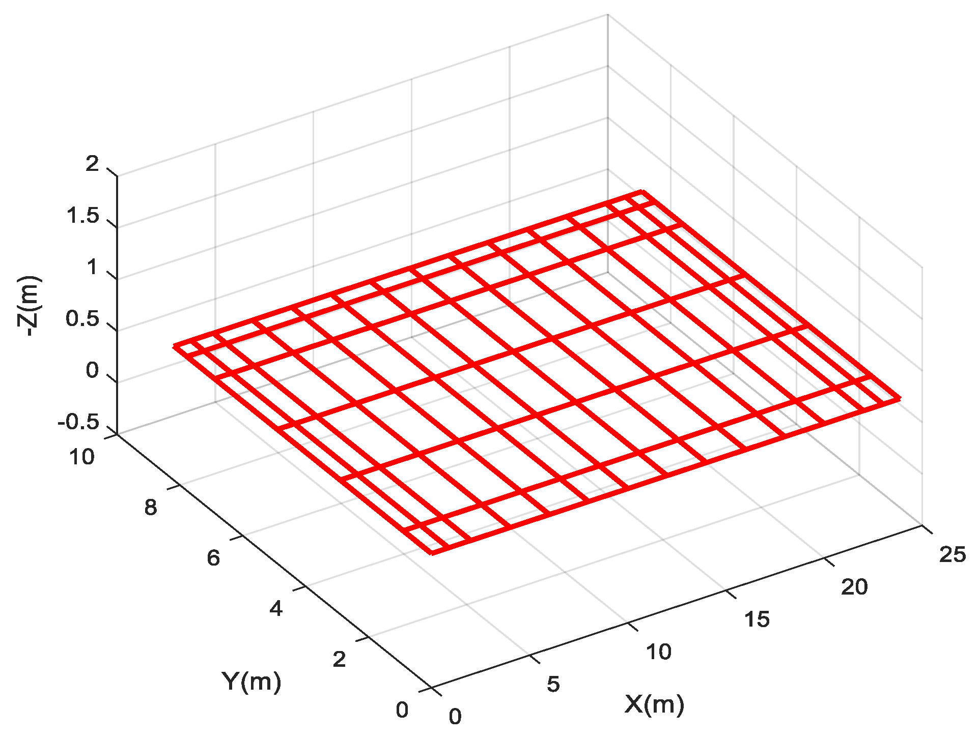
Figure 5. Balaidos grid with the indicative line on the ground where the absolute potential is measured by the three-pin method (blue line) when auxiliar rod is 300 m far away. The absolute potential created by the isolated grid is also shown (red line).

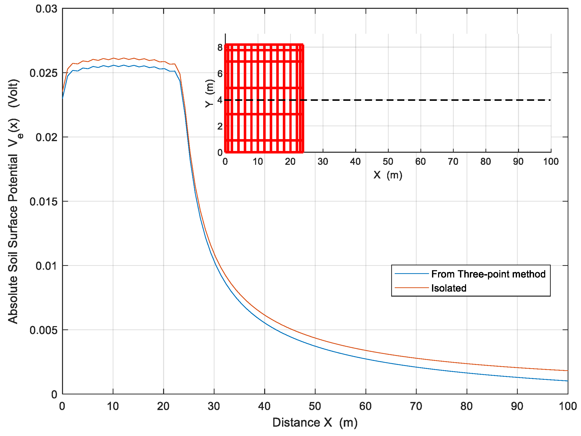
Figure 6. Representation of the different measurement procedure parameters as a function of the distance from the edge of the Balaidos grid. An interconnected case with other grounding system is also considered.

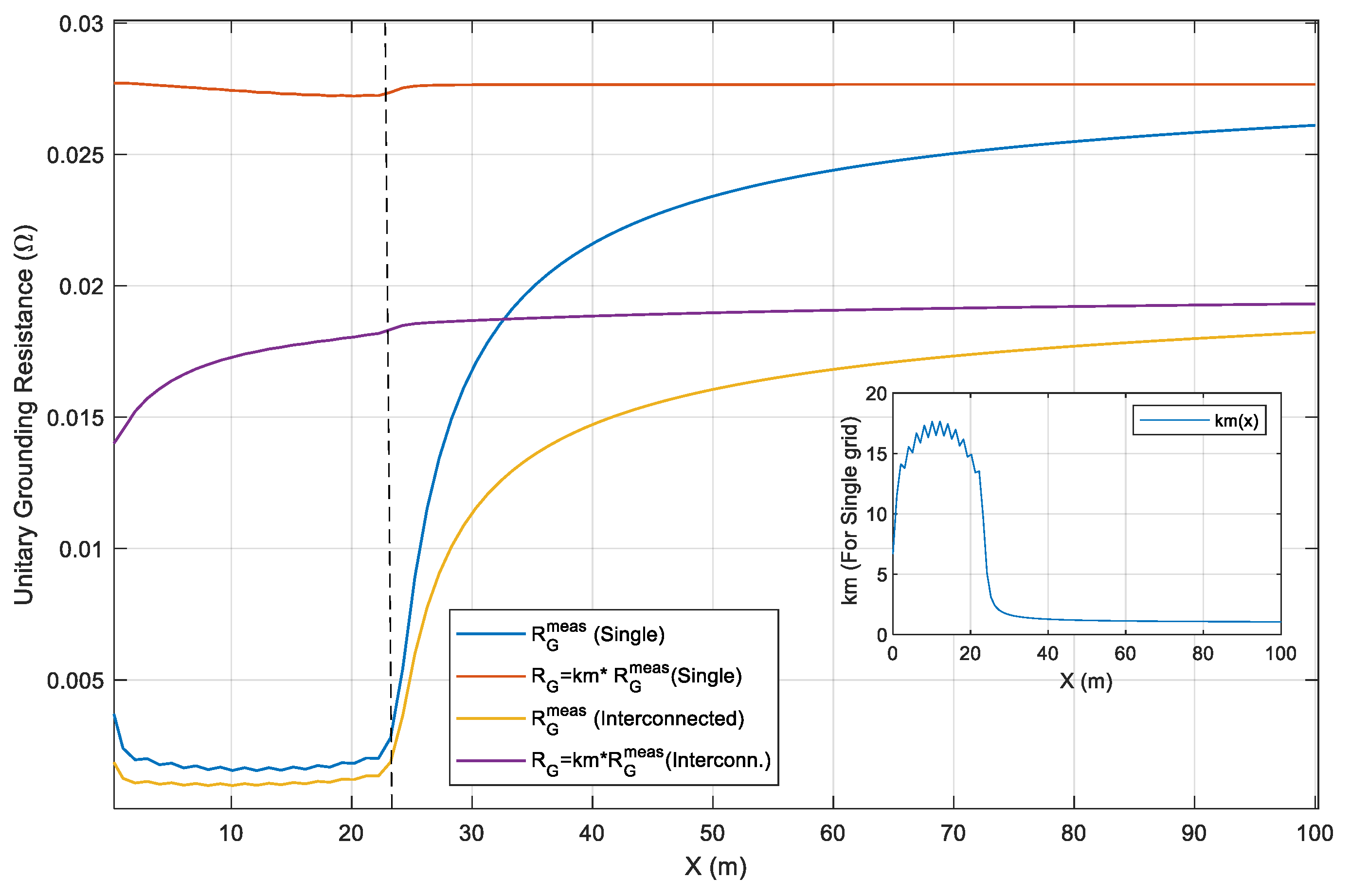
Figure 7. In the left panel, the Loeches substation, marked in red. The blue dot is the auxiliary current electrode 211 meters away from the grid edge. (Courtesy of Union Fenosa Distribucion, UFD). The grounding grid is shown on the right panel.

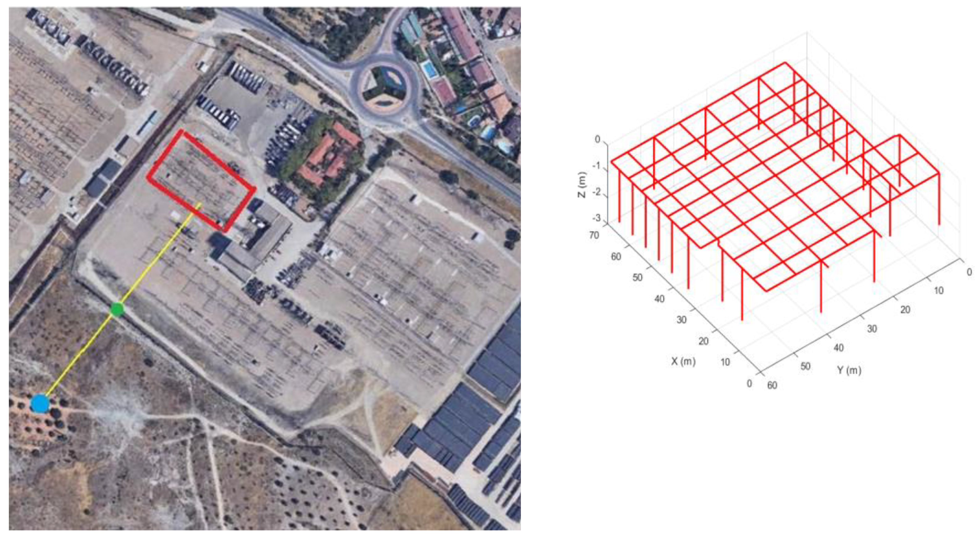
Figure 8. The different unitary resistances associated with the studied case, as discussed in the text.

Disclaimer/Publisher’s Note: The statements, opinions and data contained in all publications are solely those of the individual author(s) and contributor(s) and not of MDPI and/or the editor(s). MDPI and/or the editor(s) disclaim responsibility for any injury to people or property resulting from any ideas, methods, instructions or products referred to in the content.

© 2024 by the authors. Licensee MDPI, Basel, Switzerland. This article is an open access article distributed under the terms and conditions of the Creative Commons Attribution (CC BY) license (http://creativecommons.org/licenses/by/4.0/).

Copyright: This open access article is published under a Creative Commons CC BY 4.0 license, which permit the free download, distribution, and reuse, provided that the author and preprint are cited in any reuse.

Downloads

Views

Comments

Subscription

Notify me about updates to this article or when a peer-reviewed version is published.

MDPI Initiatives

Important Links

Choose an area of interest and we will send you notifications of new preprints at your preferred frequency.

Disclaimer