1. Introduction
Weather prediction is essential for various sectors, including agriculture, infrastructure, and disaster management. However, Numerical weather prediction models, as for instance those used by the European Center for Medium-Range Weather Forecasts (ECMWF), and GCMs often have coarse resolutions, making them insufficient for local-scale applications. These models simulate Earth’s climate by integrating atmospheric, oceanic, and land surface processes and use data assimilation to enhance forecast accuracy. To address the limitations of NWPs and GCMs, downscaling techniques refine the outputs of these models to generate high-resolution climate data, providing detailed local insights. This refinement is crucial for accurate, actionable climate forecasts tailored to specific regions. [
1,
2,
3]. Downscaling methods transform large-scale climate information into finer scales, which are crucial for accurately predicting local/regional climate impacts [
4].
Traditional downscaling methods include statistical and dynamical approaches. Statistical downscaling relies on historical data to establish relationships between large-scale and local-scale climate variables, providing a straightforward method for refining NWP and GCM outputs. Dynamical downscaling, on the other hand, employs high-resolution regional climate models (RCMs) to simulate local climate with greater accuracy by incorporating finer-scale physical processes [
5,
6,
7,
8].
For instance, [
2] developed a statistical downscaling method that combines the optimum correlation method (OCM) and Bayesian model averaging (BMA) to enhance precipitation predictions in China. This method effectively improved forecast accuracy by leveraging historical climate data. Similarly, [
9] utilized a Non-Homogeneous Hidden Markov Model (NHMM) to downscale daily rainfall, successfully linking large-scale meteorological features to local rainfall patterns and accurately simulating rainfall seasonality and extremes. Additionally, [
10] proposed a new hierarchical model that significantly improved the NHMM’s accuracy in simulating spatiotemporal precipitation features, particularly for extreme precipitation events. These examples demonstrate the diverse applications and benefits of traditional downscaling techniques in improving climate predictions at local scales.
Recently, deep learning (DL) models have emerged as powerful tools for downscaling due to their ability to learn complex nonlinear relationships in spatiotemporal data. [
11] introduced DeepSD, a generalized stacked super-resolution convolutional neural network (SRCNN) framework for statistical downscaling of climate variables, demonstrating significant improvements over traditional approaches. Moreover, [
5] applied convolutional-based downscaling models to visualize and understand the implicit feature selection within neural networks, proving their potential in connecting large-scale and local-scale climate patterns.
A significant development in the field of deep learning for image processing is the Generative Adversarial Network (GAN), introduced by [
12]. GANs use a generator-discriminator framework, where the generator attempts to produce realistic images, and the discriminator aims to differentiate between real and generated images. Building on this concept, [
13] developed the Super-Resolution Generative Adversarial Network (SRGAN), which is capable of generating realistic textures in single image super-resolution by learning a mapping from low-resolution to high-resolution images. SRGAN has shown remarkable ability in enhancing image details, making it a valuable tool for applications requiring high-resolution outputs.
Despite these advances, DL-based downscaling models often suffer from artifacts and biases, especially when applied to climate data with complex terrain and extreme weather events. [
14] addressed these issues by applying the SRGAN to climate prediction, using a perceptual loss function to recover high-frequency details in generated high-resolution images. However, even SRGAN models can produce artifacts, as noted by [
15], who proposed DeepDT, a model that further eliminates artifacts by training a generator and discriminator separately and using a residual-in-residual dense block structure.
Incorporating auxiliary inputs such as elevation maps can significantly enhance the accuracy and reliability of downscaling models. Elevation plays a crucial role in influencing local climate variables, particularly precipitation and temperature [
16]. For example, [
16] combined ERA5 reanalysis data [
17,
18] with high-resolution simulations using a CNN-based model to downscale precipitation in the Tibetan Plateau, achieving lower biases and higher accuracy compared to traditional methods. Similarly, [
19] developed a deep convolutional neural network with skip connections and attention blocks to downscale precipitation data in Taiwan, demonstrating superior performance over other methods.
Our study builds on these advancements by introducing Elevation-Integrated Temperature and Precipitation SRGAN Downscaling (E-TEPS), an SRGAN-based model that integrates elevation maps as an auxiliary input to improve the downscaling of temperature and total precipitation variables. This research utilizes Google Cloud for preprocessing, data downloading, training, and inference, leveraging cutting-edge hardware and GPUs to handle the computational demands efficiently. The initial work for this project began with a GitHub repository (
https://github.com/mantariksh/231n_downscaling), which provided a foundational codebase. This code was extensively modified and enhanced to develop E-TEPS, a novel downscaling SRGAN model tailored to our specific needs. The modifications included architectural changes to the model, optimization of training processes, and incorporation of new techniques to enhance the model’s performance.
A key novelty of our work is the integration of elevation maps into our model. Elevation plays a critical role in influencing local climate variables, particularly precipitation and temperature, which can vary significantly with altitude. By including elevation as an auxiliary input, our model captures these variations more accurately, leading to improved downscaling performance.
The loss functions used in our model are designed to ensure both the adversarial and content aspects of the generated images are optimized. The discriminator loss employs a Binary Cross-Entropy with Logits Loss (BCEWithLogitsLoss) to distinguish between real and generated images effectively. The generator loss combines a Mean Squared Error (MSE) content loss with an adversarial loss, weighted to balance the reconstruction fidelity and adversarial realism. This approach is similar to, but extends beyond, the methods used in previous works, such as those by [
14] and [
13], by incorporating elevation data and fine-tuning the loss parameters for better performance.
To validate our model, we compare its outputs against traditional downscaling models such as bicubic and bilinear interpolation. These conventional methods, while straightforward, often fail to capture the complex spatial patterns and fine details that our enhanced model can reproduce. Our results demonstrate significant improvements in key metrics such as Mean Absolute Error (MAE), Root Mean Square Error (RMSE), Pearson Correlation for temperature, agreement analysis for total precipitation, and also visual comparison between the generated images and true high resolution images showcasing the superior accuracy and visual quality of our downscaled climate predictions.
The remainder of this paper is structured as follows: We begin with a review of related work in climate downscaling and deep learning, discussing various techniques and their applications. We then detail the methodology of E-TEPS, including the integration of elevation maps and the specific architecture used. Following this, we present the experimental setup and results, comparing our model’s performance with other state-of-the-art methods. We also discuss the implications of our findings, highlighting the potential for future research and applications in different regions and climates. Finally, we conclude with a summary of our contributions and key results.
2. Materials and Methods
2.1. Dataset
2.1.1. Training Data
The dataset used in this study is derived from dynamically downscaling ERA5 reanalysis data, originally at a resolution of 31 km, to a high spatial resolution of 2.2 km [
20]. It covers the entire Italian territory and neighboring regions, extending from a latitude of 34.8 to a longitude of 3.91. The dataset spans from January 1989 to December 2020, with an hourly temporal resolution.
We chose this dataset because of its high spatial resolution and structural similarity to the ERA5 data make it ideal for training E-TEPS. These characteristics enable the model to produce accurate and detailed climate forecasts, essential for enhancing early-warning systems [
21].
The specific data used to train the model includes 2-meter temperature above the surface and total precipitation. The training period covers from January 1, 1998, to December 31, 2018, while the validation period spans from January 1, 2019, to December 31, 2021. Additionally, data from the year 2022 is used for testing and inference the trained model. The temporal resolution for all datasets is 6 hours, with data points collected at 00, 06, 12, and 18 hours each day. This selection helps reduce the training data size, aligns with the structure of cutting-edge forecasting models like FourCastNet [
22] and GraphCast [
23], and covers more years of data. For precipitation, a 6-hour accumulation is performed, meaning the total precipitation value at 12:00, for example, is the sum of precipitation from 07:00 to 12:00 on the same day.
2.1.2. Elevation Map
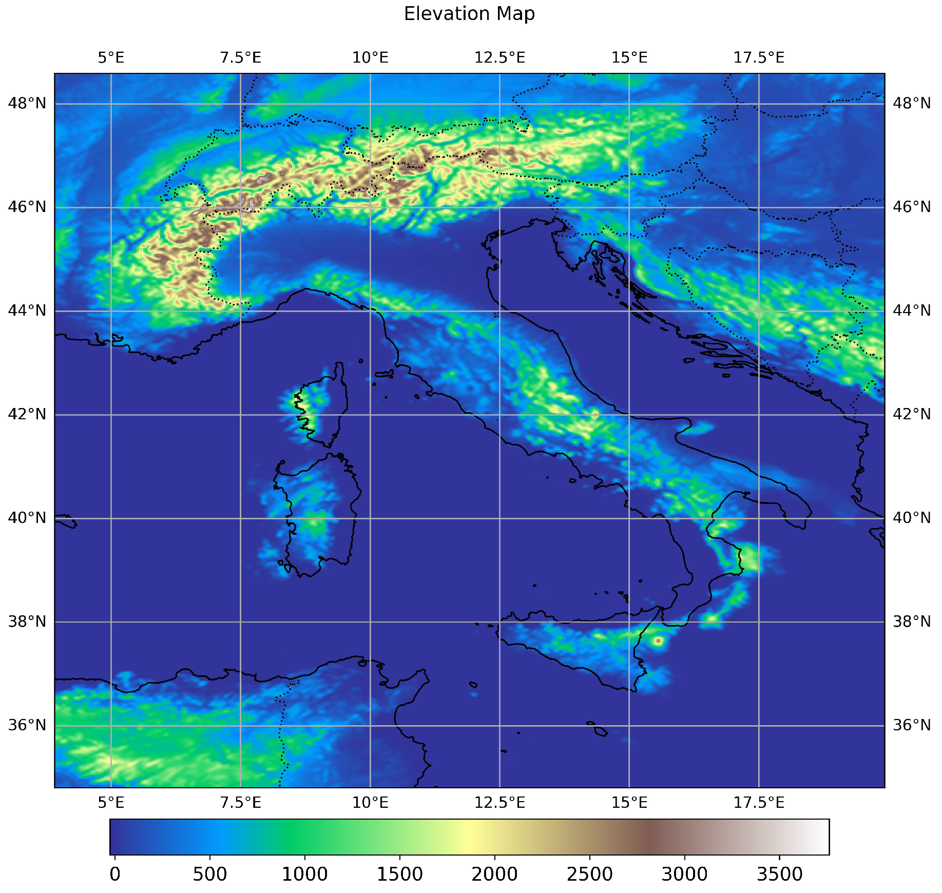
The elevation map, as shown in
Figure 1, is utilized throughout all steps of the model, from training to inference. This map has been downloaded from the same database as the other climate variables and shares the same high spatial resolution of 2.2 km. It is used as an auxiliary input channel in the model to enhance the accuracy of the downscaling method.
2.2. Preprocessing of the Data
The preprocessing method used to upscale the original dataset involves several key steps. First, the data is smoothed using a Gaussian filter, which helps in reducing noise and making the data more uniform. The smoothed data is then downsampled to a lower resolution using the Bivariate spline approximation over a rectangular mesh (RectBivariateSpline) method. This method creates a new dataset with reduced resolution by mapping the original high-resolution data to a specified lower resolution grid. Additionally, a threshold function is applied to the precipitation data to ensure no negative values are present. This preprocessing is done for both temperature and precipitation data.
The reason for this preprocessing is to train the model to downscale low-resolution datasets by a factor of eight. The goal is to achieve a low-resolution dataset with a resolution similar to the ERA5 dataset, which is approximately 30 km. To facilitate this, the original high-resolution data at 2.2 km resolution is converted to a coarser resolution of around 3.475 km. This allows the model to be trained on a dataset that mimics the ERA5 resolution, enabling it to learn how to effectively downscale to high-resolution outputs from low-resolution inputs.
2.3. Training
2.3.1. DataLoader Configuration
The data preparation for training the model involves loading and processing elevation, precipitation, and temperature data. Elevation data is normalized and interpolated to ensure consistency in resolution with the other variables. Precipitation and temperature data are retrieved and subjected to smoothing using a Gaussian filter to reduce noise.
2.3.2. Normalization and Scaling
The smoothed precipitation and temperature data are downsampled to create lower-resolution inputs that mimic the ERA5 dataset’s resolution of approximately 30 km. These downsampled data are normalized to have zero mean and unit variance and then scaled to a range of [-1, 1]. This scaling aligns with the use of the hyperbolic tangent (tanh) activation function in the generator architecture of the model, ensuring that the data fed into the model are within the appropriate range for effective learning.
2.3.3. Dataset Statistics
Statistics such as mean and standard deviation are computed for both precipitation and temperature data. These statistics are essential for normalization, ensuring that the training and validation data are on a similar scale. The computed statistics are saved and reloaded as needed to maintain consistency across different training sessions.
2.3.4. Loss Functions and Optimizers
The discriminator loss function aims to distinguish between real and generated images. It uses the Binary Cross Entropy with Logits Loss. The loss is computed by comparing the discriminator’s predictions on real images to a set of labels indicating real images and its predictions on generated images to a set of labels indicating fake images. The total loss is the sum of the losses from these two comparisons, as shown in Equations
1,
2, and
3. This approach is described in the work by [
13,
24], and [
25].
The generator loss function combines content loss and adversarial loss to ensure the generated images are both perceptually similar to the true images and convincing to the discriminator. The content loss, measured by Mean Squared Error (MSELoss), ensures the generated images closely match the true high-resolution images. The adversarial loss computed using
BCEWithLogitsLoss, that combines the logistic sigmoid activation and binary cross-entropy loss and ideal for binary classification tasks with logits as output, encourages the generator to produce images that the discriminator classifies as real. These two components are weighted and summed to form the total generator loss, as shown in Equations
4,
5, and
6.
where
is a weight parameter.
The model optimization is handled using the AdamW optimizer, a variant of the Adam optimizer with weight decay to improve regularization. This optimizer is configured with specific learning rates and momentum parameters to ensure stable and efficient convergence of the model during training[
13,
24,
26].
2.3.5. Network Architectures
Discriminator Architecture: The discriminator network is designed to distinguish between real and generated high-resolution images. It employs a series of convolutional layers with increasing depth, interspersed with Leaky ReLU activations and batch normalization to stabilize training and improve convergence. The network starts with a convolutional layer that processes the input channels and extracts features. As the data passes through subsequent layers, the spatial resolution is progressively reduced through strided convolutions, allowing the network to capture hierarchical features at different scales. The final layers flatten the output and use fully connected layers to produce a single scalar value, which indicates the probability of the input being a real high-resolution image.
Key components of the discriminator include:
Convolutional Layers: Extract features from the input images.
Leaky ReLU Activations: Introduce non-linearity and help in learning complex patterns.
Batch Normalization: Stabilize and accelerate training.
Fully Connected Layers: Combine extracted features to make a final binary decision.
Generator Architecture: The generator network is responsible for converting low-resolution images to high-resolution outputs. It begins with an initial convolutional layer followed by a series of residual blocks. These residual blocks help in learning the identity mappings and retaining the input information, which is crucial for generating high-quality images. Each residual block contains convolutional layers, batch normalization, and PReLU activations. After the residual blocks, the network includes a post-residual convolutional layer to further refine the features.
To downscale the image to the desired high resolution, the generator uses a combination of convolutional layers and pixel shuffle operations, which rearrange the elements of the convolutional outputs to increase the spatial resolution. The final convolutional layers produce the output image, which is activated using the tanh function to ensure the pixel values are within the range of [-1, 1].
Key components of the generator include:
Initial Convolutional Layer: Prepares the input for further processing.
Residual Blocks: Enhance feature extraction while preserving input information.
Post-Residual Convolutional Layer: Refines the features before upscaling.
Pixel Shuffle Operation: Efficiently increases the spatial resolution.
Final Convolutional Layer and Tanh Activation: Produce the final high-resolution image output.
This architecture enables the generator to effectively learn the mapping from low-resolution to high-resolution images, providing detailed and accurate outputs suitable for enhancing the resolution of climate forecast data.
2.3.6. Training Loop
The training loop iteratively updates both the generator and discriminator networks to produce high-resolution outputs from low-resolution inputs. Each epoch consists of processing batches of data, where the discriminator distinguishes between real high-resolution images and those generated by the generator. The discriminator is updated based on its ability to differentiate these images, while the generator is updated to improve its ability to produce realistic high-resolution images. This involves computing and back-propagating the respective loss functions for both networks.
To enhance training efficiency and stability, gradient accumulation is used, where gradients are accumulated over multiple iterations before performing an optimizer step. Mixed precision training with automatic mixed precision (AMP) is employed to speed up training and reduce memory usage. Throughout the training process, metrics such as discriminator and generator losses are logged, and periodic evaluations on a validation set are conducted to monitor performance.
2.4. Inference
For the inference stage the model is used to downscale low-resolution climate data to high-resolution outputs. The input data for inference already has a low resolution matching the training data’s low-resolution scale, so no further upscaling is required. The preprocessing steps for the elevation data are identical to those used during training, ensuring consistency in the input variables. Normalization and scaling are also applied using the statistics saved during the training phase, aligning the input data within the expected range of the model.
The network architecture for the generator remains the same as used during training. During inference, the low-resolution input data, along with the normalized and interpolated elevation data, are fed into the generator model. The generator produces high-resolution outputs, which are then denormalized using the stored statistics from the training phase. For precipitation data, a reverse log transformation is applied to obtain the final high-resolution predictions.
The inference loop involves processing each input sample through the generator model, storing the output, and applying necessary post-processing steps such as denormalization and reverse log transformation. This loop continues for all time steps in the dataset, ensuring that the model generates high-quality, high-resolution climate predictions consistent with the training and validation phases. This process leverages the robust hardware setup and optimized model architecture to efficiently downscale low-resolution climate data to detailed, high-resolution outputs.
2.5. Hardware and Computational Resources
The training and computational processes for this study were conducted using Google Colab and cloud services. Specifically, the NVIDIA GeForce A100 GPU available through Google Colab Pro Plus was utilized. This setup provided 40GB of GPU RAM and 80GB of system RAM, which was essential for handling the computational demands of training the model. The total size of the training data was approximately 40GB, necessitating the robust hardware capabilities offered by this platform.
3. Results and Discussion
In this section, we present and discuss the performance of our model in comparison to traditional bicubic and bilinear interpolation methods. The evaluation is based on key metrics such as Mean Absolute Error (MAE), Root Mean Squared Error (RMSE), Agreement Analysis, and Pearson Correlation. Additionally, we provide a visual comparison of downscaled images for selected timesteps across different seasons.
The datasets used in this study include generated images produced by our model during the inference phase, as well as bicubic and bilinear interpolations of low-resolution images downscaled to the same resolution as the high-resolution images generated by our model. These high-resolution images are compared against ground truth high-resolution images in a detailed evaluation. The datasets contain two primary climate variables: accumulated total precipitation, measured in millimeters (mm), and 2m temperature above the surface, measured in Kelvin (K), both with a 6-hour temporal resolution.
The comparison approach involves quantitative analysis, agreement analysis, Pearson correlation, and visualization analysis, which collectively highlight the performance of each method against the ground truth data. All analyses are conducted using their units. MAE measures the average magnitude of the errors between the predicted and observed values, without considering their direction. It is calculated as shown in Equation (
7). A lower MAE indicates a better fit of the model to the data. RMSE provides a measure of the differences between predicted and observed values. It is the square root of the average of squared differences, as given in Equation (
8). RMSE gives higher weight to larger errors, making it more sensitive to outliers compared to MAE.
The method employed in total precipitation agreement analysis involves calculating the agreement of precipitation occurrence between downscaled data and observed high-resolution ground truth data. This process is crucial for assessing the accuracy and reliability of various downscaling techniques. The agreement matrix is generated by evaluating whether both the ground truth data and the downscaled predictions indicate the presence or absence of precipitation at each time step and normalizing these instances by the total number of time steps. This matrix provides a quantitative measure of how well each method reproduces the spatial and temporal patterns of precipitation observed in high-resolution datasets. The agreement analysis methodology used in this study is inspired by approaches discussed in [
27] which provides comprehensive insights into various models and methods for assessing agreement between datasets.
The Pearson Correlation Coefficient measures the linear relationship between predicted and observed values of temperature variable. It is calculated as shown in Equation (
9). The value of the Pearson correlation coefficient ranges from -1 to 1, where 1 indicates a perfect positive linear relationship, -1 indicates a perfect negative linear relationship, and 0 indicates no linear relationship.
By utilizing these metrics, we can quantitatively assess the performance of E-TEPS and compare it to traditional interpolation methods. This comprehensive evaluation allows us to highlight the advantages of using advanced machine learning techniques for climate data downscaling.
3.1. Quantitative Analysis
3.1.1. Total Precipitation
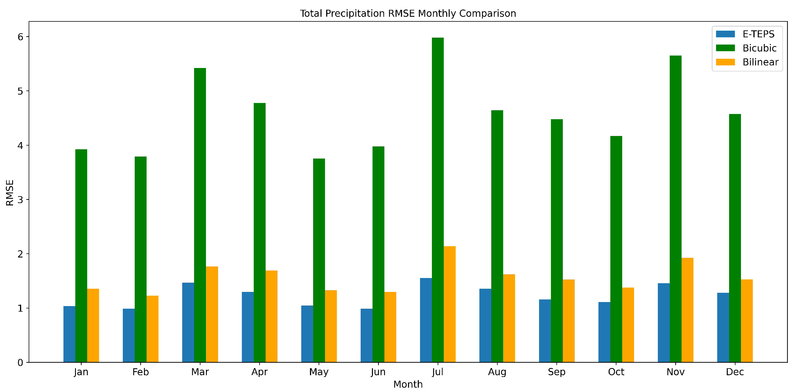
Figure 2 presents the RMSE values for precipitation in each month during 2022. Our model consistently outperforms both bicubic and bilinear interpolation methods across all months, achieving the lowest RMSE values. This superior performance can be attributed to the SRGAN’s ability to learn complex non-linear relationships and generate high-resolution images that closely resemble true high-resolution data. This improvement is especially notable during months with higher precipitation variability, such as April and November.
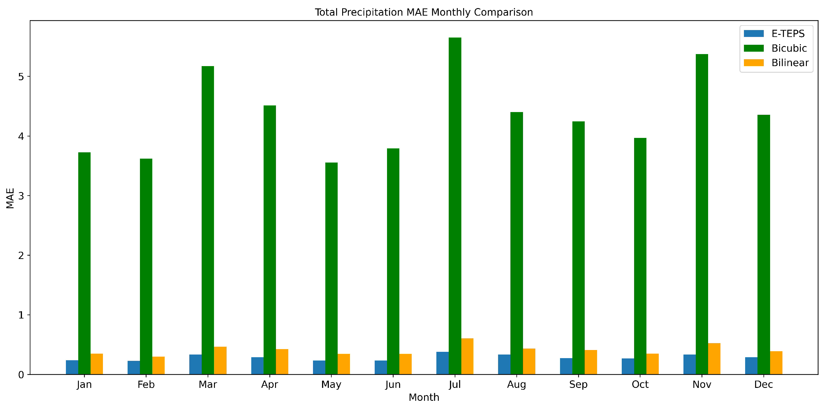
The MAE values for precipitation, shown in
Figure 3, further confirm the advantage of our model. Similar to the RMSE results, E-TEPS exhibits lower MAE values compared to traditional interpolation methods, highlighting its ability to minimize absolute errors in precipitation predictions. This capability is crucial for applications requiring precise rainfall estimates, such as flood forecasting and water resource management [
28]. Lower RMSE and MAE values indicate higher accuracy in predictions, reducing potential errors in flood risk assessment and ensuring more reliable water management decisions [
29].
3.1.2. 2m Temperature
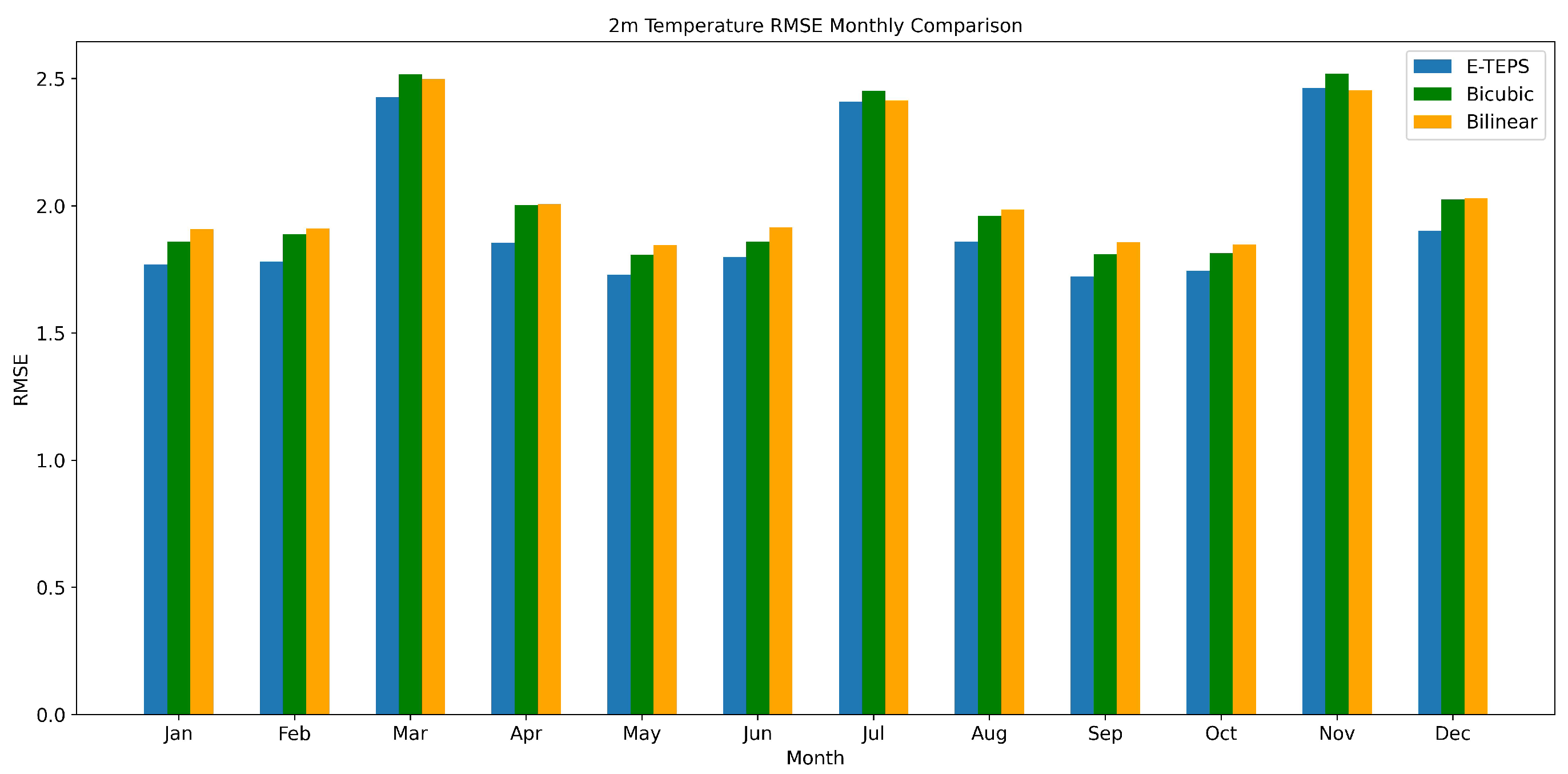
Figure 4 presents the RMSE values for temperature. Although the performance gap between E-TEPS and traditional methods is less pronounced than for precipitation, E-TEPS still demonstrates the lowest RMSE values for most months. This indicates its robustness in temperature downscaling, despite the relatively smaller performance gap.
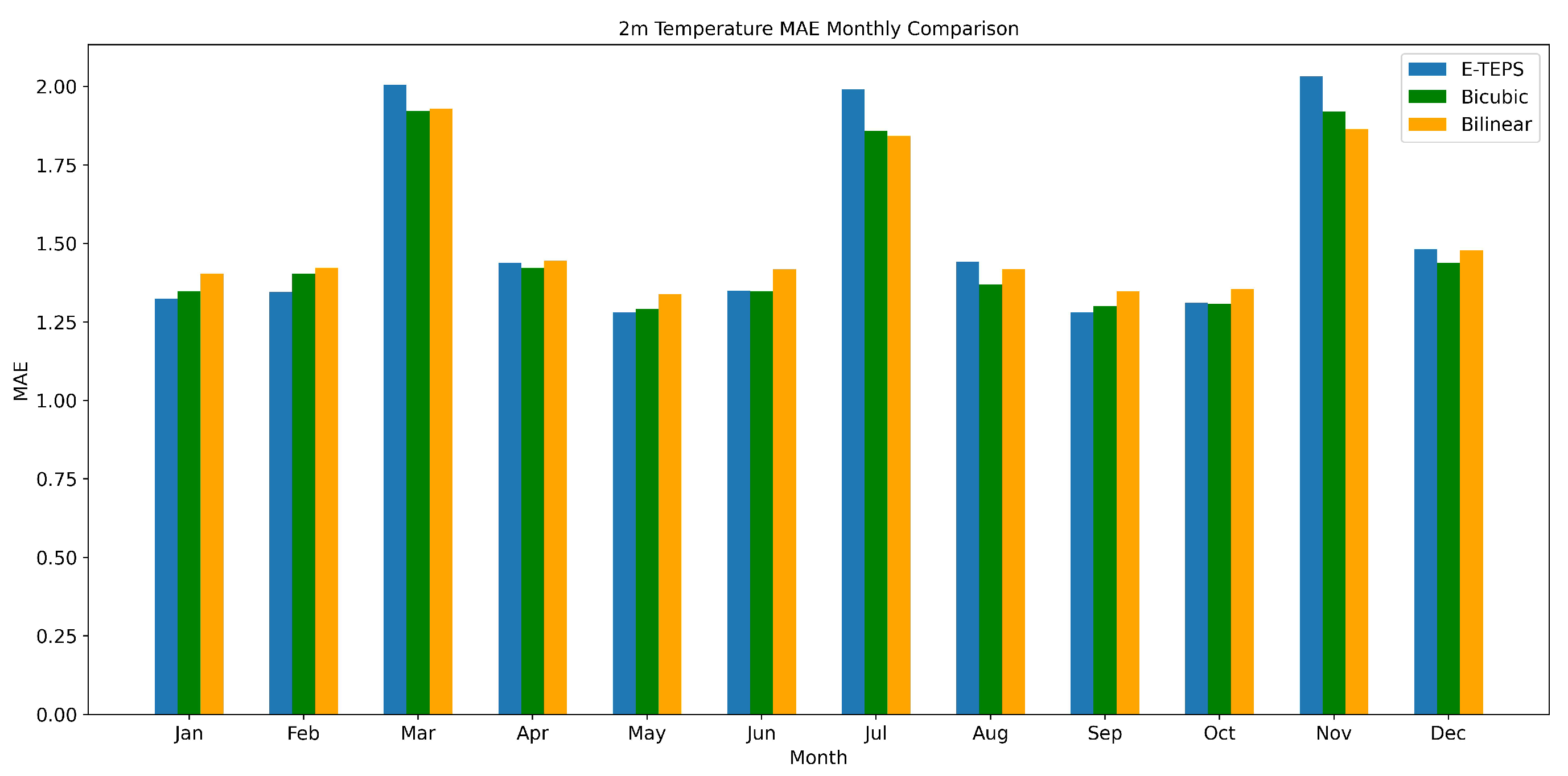
The MAE values for temperature, depicted in
Figure 5, show a similar trend. E-TEPS achieves lower MAE values compared to bicubic and bilinear interpolation across most months.
3.2. Total Precipitation Agreement Analysis
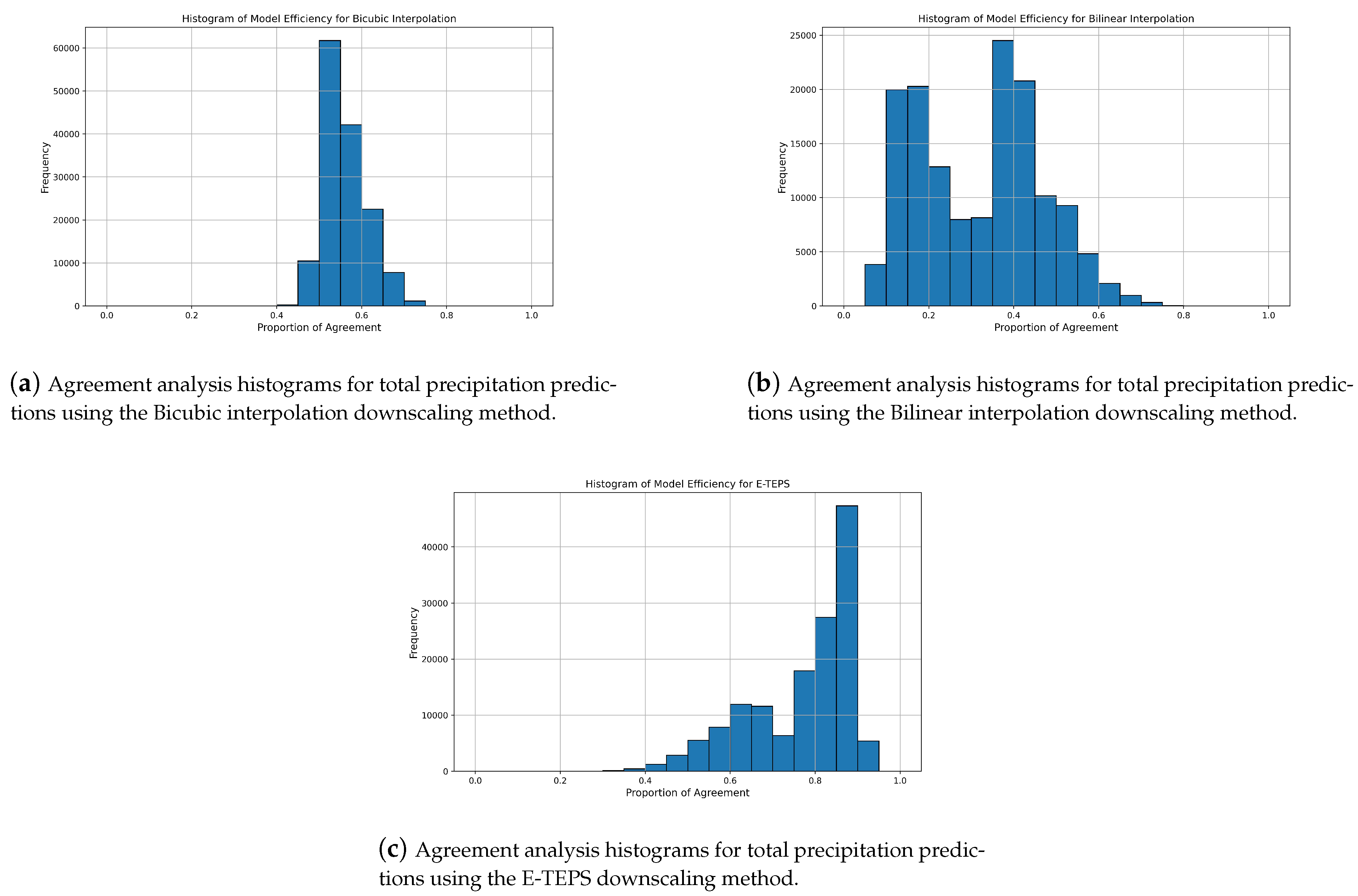
The histogram for Bicubic Interpolation shows a relatively narrow distribution with a peak around 0.5, indicating moderate agreement between the predicted and observed precipitation (
Figure 6a). However, the frequency of high agreement proportions is low, suggesting that Bicubic Interpolation may not consistently capture the finer details of precipitation patterns. In contrast, the histogram for Bilinear Interpolation presents a more dispersed distribution with notable peaks around 0.2 and 0.4, reflecting significant variation in agreement levels and indicating that Bilinear Interpolation struggles to accurately predict precipitation occurrences (
Figure 6b).
The E-TEPS histogram exhibits a much more favorable distribution with a pronounced peak near 0.8, reflecting strong agreement between the downscaled and ground-truth data (
Figure 6c). This high peak indicates that E-TEPS is highly effective in capturing the intricate patterns of precipitation, with a higher frequency of high agreement proportions compared to traditional interpolation methods.
3.3. Pearson Correlation For Temperature
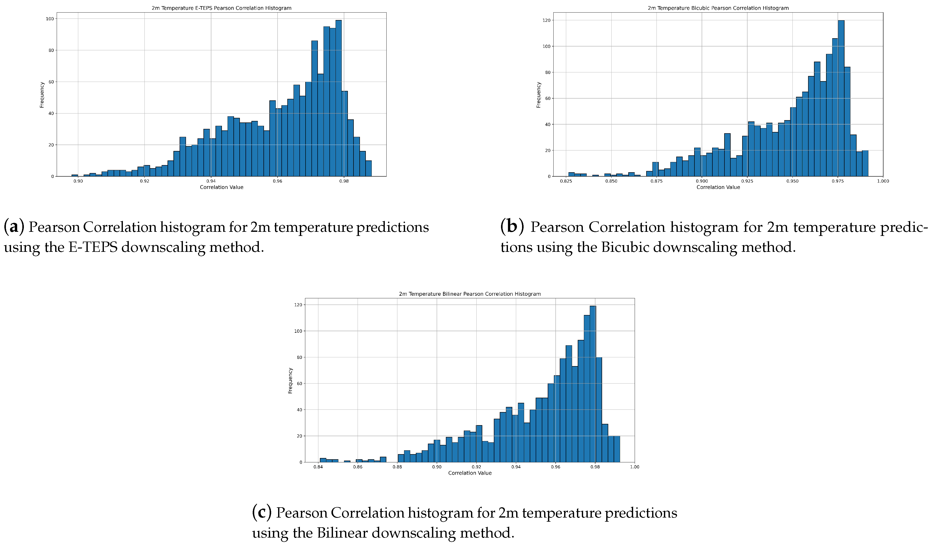
Figure 7 presents the Pearson Correlation histograms for temperature. E-TEPS again demonstrates higher correlation values. The consistent performance of E-TEPS in maintaining high Pearson Correlation values for temperature indicates its effectiveness in preserving spatial patterns [
30].
The histogram for the E-TEPS, shown in
Figure 7a, displays a slightly wider range of correlation values compared to the Bicubic and Bilinear methods. Peaks are observed around 0.96 and 0.98, indicating strong correlation for most predictions, with a range extending from 0.90 to 1.0. This broader distribution reflects the E-TEPS’s ability to capture finer details and more complex patterns in the temperature data, which may result in slight variability. Despite this, the majority of E-TEPS predictions still exhibit high correlation values, highlighting its robustness and potential for delivering superior predictive performance.
In comparison,
Figure 7b and
Figure 7c illustrate that both the Bicubic and Bilinear methods produce somewhat lower correlation predictions. The Bicubic method shows correlation values primarily between 0.825 and 1.0, with a clustering around 0.975. The Bilinear method has correlation values ranging from 0.84 to 1.0, also peaking around 0.975. While these methods are generally reliable and stable, their narrower range and lower peak frequencies indicate a lesser ability to capture complex spatial patterns compared to E-TEPS. The superior performance of our model in maintaining high correlation values across a broader range of conditions underscores its advanced capability in downscaling temperature data with higher fidelity.
3.4. Visual Comparison
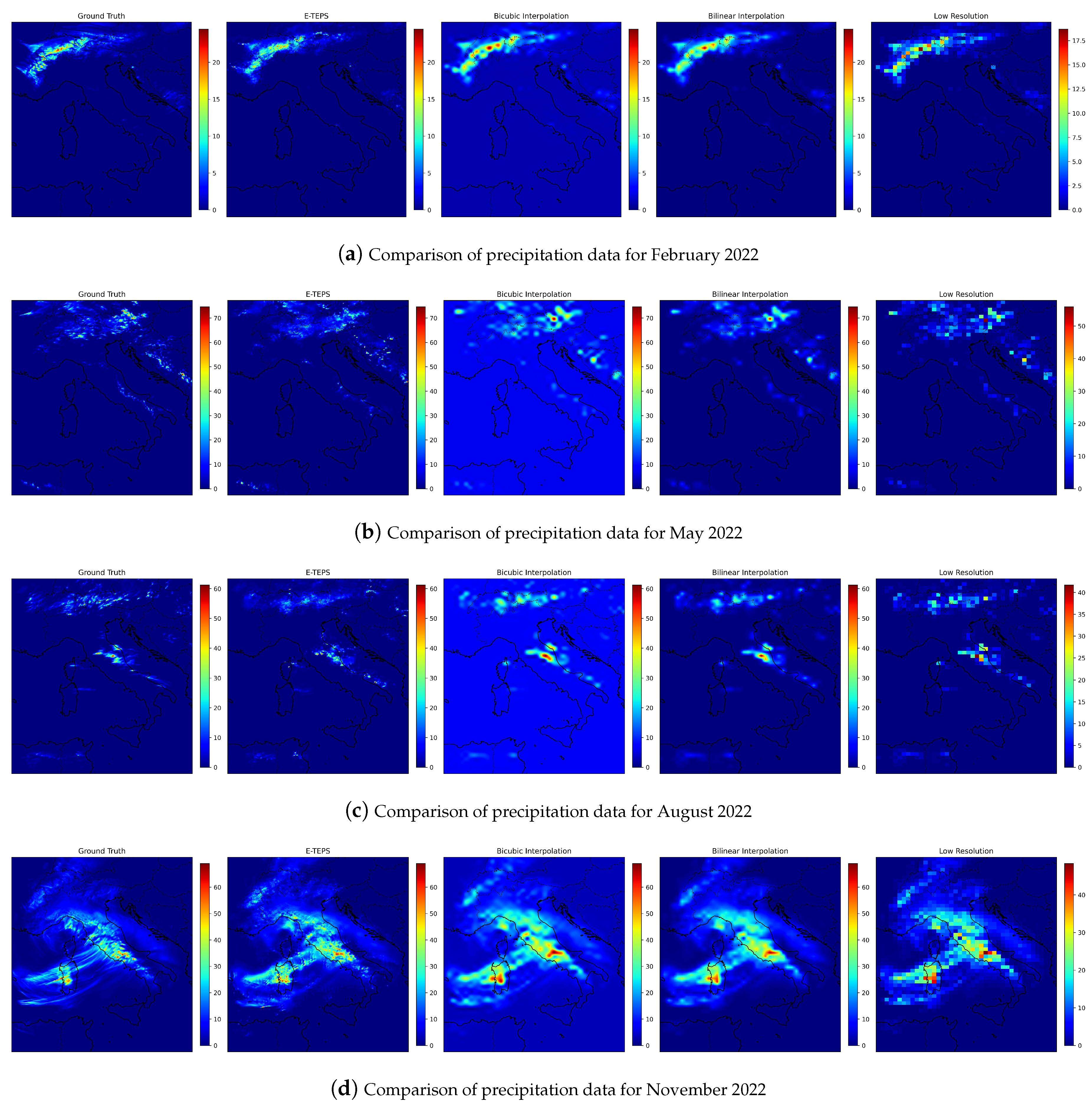
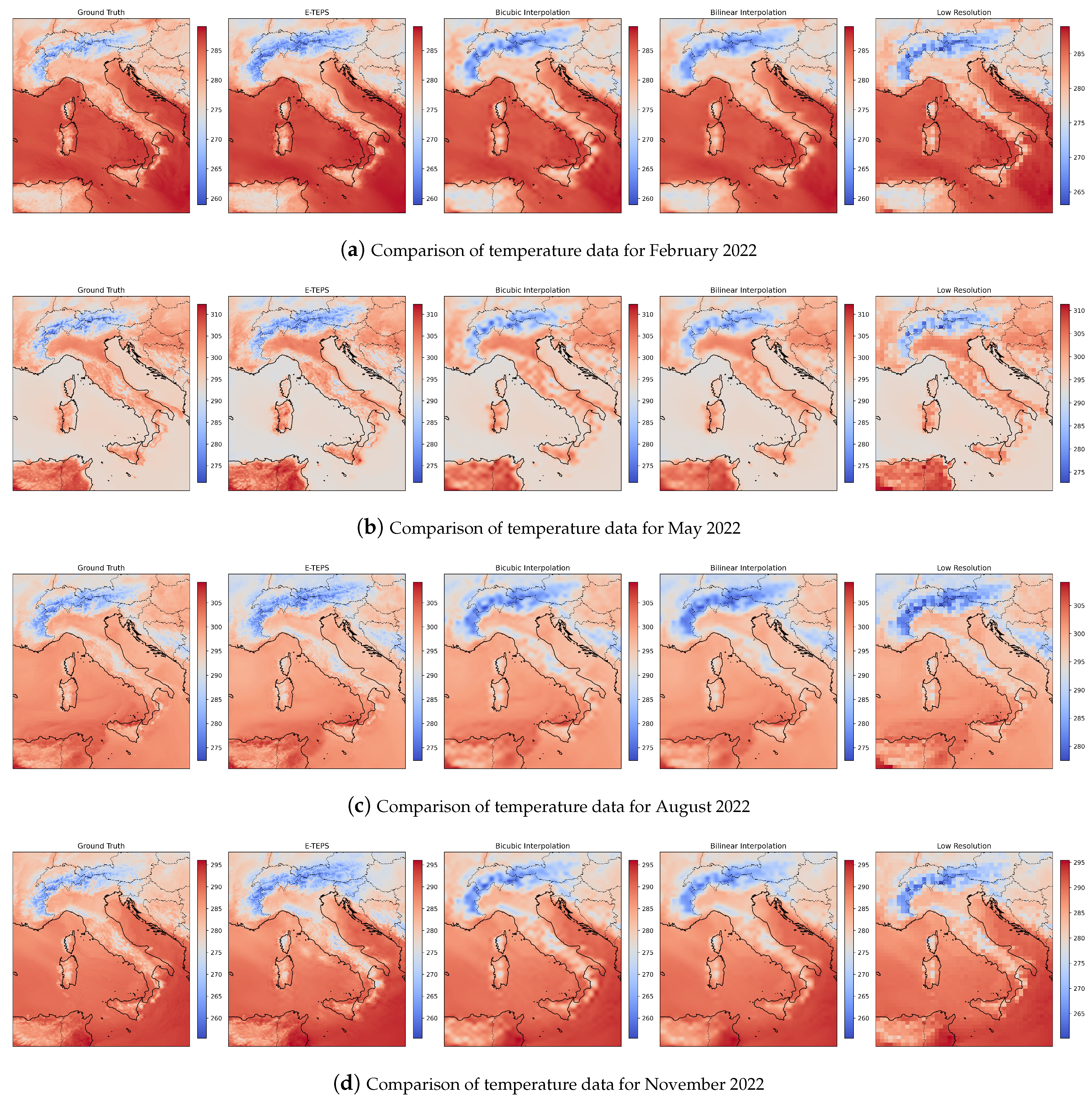
For visual comparison, we selected one timesteps from each season, representing both temperature and precipitation. The selected maps are presented in
Figure 8 and
Figure 9. The visual comparison reveals that E-TEPS generated images closely resemble true high-resolution images, with fewer artifacts and better preservation of fine details. This is particularly noticeable in regions with complex terrain and varying climatic conditions.
For precipitation (
Figure 8), the E-TEPS generated images capture the intensity and distribution of precipitation more accurately than bicubic and bilinear interpolation, evident in the higher-resolution details and fewer artifacts. For temperature (
Figure 9), our model effectively reproduces the temperature patterns observed in true high-resolution images, especially in regions with significant temperature gradients.
Figure 1.
Elevation Map used in Model
Figure 1.
Elevation Map used in Model
Figure 2.
Monthly comparison of the Root Mean Square Error (RMSE) for total precipitation predictions using E-TEPS, Bicubic, and Bilinear downscaling methods.
Figure 2.
Monthly comparison of the Root Mean Square Error (RMSE) for total precipitation predictions using E-TEPS, Bicubic, and Bilinear downscaling methods.
Figure 3.
Monthly comparison of the Mean Absolute Error (MAE) for total precipitation predictions using E-TEPS, Bicubic, and Bilinear downscaling methods.
Figure 3.
Monthly comparison of the Mean Absolute Error (MAE) for total precipitation predictions using E-TEPS, Bicubic, and Bilinear downscaling methods.
Figure 4.
Monthly comparison of the Root Mean Square Error (RMSE) for 2m temperature predictions using E-TEPS, Bicubic, and Bilinear downscaling methods.
Figure 4.
Monthly comparison of the Root Mean Square Error (RMSE) for 2m temperature predictions using E-TEPS, Bicubic, and Bilinear downscaling methods.
Figure 5.
Monthly comparison of the Mean Absolute Error (MAE) for 2m temperature predictions using E-TEPS, Bicubic, and Bilinear downscaling methods.
Figure 5.
Monthly comparison of the Mean Absolute Error (MAE) for 2m temperature predictions using E-TEPS, Bicubic, and Bilinear downscaling methods.
Figure 6.
Agreement analysis histograms for total precipitation predictions using Bicubic, Bilinear, and E-TEPS downscaling methods.
Figure 6.
Agreement analysis histograms for total precipitation predictions using Bicubic, Bilinear, and E-TEPS downscaling methods.
Figure 7.
Pearson Correlation histograms for 2m temperature predictions using Bicubic, Bilinear, and E-TEPS downscaling methods.
Figure 7.
Pearson Correlation histograms for 2m temperature predictions using Bicubic, Bilinear, and E-TEPS downscaling methods.
Figure 8.
Comparative analysis of precipitation data for February, May, August, and November 2022, visualizing Ground Truth, E-TEPS, Low Resolution, Bicubic Interpolation, and Bilinear Interpolation methods. The units are in millimeter.
Figure 8.
Comparative analysis of precipitation data for February, May, August, and November 2022, visualizing Ground Truth, E-TEPS, Low Resolution, Bicubic Interpolation, and Bilinear Interpolation methods. The units are in millimeter.
Figure 9.
Comparative analysis of 2m temperature data for February, May, August, and November 2022, visualizing Ground Truth, E-TEPS, Low Resolution, Bicubic Interpolation, and Bilinear Interpolation methods. Units are in Kelvin.
Figure 9.
Comparative analysis of 2m temperature data for February, May, August, and November 2022, visualizing Ground Truth, E-TEPS, Low Resolution, Bicubic Interpolation, and Bilinear Interpolation methods. Units are in Kelvin.
