
Submitted:
19 August 2024
Posted:
21 August 2024
You are already at the latest version
Abstract
In this paper, we establish the existence and uniqueness results of the fractional Navier-Stokes evolution equation using the Banach fixed point theorem, where the fractional order β is in the form of the Atangana-Baleanu Caputo fractional order. The iterative method combined with the Laplace transform and Sumudu transform are employed to find the exact and approximate solutions of the fractional Navier-Stokes equation of a one-dimensional problem of unsteady flow of a viscous fluid in a tube. Mathematica software is used to present the solutions graphically.
Keywords:
Atangana‐Baleanu Caputo fractional derivative
; Navier‐Stokes equation
; Laplace transform
; Sumudu transform
; iterative method (IM)
1. Introduction
In this paper, we discuss the existence and the uniqueness of the solution of the time- fractional Navier-Stokes equation of a viscous fluid in unsteady flow through a tube applied to Atangana-Baleanu Caputo fractional derivative (fractional derivatives without singular kernel). The Navier-Stokes equation is specified as the nonlinear partial differential equation that describes the motion of an incompressible Newtonian fluid and it was named in honor of French engineer Claude-Louis Navier (1785-1836) and English physicist and mathematician Sir George Gabriel Stokes (1819-1903). Is referred to as Newtonian fluid because it was derived using Newton's second law of motion by considering the forces acting on the fluid elements so that the stress tensor appears in the form of the usual Cauchy momentum equation. This Navier-Stokes equation is the generalization of the equation of motion pioneered by the famous Swiss mathematician Leonhard Euler (1707-1783) to describe the flow of incompressible and frictionless fluids. Navier-Stokes equations are used to model water flow in a pipe, weather forecasting, ocean currents, and airflow around a wing [1]. Furthermore, they assist with the design of cars and aircraft, the study of blood flow, the analysis of pollution, the design of power stations, and a lot of other things. Together with Maxwell's equations, they may be utilized to model and study the magneto-hydrodynamics [1].
The fractional Navier-Stokes equation has been handled by many researchers, such as in [2,3,4,5,6,7,8]. In [7] the Adomian decomposition method (ADM) was utilized by applying the operator , the inverse of the operator on both sides of the fractional Navier-Stokes equation, where is the Caputo time-fractional differential operator of order . The Caputo time fractional Navier-Stokes equation, which describes the motion of a viscous fluid in a tube, has been solved in [4] by combining the Laplace transform with the Adomian decomposition approach. In [2], the Caputo time fractional Navier-Stokes equation describing the motion of a viscous fluid in a tube was solved using the homotopy perturbation transform method (HPTM). In [3], the Caputo-Fabrizio time-fractional Navier-Stokes equation was solved utilizing the iterative Laplace transform method (ILTM). The existence and uniqueness of the Navier-Stokes equation solutions with fractional time derivatives were examined in [5]. The improved Navier-Stokes (N-S) equation with fractional derivative to explore the unsteady translational motion of a rigid sphere in an incompressible viscous fluid was handled in [6].
In [2], the Navier-Stokes equation is determined as the essential condition of computational liquid elements, relating pressure and external forces following up on a liquid to the reaction of the liquid stream.
In this study, we model the fractional Navier-Stokes equation. The fractional Navier-Stokes and continuity equation are given as
where, is the fluid velocity, is the fluid pressure, is the fluid viscosity, is the fluid density, is the Caputo fractional derivative, is the gradient differential operator and is the Laplacian operator. It is important to mention that, if the viscosity is set equal to zero, then the Navier-Stokes equation (1) reduces to Euler's equation of motion of incompressible and frictionless fluids.
Because our objective is to access the impact of the Mittag-Leffler kernel on the Navier-Stokes system, hence, we replace with in Eq. (1), so that the resulting equation is the fractional Navier-Stokes equation in Atangana-Baleanu Caputo sense. Therefore, we consider the new fractional Navier-Stokes equation in the Atangana-Baleanu Caputo sense and its initial condition as
Then we intend to find the solution using the Laplace or Sumudu transform of the ABCFD coupled with the iterative method (IM) applied to a one-dimensional problem of unsteady flow of a viscous fluid in a tube. The advantage of using this method is that we combine the two methods, namely: the Laplace or Sumudu transform and the iterative method (IM) which are very useful for finding the exact and approximate solutions of linear and nonlinear differential equations, moreover the method helps with avoiding many and complicated computational tasks as compared to the normal technique. Another advantage is that the ABCFD applied in Equation (2) is non-local, meaning that when modeling a real physical phenomenon, the state of the system does not only depend on the present time but also the history.
The fractional Navier-stokes equation (2) along with its initial condition can be written in terms of cylindrical coordinates as follows (see
subject to the following initial condition
where is the Atangana-Baleanu fractional derivative in Caputo sense.
2. Preliminaries
In this section, we recall some definitions and theorems of fractional calculus which are very important for our study.
Definition 2.1. Let , then Atangana-Baleanu Fractional Derivative in Caputo sense is given by
where is a normalization function such that and is the Mittag-Leffler function (MLF) defined as:
Theorem 2.1. The Laplace transform of the ABCFD is specified as
Definition 2.3. The Sumudu transform of the ABCFD is defined as follows [11]:
Theorem 2.2. The ABCFD and its fractional integral of a function satisfy the Newton-Leibniz formula
where is the Atangana-Baleanu fractional integral so that we have
3. Existence and Uniqueness of Nonlinear Fractional Derivatives with Respect to ABCFD
In this section, we apply Banach fixed-point theorem to establish the existence and uniqueness results of the fractional initial value problem and we further show that the results also hold for fractional Navier-Stokes equation (3) and the initial condition (4).
To continue we consider the following fractional initial value problem
Theorem 3.1. Let , then is a solution to the fractional initial value problem (10), if and only if, it is a solution to the following integral equation
Proof of Theorem 3.1. Applying the Atangana-Baleanu fractional integral on both sides of Equation (10) and utilizing the properties of the inverse operator, will lead us to Equation (11). □
Theorem 3.2. Consider the fractional initial value problem (10), where is a smooth function. If is the Lipschitz function with Lipschitz constant
then the fractional initial value problem (10) has a unique solution in .
Proof of Theorem 3.2. Define the norm on by
and consider the operator , defined by
According to Theorem 3.1, obtaining a solution to the initial value problem (10) is equivalent to finding a fixed point of . Now, for all and , we have
Since , therefore is contraction and according to Banach fixed point theorem, has a unique fixed point.
□
Now we apply theorem 3.1 and theorem 3.2 to fractional Navier-stokes equation (3). If we replace of equation (10) with of the fractional Navier-stokes equation (3) and also the initial condition replaced with , then according to theorem 3.1 and 3.2 the fractional Navier-stokes equation (3) with its initial condition has a unique solution in .
Remark 3.1. [13] For , and , we have
Thus, if is Lipschitz function with Lipschitz constant , therefore the fractional initial value problem (10) has a unique solution in , for all .
4. Analysis of the Fractional Navier-Stokes Equation with ABCFD
In this section, we consider the Navier-Stokes equation for the one-dimensional motion of a viscous fluid in a tube with an unsteady flow. We solve the fractional Navier-stokes equation applied to the ABCFD using the iterative Laplace transform method (ILTM).
Consider the following Navier-stokes equation in cylindrical coordinates
subject to the following initial condition
If we apply the fractional derivative of order in Equation (13) at the extant time derivative term, we obtain:
We can write Equation (15) in terms of the Atangana-Baleanu fractional derivative in the Caputo sense as follows:
where
Applying the Laplace transform (7) on both sides of Equation (16) and use the initial condition (14), we get
Applying the inverse Laplace transform on both sides of Equation (19), we get
where .
The term represents the term arising from the source term and the given initial conditions. Then if we apply the iterative method, we obtain the solution as an infinite series:
substituting (21) in (20), we obtain:
Comparing the coefficients of , we get:
Thus, series solution of (16)
4.1. Numerical Examples
We provide some numerical examples to demonstrate the proficiency and correctness of our solution of the Atangana-Baleanu fractional Navier-Stokes equation in Caputo sense utilizing the iterative Laplace transform method (ILTM) and iterative Sumudu transform method (ISTM).
Example 4.1. The time-fractional Navier-Stokes equation concerning the ABCFD with is given as:
subject to the following initial condition
Applying the Laplace transform (7) on both sides of Equation (29) and using the above initial condition we obtain:
Applying the Laplace inverse on both sides of Equation (30), we get
where
Applying the iterative method coupled with the Laplace transform, we obtain:
Comparing the coefficients of , we get:
so that
for all .
The series solution of Equation (29) is as follows:
and we see that with only the third order term, we obtain the exact solution, and if we let we obtain the classical solution of the normal Navier-Stokes equation as
Figure 1 illustrates the graphical representation for the solution of Equation (29), for when (a) , (b) , (c) and (d) .
Figure 2 illustrates the graphical representation for the solution of Equation (29), for and when and .
Figure 3 illustrates the graphical representation for the solution of Equation (29), for and when and .
From the numerical results illustrated in Figure 1, Figure 2 and Figure 3, is simple to conclude that the solution is continuously dependent on the time-fractional derivative.
Example 4.2. Now we illustrate how to find the solution of Equation (29): (Example 4.1) subject to the same initial condition: via the iterative Sumudu transform method (ISTM).
Applying the Sumudu transform (8) on both sides of Equation (29) and using its initial condition, we obtain:
where is the Sumudu transform.
Applying the Sumudu inverse on both sides of Equation (37), we get
where
Applying the iterative method coupled with the Sumudu transform, we obtain:
Comparing the coefficients of , we get:
so that
for all .
The series solution of Equation (29) is as:
Then if we obtain the same classical solution of example 4.1.
Example 4.3. Consider the following time-fractional Navier-Stokes equation with respect to the ABCFD
subject to the following initial condition
Applying the Laplace transform (7) on both sides of Equation (43) and using the above initial condition we obtain:
Applying the Laplace inverse on both sides of Equation (44), we get
where
Applying the iterative method combined with the Laplace transform, we obtain:
Comparing the coefficients of , we get:
so that
The series solution of Equation (43) is as:
If we use the gamma function property , then we can write (48) as
The approximate solution for Equation (43), when is given by and the graphical representation is provided in Figure 4.
Figure 4 illustrates the graphical representation for the solution of Equation (43), when and (a) , (b) , (c) and (d) .
Remark 4.1. If we consider the Navier Stokes equation in example 4.1 with the viscosity , then the fractional Navier Stokes equation (29) will reduce to the Euler's equation of the incompressible and frictionless fluid of the form
subject to the initial condition
so that according to example 4.1 and 4.2, is the exact solution of the Euler's equation, if .
6. Conclusions
In this paper, the iterative method was utilized to solve time-fractional Navier-Stokes equations applied to a one-dimensional problem of unsteady flow of a viscous fluid in a tube along with the initial conditions. The fractional derivative was specified in terms of the Atangana-Baleanu Caputo sense. The method was coupled with the Laplace and Sumudu transform to assist with getting the exact and approximate solutions. The analytical results have been provided in terms of a power series with simple computable terms and it is observed that the solution found by this method rapidly converges to the exact solution. The results demonstrate that the solution continuously depends on the time-fractional derivative. We also provided the graphical representation of the solutions using Mathematica software. Finally, the iterative method coupled with the Laplace or Sumudu is a very powerful and efficient technique to be used to obtain analytical solutions for various types of fractional linear, nonlinear and partial differential equations and we hope that our work is heading in the right direction in term of solving the problems involving such equations.
Funding
This research received no external funding.
Informed Consent Statement
Not applicable.
Data Availability Statement
Data sharing is not applicable to this article
Conflicts of Interest
The authors declare no conflicts of interest.
Abbreviations
The following abbreviations are used in this manuscript:
ABCDF Atangana-Baleanu Caputo fractional. Derivatives
ABFI Atangana-Baleanu fractional integral.
IM Iterative method.
MLF Mittag-Leffler function.
N-S Navier-Stockes.
References
- Akbar, T.; Zia, Q.M.Z. Some Exact Solutions of Two-Dimensional Navier–Stokes Equations by Generalizing the Local Vorticity. Advances in Mechanical Engineering 2019, 11, 168781401983189. [Google Scholar] [CrossRef]
- Kumar, D.; Singh, J.; Kumar, S. A Fractional Model of Navier–Stokes Equation Arising in Unsteady Flow of a Viscous Fluid. Journal of the Association of Arab Universities for Basic and Applied Sciences 2015, 17, 14–19. [Google Scholar] [CrossRef]
- Yadav, L.K.; Agarwal, G.; Kumari, M. Study of Navier-Stokes Equation by Using Iterative Laplace Transform Method (ILTM) Involving Caputo- Fabrizio Fractional Operator. J. Phys.: Conf. Ser. 2020, 1706, 012044. [CrossRef]
- Kumar, S.; Kumar, D.; Abbasbandy, S.; Rashidi, M.M. Analytical Solution of Fractional Navier–Stokes Equation by Using Modified Laplace Decomposition Method. Ain Shams Engineering Journal 2014, 5, 569–574. [Google Scholar] [CrossRef]
- Zhou, Y.; Peng, L. On the Time-Fractional Navier–Stokes Equations. Computers & Mathematics with Applications 2017, 73, 874–891. [Google Scholar] [CrossRef]
- Ashmawy, E.A. Unsteady Translational Motion of a Slip Sphere in a Viscous Fluid Using the Fractional Navier-Stokes Equation. Eur. Phys. J. Plus 2017, 132, 142. [Google Scholar] [CrossRef]
- Momani, S.; Odibat, Z. Analytical Solution of a Time-Fractional Navier–Stokes Equation by Adomian Decomposition Method. Applied Mathematics and Computation 2006, 177, 488–494. [Google Scholar] [CrossRef]
- Biazar, J.; Babolian, E.; Kember, G.; Nouri, A.; Islam, R. An Alternate Algorithm for Computing Adomian Polynomials in Special Cases. Applied Mathematics and Computation 2003, 138, 523–529. [Google Scholar] [CrossRef]
- Atangana, A.; Baleanu, D. New Fractional Derivatives with Nonlocal and Non-Singular Kernel: Theory and Application to Heat Transfer Model. Therm sci 2016, 20, 763–769. [Google Scholar] [CrossRef]
- Atangana, A.; Owolabi, K.M. New Numerical Approach for Fractional Differential Equations. Math. Model. Nat. Phenom. 2018, 13, 3. [Google Scholar] [CrossRef]
- Bokhari, A.; Baleanu, D.; Belgacem, R. Application of Shehu Transform to Atangana-Baleanu Derivatives. J. Math. Computer Sci. 2019, 20, 20–107. [Google Scholar] [CrossRef]
- Alomari, A.K. Homotopy-Sumudu Transforms for Solving System of Fractional Partial Differential Equations. Adv Differ Equ 2020, 2020, 222. [Google Scholar] [CrossRef]
- Syam, M.I.; Al-Refai, M. Fractional Differential Equations with Atangana–Baleanu Fractional Derivative: Analysis and Applications. Chaos, Solitons & Fractals: X 2019, 2, 100013. [Google Scholar] [CrossRef]
Figure 1.
Exact solution of Equation (29) with the initial condition for and 1.
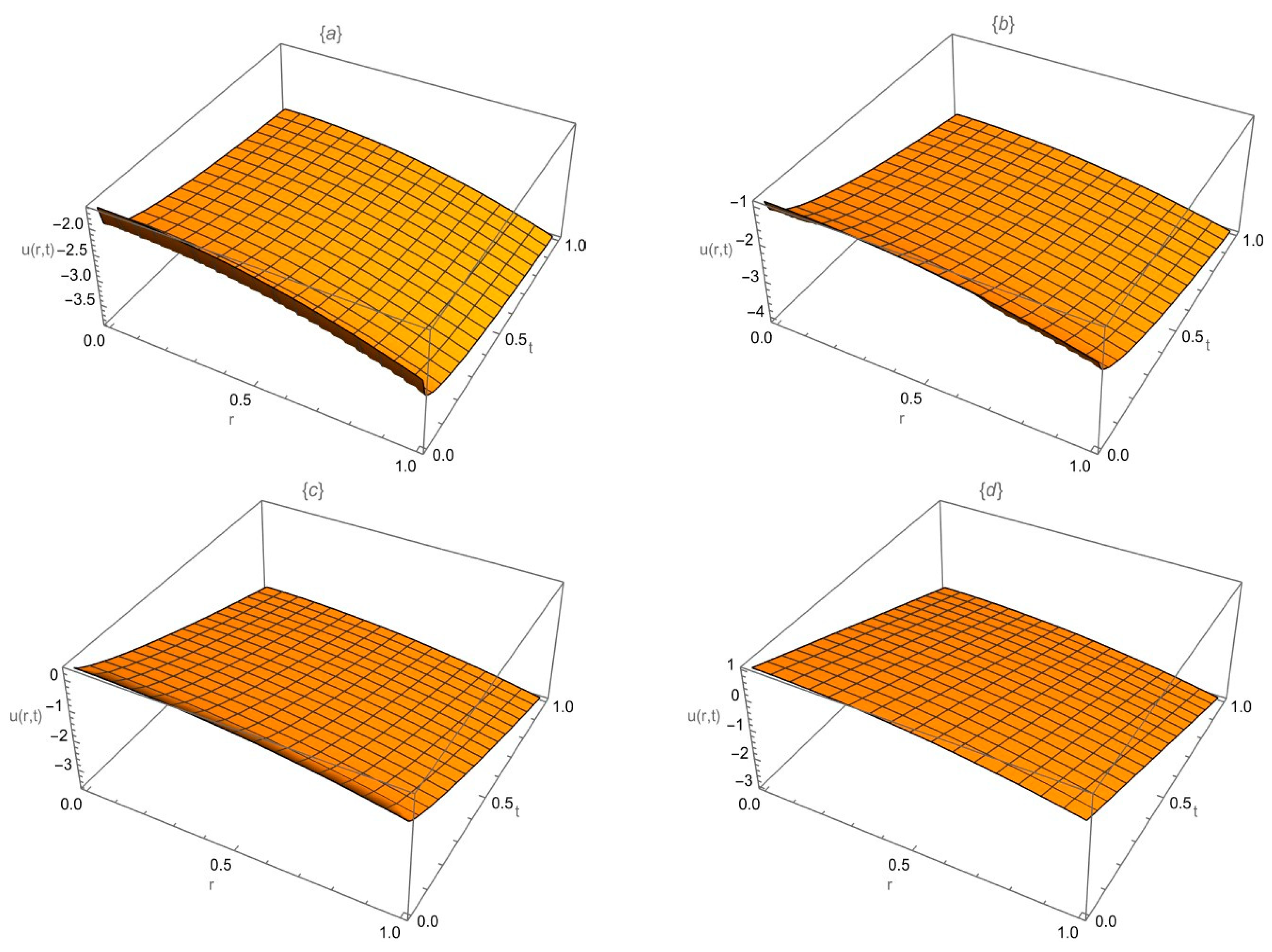
Figure 2.
Solution of Equation (29) when for and 1.
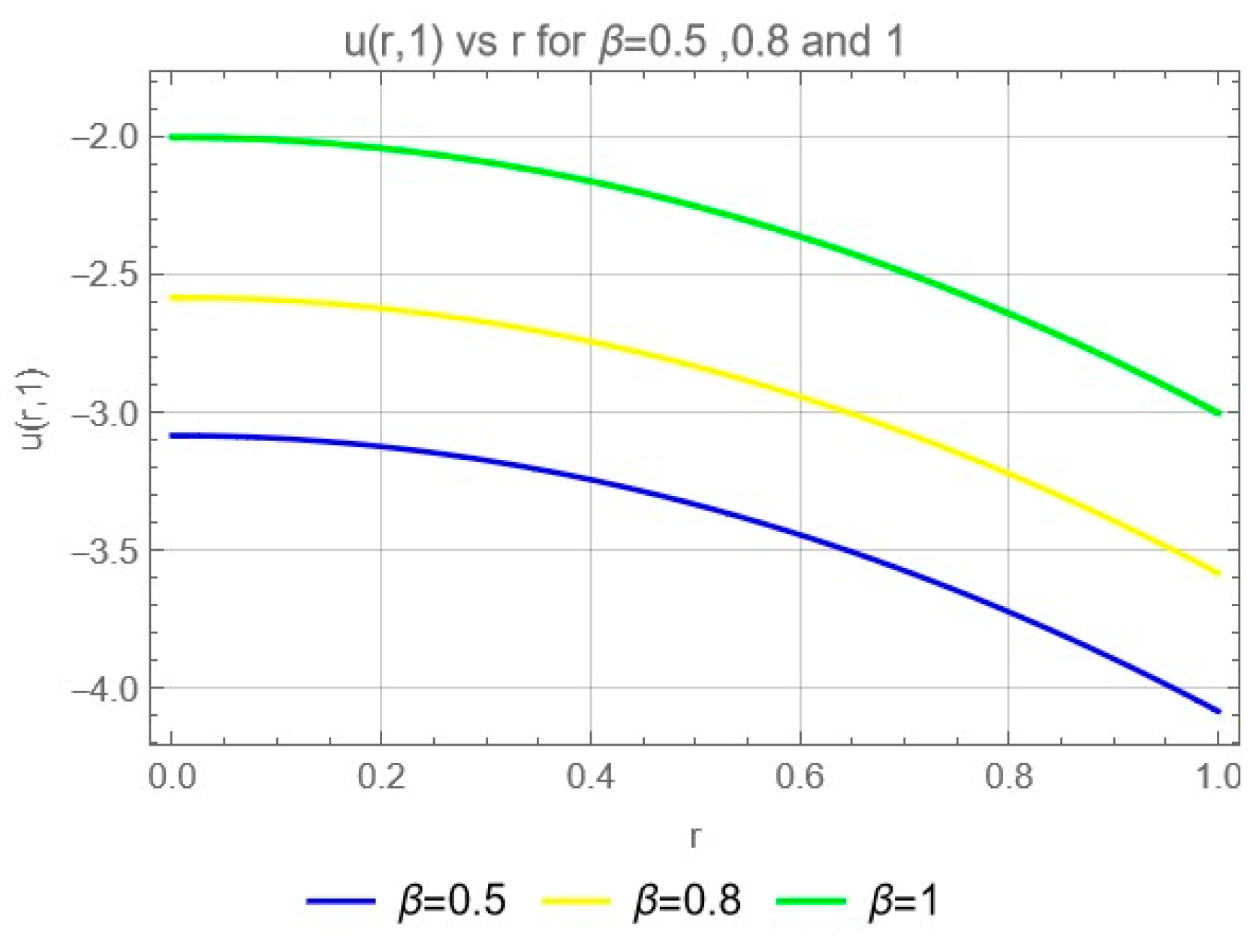
Figure 3.
Solution of Equation (29) when for and 1.
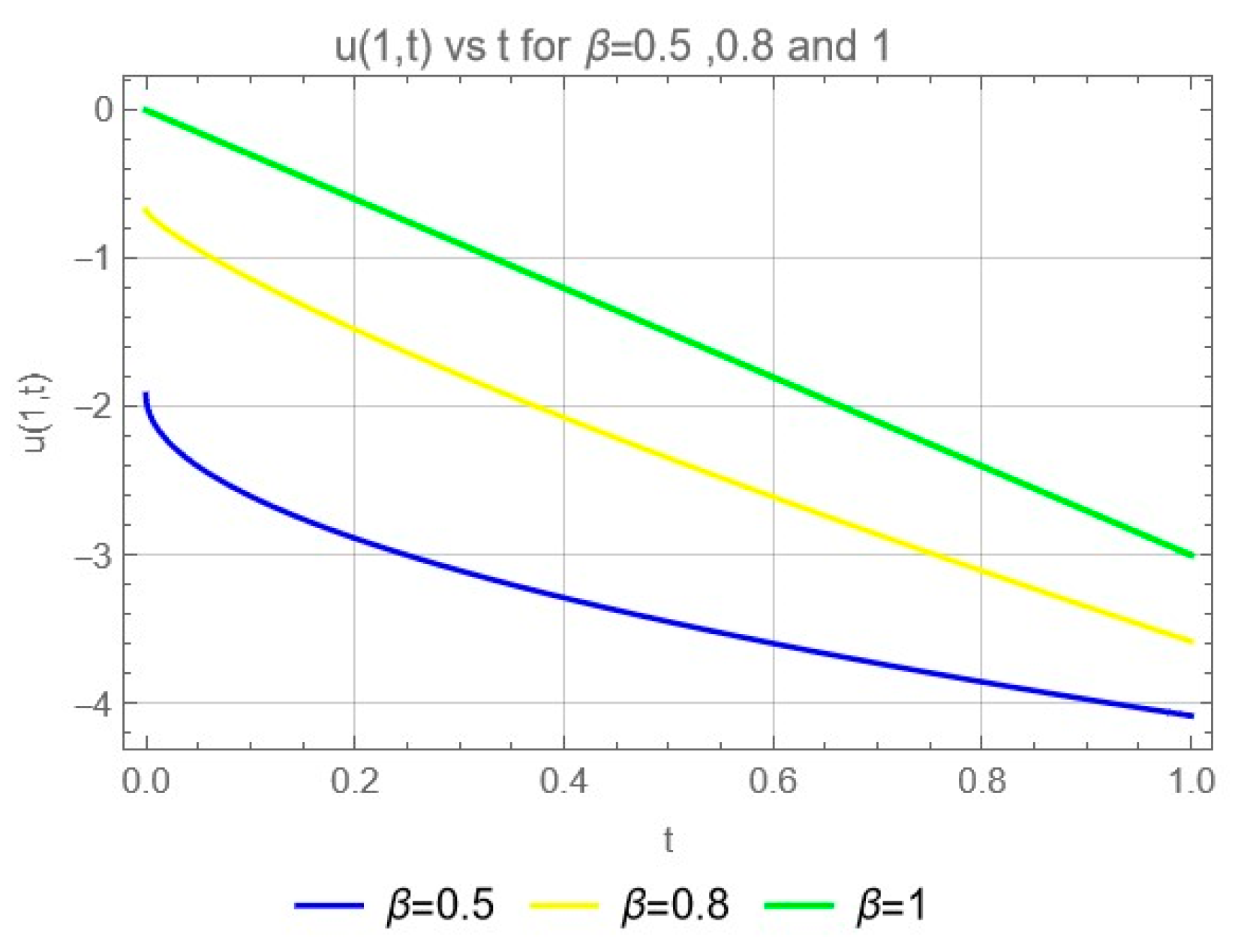
Figure 4.
Approximate solution of Equation (43) with the initial condition for and 1.
Disclaimer/Publisher’s Note: The statements, opinions and data contained in all publications are solely those of the individual author(s) and contributor(s) and not of MDPI and/or the editor(s). MDPI and/or the editor(s) disclaim responsibility for any injury to people or property resulting from any ideas, methods, instructions or products referred to in the content. |
© 2024 by the authors. Licensee MDPI, Basel, Switzerland. This article is an open access article distributed under the terms and conditions of the Creative Commons Attribution (CC BY) license (http://creativecommons.org/licenses/by/4.0/).
Copyright: This open access article is published under a Creative Commons CC BY 4.0 license, which permit the free download, distribution, and reuse, provided that the author and preprint are cited in any reuse.


