1. Introduction
The application of 3D scanning technology in product design, development, production, and quality control has not only shortened the overall product development cycle, but due to the nature of the technology, it is rapidly spreading across various fields such as civil engineering, architecture, cultural heritage preservation, healthcare, and computer graphics, garnering attention from diverse sectors. With the rapid advancement of this technology, traditional 2D drawing in design is evolving into production technology where virtual 3D data created on a PC is utilized for manufacturing [
1,
2,
3].
In line with this development, some industries have recently reversed (reversed engineering) this sequential approach, requiring virtual 3D data from actual products. For instance, when a part used in expensive machinery becomes worn out or damaged and needs replacement, if that part is no longer manufactured or lacks CAD data, the expensive machinery could become useless due to this single part. To reproduce this part, the first step is to create CAD data from the physical object. By the spreading 3D scanning solutions, one of the main application areas of 3D scanning technology is reverse engineering [
4].
Reverse engineering (RE) refers to the technology and process of capturing digital shape information from physical objects that lack CAD data using various methods and then generating CAD data based on this. In the past, vernier calipers and other contact measuring devices were used to capture the dimensions of physical shapes, followed by product design work using conventional CAD modeling programs. Alternatively, coordinate measuring machines (CMMs) were used to capture feature points from objects for design purposes [
5,
6]. However, the downside of these methods is the low reliability of the results, as they only capture coordinate values at specific points designated by the user. In other words, after measuring minimal and approximate information sufficient to define a low level of geometric shapes, lengthy CAD modeling work is performed based on this. In contrast, using a 3D scanner allows for the acquisition of high-density measurement data of the target product, enabling the representation of geometric shapes and various freeform surfaces. This can significantly reduce working time and make it easier to design complex surfaces that were difficult to model in the past [
7,
8,
9]. This process is very important as it improves productivity.
With the recent adoption of 3D RE methods, software capable of generating parametric CAD models from 3D scan data has emerged. Unlike past methods that focused on generating NURBS surfaces [
10,
11], this approach automatically extracts the original design intent and process from the 3D scan data, allowing users to trace back the original modeling process. The most critical step in this RE process is performing preprocessing on the point data obtained from the 3D scanner, followed by segmentation and classification before proceeding to surface fitting.
If this step is unclear, much user effort is required for the final CAD model generation stage. If the goal of digitizing a physical product is merely to copy the geometric shape, and the ability to modify the designed model is not important, then a surface model like NURBS (Non-Uniform Rational B-Splines) curve created from point data obtained by the 3D scanner may nearly suffice. However, the practical usefulness of the model obtained after completing the RE process varies depending on several factors, with the most important being the ability to recover the essential design intent that defines the part.
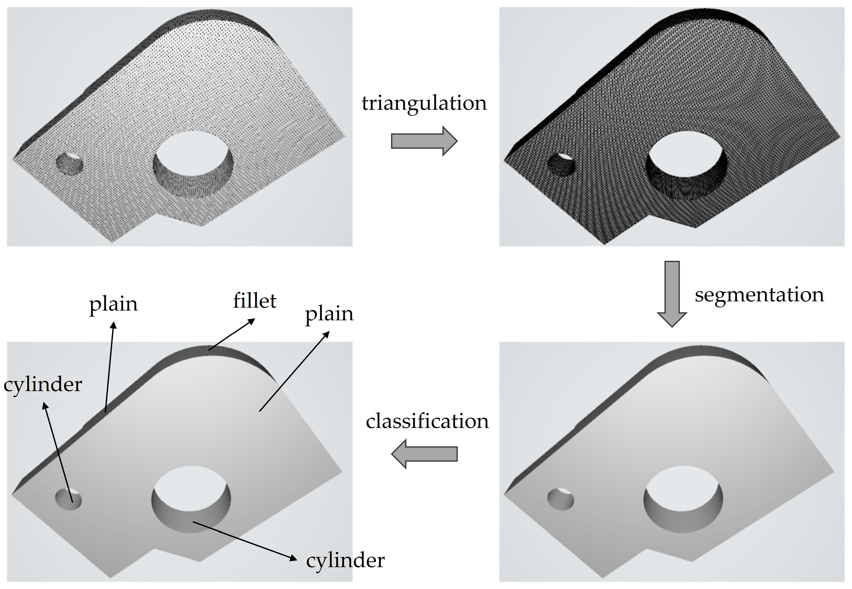
Simply achieving close-representation is not sufficient for engineers, as models need to be defined with precise dimensions and a correct set of geometric relationships and features. Therefore, considering engineering applications, the primary goal of the RE process is to extract information from the acquired raw data and reconstruct an appropriate parametric CAD model that closely matches the object's original design. The CAD functions constructed must be accurate, especially regarding dimensions, assembly structures, and the existing relationships between them as shown in
Figure 1. Through this process, users can redesign the desired shape at a faster speed.
Previous studies have proposed methods that pursue more meaningful reconstructions by introducing a set of geometric constraints during the surface fitting phase defined among identified geometric features. By formulating a constrained optimization problem [
12,
13], satisfactory results can be obtained, but achieving a suitable set of constraints using automated recognition algorithms or relying on user input requires considerable effort. Defining a solvable, non-contradictory, and convenient set of constraints is a crucial task that significantly affects the efficiency of the method. Additionally, in most constraint-fitting formulations, constraints are only implemented up to a specific tolerance [
14]. The accompanying reconstruction errors are typically dimensionally negligible for practical purposes, but these inaccuracies may be inconvenient during subsequent editing.
Another approach involved fitting surfaces independently to build a model in one try [
15]. However, despite the advantage of significantly reducing the mathematical complexity of the procedure by ignoring the original 3D data, this method has the drawback of limited efficiency. Other methods have proposed template-based reconstruction methods, where a sort of CAD template containing known features and geometric relationships is defined at the start of the RE process to guide the reconstruction [
16]. Another method applied known geometric constraints to predefined topologies (e.g., cylindrical slot parts, rectangular slot parts) using a machine learning [
17]. Applying existing techniques can yield satisfactory results when dealing with noisy data that is difficult to analyze, but the reconstructed models are still distinguished by loosely imposed constraints and tolerances that control the rigidity of the constraints. In addition, a probabilistic approach focused on reconstructing cylindrical components for engineering applications has been proposed [
18,
19], and the user’s knowledge is utilized to ensure the consistency of the reconstructed model.
The above-mentioned approaches have two major limitations. The first is the difficulty in fully applying precise geometric constraints while respecting the user's intent and maintaining the model's editability through a well-defined feature tree in an editable parametric CAD model. The second limitation is that most methods assume that the surface is smooth after the preprocessing of point data obtained from the 3D scanner. Smoothing a 3D scan can significantly enhance the quality of your model by removing noise and imperfections. However, the extent amount of smoothing is often determined by the user's intuition. In some cases, excessive smoothing can blur important details, while insufficient smoothing can yield results that deviate from reality. For instance, if a surface that is supposed to be simple and flat still contains a lot of noise after the smoothing process, it might be incorrectly considered a complex shape made up of multiple primitives instead of a single plane. This would require the user to perform an additional step of manually simplifying the complex shape into a plane. Moreover, in cases where the shape is complex, the user might not find the parts, and the complex mesh structure could be carried over into subsequent procedure work.
In this paper, I propose a method for effectively performing classification from 3D point data using environment mapping (EM) and supervised learning (SL) techniques. EM is a technique used in 3D computer graphics to simulate the way surfaces reflect their surrounding environment. This method involves capturing the surrounding environment and mapping it onto the surface of a 3D object to create realistic reflections. After preprocessing the point data, the information is mapped to the environment using the EM technique, and then trained using SL. When new 3D mesh data is given, the EM is performed, and classification is conducted using the data mapped to the environment. Using this method has the advantage of allowing classification at easy even if there are some noises or other wounds on the surface.
The structure of the paper is as follows. In Chapter 2, we present the proposed method and the algorithm that controls the entire process. Chapter 3 discusses the results obtained through a series of test cases. Finally, in the conclusion of Chapter 4, I summarize the proposed method, discuss its strengths and weaknesses, and suggest a future improvement.
2. Methods
2.1. Overview
RE involves a detailed process of deconstructing a product or system to understand its components, structure, and operation as shown in
Figure 2.
The first step is object acquisition, where a physical object is scanned using 3D scanners such as laser, structured light, or CT scanning to capture its geometry. The resulting data is in the form of a point cloud, a collection of data points representing the object’s surface. Following acquisition, the preprocessing stage begins. This involves reducing noise in the raw point cloud data through smoothing, filtering, or outlier removal to enhance data quality. If multiple scans are taken from different angles, they need to be aligned or registered into a single coordinate system. After this, the point cloud is converted into a mesh structure, consisting of vertices, edges, and faces representing the surface geometry. Next is the feature extraction phase, which starts with segmentation, dividing the mesh into different regions based on geometric features like flat surfaces, curves, or edges. These segmented regions are then classified into different categories or types of features, such as flat surfaces, cylindrical shapes, or complex curves. Classification helps determine the appropriate geometric modeling approach for each segment. Following classification, surface fitting is conducted to match geometric features like planes, cylinders, or freeform surfaces onto the classified mesh regions. Model reconstruction is the next step, where the fitted surfaces are used to create a continuous surface model of the object. This surface model is then converted into a solid CAD model, incorporating detailed features such as holes, fillets, and chamfers. Parametric modeling is also performed, where the CAD models are made adjustable through parameters and constraints, allowing modifications to the design. The final step is verification. The stage follows, where the reconstructed model is validated by comparing it against the original scanned data to ensure accuracy. Any discrepancies found are corrected. Additionally, structural, thermal, or dynamic analysis may be performed to ensure the model meets required specifications.
The most critical step in this process is the feature extraction stage. This stage is highly dependent on the outcomes of the previous step, the pre-processing. Even when applying the same algorithm, the results can vary significantly depending on the quality of the pre-processing. Another reason why the feature extraction stage is crucial is that it can significantly reduce the amount of effort required from the user in the subsequent reconstruction and validation steps. The results of feature extraction can differ widely depending on the quality of preprocessing, even when the same methods are used. Therefore, there is a need for a feature extraction method that is less dependent on the preprocessing stage. In this paper, we propose a method that utilizes EM, commonly used in computer graphics, along with SL to address this issue.
There have been previous attempts to apply EM and machine learning together. The paper [
20,
21] proposes a method using GANs (Generative Adversarial Networks) to train models on virtual environment maps, enabling the model to be applied in real-world environments, and the paper [
17,
22,
23] explores combining EM with neural networks to more accurately learn and reproduce the reflective properties of objects. Here, machine learning is used to model the 3D shape and reflective characteristics of objects. That is, these approaches use the EM and machine learning as a crucial tool in the analysis and utilization of 3D data.
2.2. Evvironment Mapping
EM is a technique widely used in computer graphics to create realistic reflections and lighting effects on 3D objects. This technique simulates how a surface reflects its surrounding environment, allowing objects to appear as though they are embedded within a realistic scene. It is particularly useful for simulating reflective surfaces like water, glass, or metal, where capturing the interaction between the object and its environment is crucial for achieving visual realism.
The fundamental concept behind EM is to map the environment around an object onto the surface of the object itself. This mapping creates the illusion that the object is reflecting the environment, even though no actual reflection calculations are being performed. The environment is typically represented as a texture map that is wrapped around the object.
There are several types of EM techniques, including sphere mapping, cube mapping, and parallax mapping, each offering different trade-offs between accuracy, visual quality, and computational efficiency. In case of parallax mapping, it is an extension of EM that simulates the effect of depth on textured surfaces by adjusting the texture coordinates based on the viewer’s perspective. Since this is an expanded version of EM, this paper only explains sphere mapping and cube mapping.
Sphere mapping is one of the simplest forms of EM. In this method, the environment is projected onto a sphere that surrounds the object. The reflection vector is used to index into a pre-rendered spherical texture map, which represents the environment as seen from the object's center. The relationship between the reflection vector
R, the view vector
V, and the normal vector
N at the surface point is given by:
This reflection vector is then mapped to the spherical environment map, which gives the illusion of reflection. Sphere mapping is relatively simple and fast but can suffer from distortion, especially when the environment has strong features or the object has a complex shape.
Cube mapping is a more advanced and widely used technique compared to sphere mapping. In cube mapping, the environment is captured on the six faces of a cube, which is then used as the environment map. Each face of the cube represents a part of the environment as viewed from the center of the object. The environment map is accessed using the reflection vector, which determines the direction from which the environment is viewed. The cube map is essentially a texture that consists of six 2D images representing the view of the environment in six different directions: positive and negative X, Y, and Z axes. When rendering the object, the reflection vector
R is computed as before and is used to look up the corresponding texture coordinate in the cube map. The use of cube mapping can be expressed mathematically as follows:
Where (u, v) is the cube map texture coordinate, R is the reflection vector, and is its magnitude. The reflection vector is normalized and then used to index into the cube map. Cube mapping offers higher accuracy and less distortion compared to sphere mapping, making it ideal for dynamic reflections and more complex environments.
EM offers several key benefits, particularly in the realm of computer graphics. One of the most significant advantages is its ability to enhance visual realism. By simulating reflections on surfaces, EM can create the illusion of complex interactions between objects and their surroundings. Because it relies on precomputed textures rather than real-time calculations of light paths, EM is well-suited lots of applications such RE. Furthermore, it is a flexible method that can be easily integrated with other techniques to further enhance the visual detail and complexity of objects without significantly increasing the computational load.
The method proposed in this paper does not depend on whether sphere mapping or cube mapping is used, as the shape mapped to the environment is processed using SL.
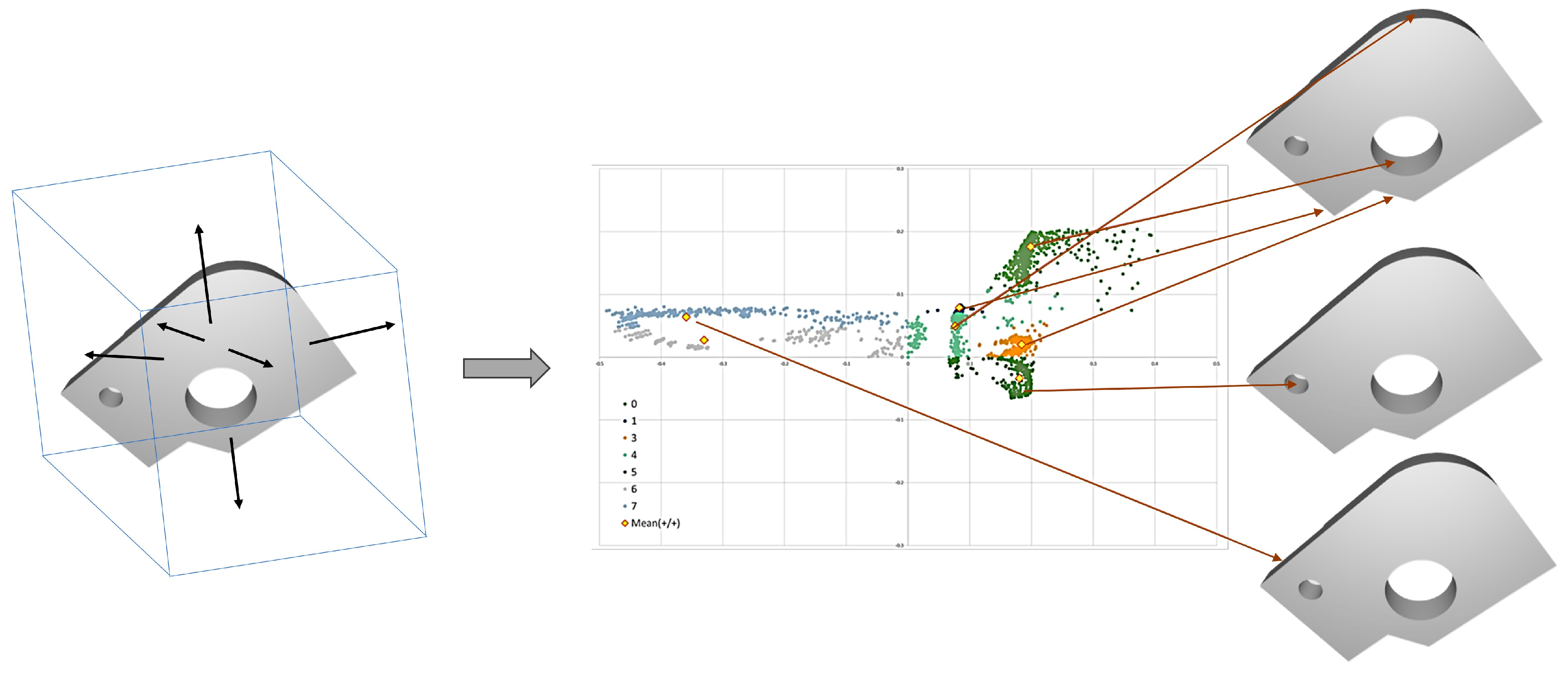
Figure 3 illustrates how the shape from
Figure 1 is mapped to the environment using cube mapping and the Equations (1) and (2). The (
u,
v) texture coordinates on the environment map corresponding to the direction of the surface normal vector
N are calculated.
One of the EM limitations is the potential for distortion, particularly when using techniques like sphere and cube mappings. In computer graphics, these distortions can become noticeable when the mapped environment has strong features or when the object’s shape does not align well with the mapping method. Additionally, EM is inherently an approximation technique. It simplifies the complex interactions of light, and as such, it cannot account for phenomena like multiple reflections or refractions. This means that while EM can create a convincing illusion of reflection, it does not replicate the true physics of light, which can be a drawback in scenarios where photorealism is required.
However, such distortion and approximation techniques are advantageous when performing classification in RE, and this is the reason EM is used in this paper. To create a mesh from 3D points and perform classification directly from this mesh, we must either use a template or the user's intuition as in previous researches, or go through many preprocessing processes. But, when EM is used, the properties of the primitive for classification are maintained while the properties are approximated, distorted, and mapped to the environment, making it insensitive to noise.
2.3. Learning through SL
To use the SL method, labels are required. In this paper, the basic shapes to be classified through RE are broadly categorized into: 1) plane, 2) cylinder, 3) torus, 4) sphere, 5) cone, 6) fillet, and 7) freeform shape. The shapes from 1 (plane) to 6 (fillet) are learned using the SL, while any other shape is considered a 7) freeform shape.
For SL, train data is generated by scanning objects corresponding to the plane through fillet (1~6) using a 3D scanner, and then generating the (u, v) coordinate clouds on the cube using the EM. Due to the limited number of real 3D datasets, the actual datasets of the plane through fillet (1~6) are scanned, then the normal vector N for each point of the datasets is randomly altered within the range of -2π ~ 2π to generate additional train data.
The next step involves generating a bounding box that encloses the created (u, v) coordinates. In traditional computer graphics, there are mainly three methods for creating bounding boxes: AABB (Axis-Aligned Bounding Box), OBB (Oriented Bounding Box), and k-dop (discrete orientation polytope). The bounding box more tightly encloses the object when using OBB and k-dop compared with the AABB. However, since the OBB and k-dop algorithms commonly used in computer graphics require heavy computational resources, this paper uses a modified OBB method, given that the cube map of the EM is similar to the AABB form.
First, the centroid of the clouds (
c1,
c2) is determined. Assuming it as an AABB, when the
u-axis is considered as the width and the
v-axis as the height, the lengths at both ends are taken as
umax and
vmax respectively, and the centroid of these lengths is set as (
c1,
c2).
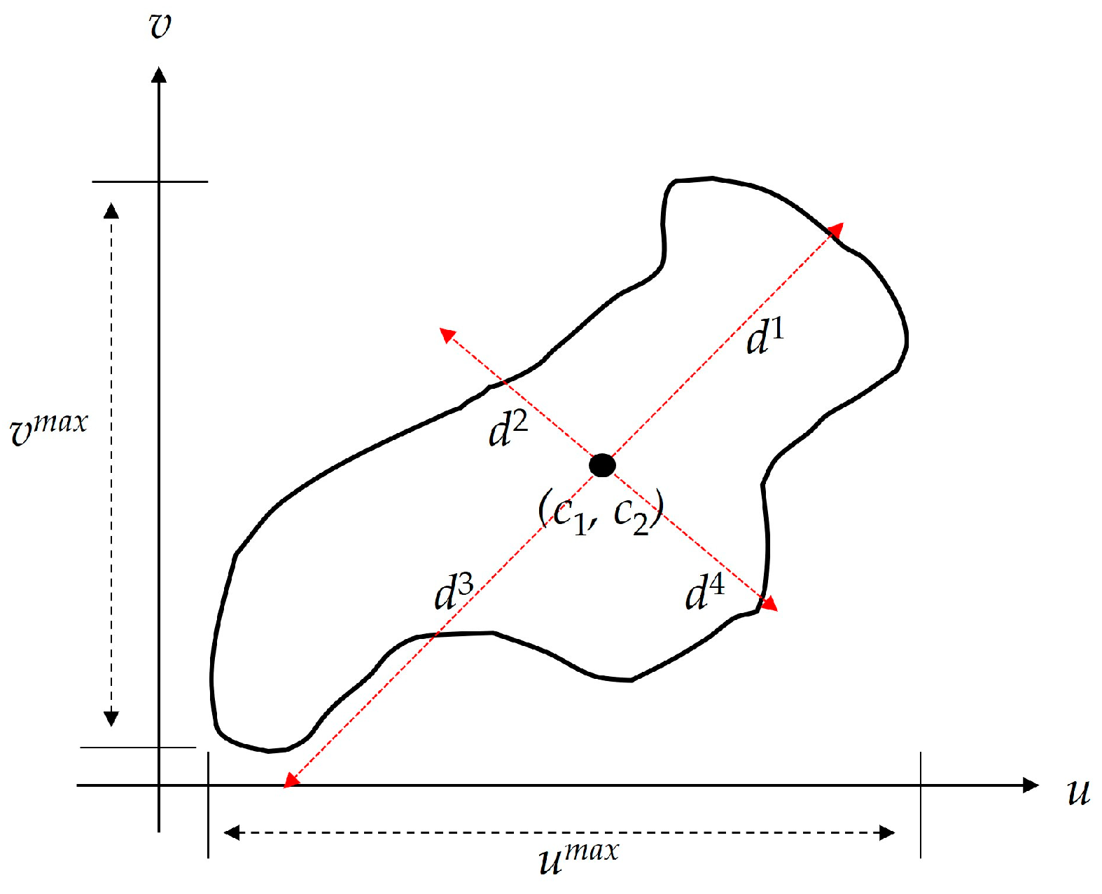
From this centroid, the maximum diagonal lengths (
d1,
d2,
d3, and
d4) are calculated.
Figure 4 shows an example of the six lengths (
umax,
vmax,
d1~
d4) used from cube on the EM.
These six calculated length data points are used as training data (input data), and the label corresponds to the six shapes (plane through fillet (1~6)) for training. Detailed hyperparameters for training are discussed in the next section 3.
After training, in the actual application phase, when arbitrary 3D point data is input, it is mapped onto the cube using the EM method described in section 2.2. After mapping, the six lengths (
umax,
vmax,
d1~
d4) are calculated from the (
c1,
c2), and the shape is classified into one of the six shapes. If the result falls below a user-defined threshold, it is classified as a freeform shape (7). The top side of
Figure 5 shows the training phase, while the bottom one depicts the actual application flowchart.
3. Experimental Results
To train using SL, 3D scanning was conducted on 20 actual objects for each of the six shapes (plane through fillet (1~6)). For training datasets, the 120 (= 20x6) scanned datasets were increased by randomly altering the normal vector
N within the range of -2π to 2π, as mentioned in
Section 2.3. I generate additional 10,000 datasets per the shape, so total I acquire the 60,120 datasets (that is, sum of 60,000 simulated data and 12 actual scan data). They were split into training, validation, and test datasets in a ratio of 8:1:1.
As shown in
Table 1, the hyper-parameters used were: an optimizer of Adam, initial learning rate of 0.0001, early stopping for the epoch, a batch size of 64, categorical cross-entropy as the loss function, and softmax as the activation function.
The experiment was conducted on Google COLABTM, achieving an accuracy of 0.9187 and an F1-score of 0.9812.
The experiment was conducted on a total of 20 newly scanned datasets.
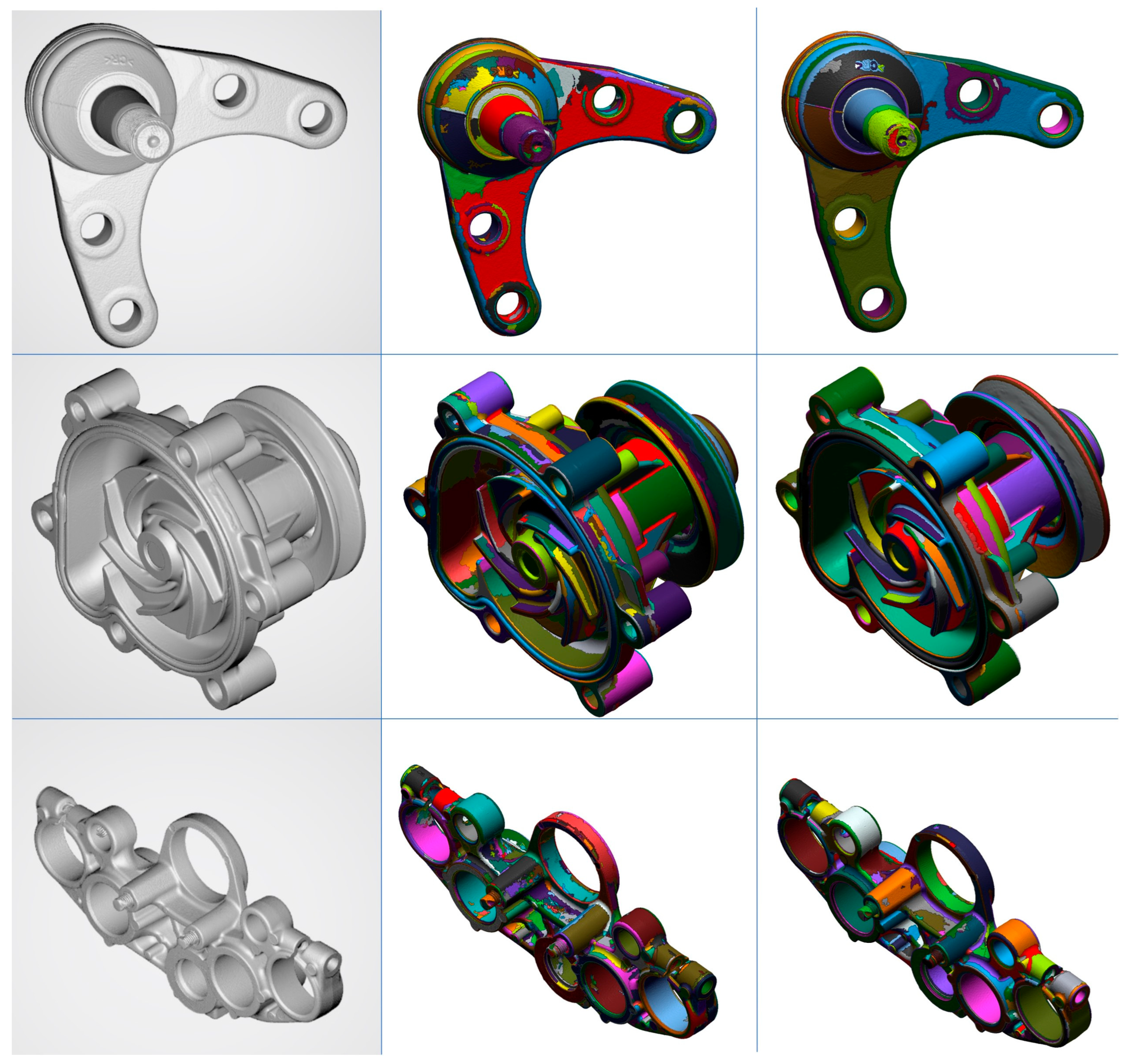
Figure 6 is a result capture image of three pieces of data (ball joint, water pump, and triple clamp datasets) out of total 20 experimental data. This data is publicly available on the internet under Creative Commons license v4 (copy and redistribute the material in any medium or format for any purpose, even commercially) [
24]. The middle side is the result of classification after completing the preprocessing process for comparison using conventional method [
16], and the right side is the result using the method proposed in this paper. Since there are few attempts similar to the method proposed in this paper, I compared it with the existing template-based method.
Table 2 shows the final vertex counts for the data in
Figure 6. After classification, the remeshing process was performed according to the identified primitives, resulting in a reduced number of vertices. Similar reductions in vertex counts, around 55%, were observed across the remaining 18 datasets, albeit with slight variations. This indicates a potential reduction in computational load in subsequent steps.


